

A Comparative Study and Optimization of Camera-Based BEV Segmentation for Real-Time Autonomous Driving

Abstract
1. Introduction
- Selection of the BEV image encoder, view transformation, and BEV decoder models: Based on the evaluation of mIoU accuracy, model size, and latency performance, the optimal image encoder, view transformation, and BEV decoder models were determined.
- Determination of the BEV input image size and data augmentation: The optimal image size was selected through a performance comparison across resolutions of , , and . Additionally, suitable data augmentation strategies were identified.
- Lightweight model optimization: Quantization techniques were applied to the model, and its accuracy and latency were measured to implement a lightweight optimization strategy for real-time autonomous driving embedded systems. Furthermore, the BEV segmentation performance was analyzed on-device, specifically deploying the model on the NVIDIA AGX Orin platform to assess its real-world applicability and to derive corresponding deployment strategies.
2. Related Work
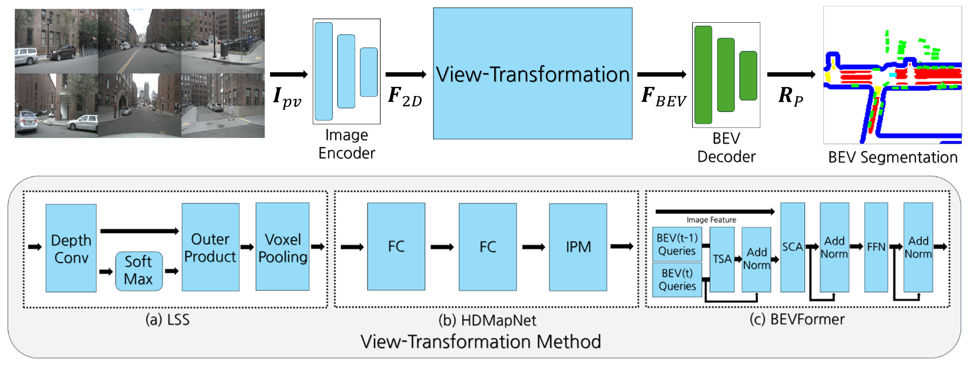
3. System Model
3.1. Image Encoder
3.2. View Transformation
3.2.1. Depth-Based Method
3.2.2. MLP-Based Method
3.2.3. Transformer-Based Method
3.3. BEV Decoder
4. Performance Enhancement Strategy
4.1. Evaluation Metrics
4.2. BEV Enhancement Methodology
4.2.1. Model Determination
4.2.2. Model Enhancement
4.2.3. Model Compression
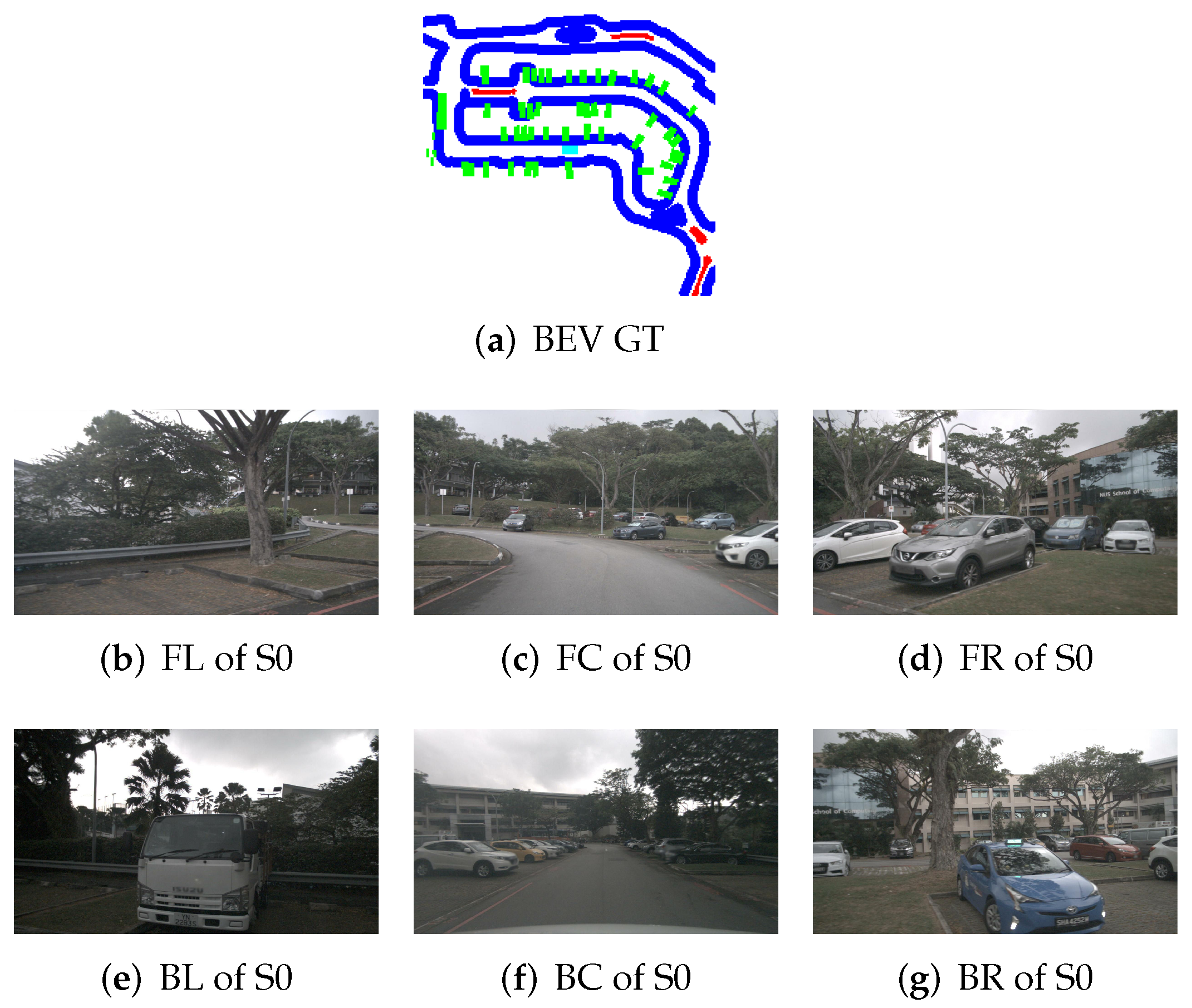
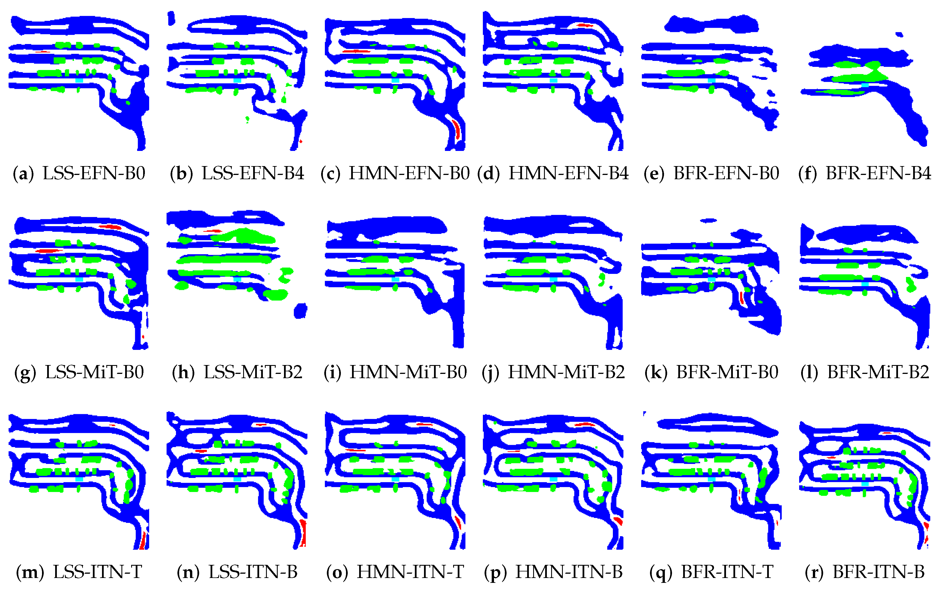
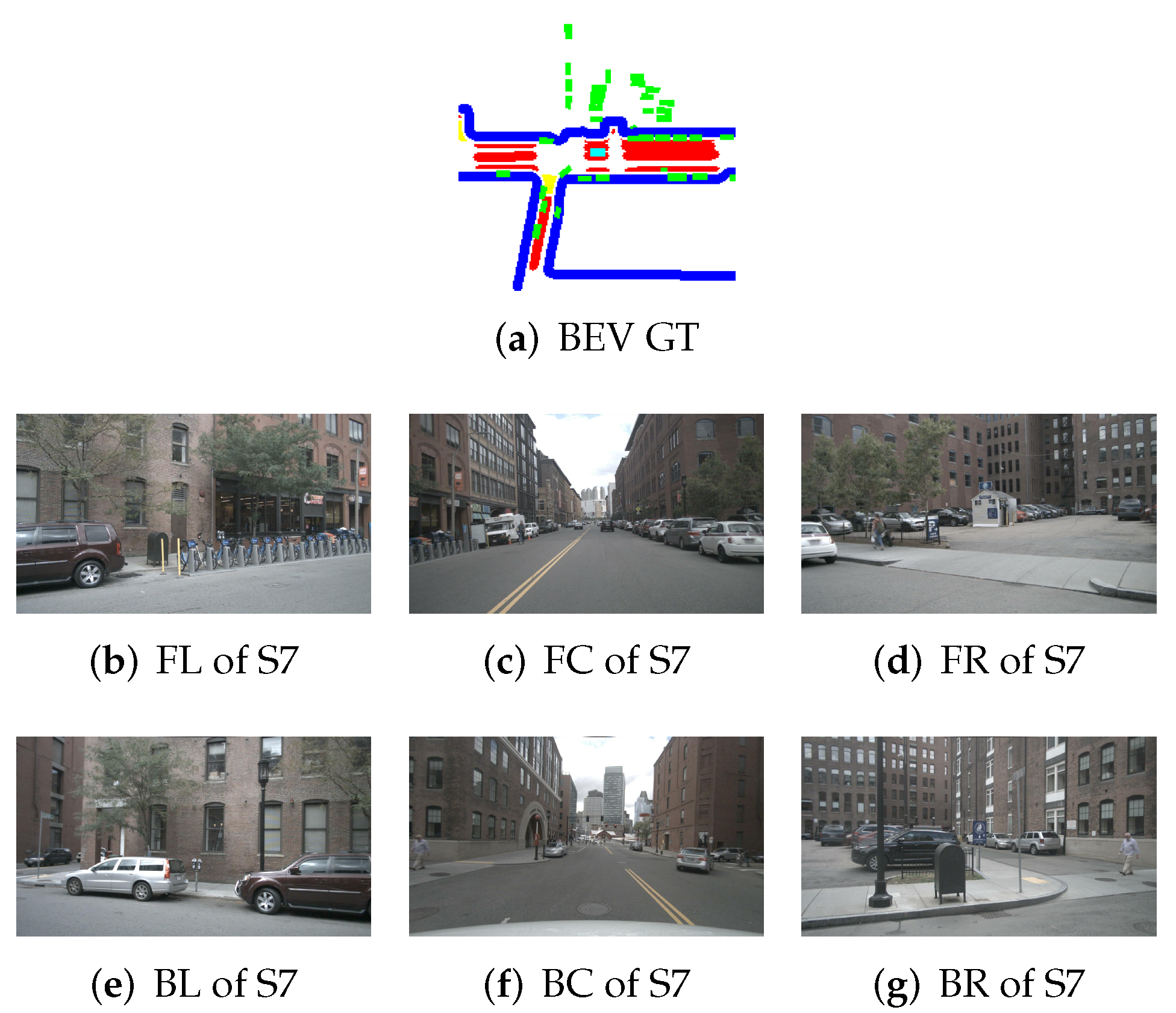
5. Simulation Result
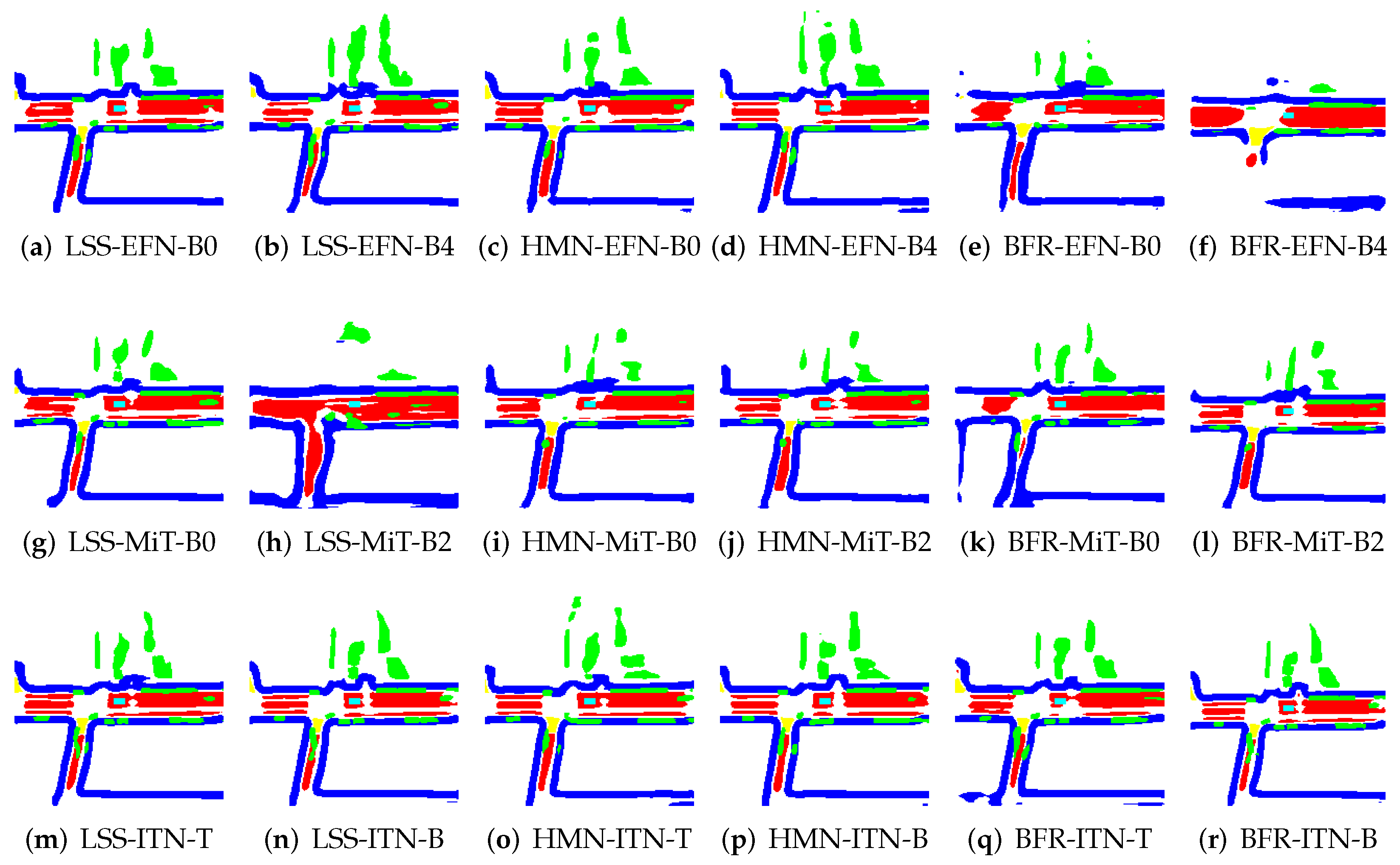
5.1. Model Determination
5.2. Model Enhancement
5.3. Model Compression
6. Discussion
6.1. Failure Cases and Limitations: Heavy Traffic
6.2. High-Speed Driving
6.3. Inference Acceleration
6.4. Sensor Innovation
7. Conclusions
Author Contributions
Funding
Data Availability Statement
Conflicts of Interest
References
- Yurtserver, E.; Lambert, J.; Carballo, A.; Takeda, K. A Survey of Autonomous Driving: Common Practices and Emerging Technologies. IEEE Access 2020, 8, 58443–58469. [Google Scholar] [CrossRef]
- Zhao, J.; Zhao, W.; Deng, B.; Wang, Z.; Zhang, F.; Zheng, W.; Cao, W.; Nan, J.; Lian, Y.; Burke, A.F. Autonomous driving system: A comprehensive survey. Expert Syst. Appl. 2024, 242, 122836. [Google Scholar] [CrossRef]
- Tampuu, A.; Semikin, M.; Muhammad, N.; Fishman, D.; Matiisen, T. A Survey of End-to-End Driving: Architectures and Training Methods. IEEE Trans. Neural Netw. Learn. Syst. 2022, 33, 1364–1384. [Google Scholar] [CrossRef] [PubMed]
- Yang, Z.; Li, X.J.H.; Yan, J. LLM4Drive: A Survey of Large Language Models for Autonomous Driving. arXiv 2023, arXiv:2311.01043. [Google Scholar] [CrossRef]
- Xu, H.; Chen, J.; Meng, S.; Wang, Y.; Chau, L.-P. A Survey on Occupancy Perception for Autonomous Driving: The Information Fusion Perspective. arXiv 2024, arXiv:2405.05173. [Google Scholar] [CrossRef]
- Roddick, T.; Kendall, A.; Cipolla, R. Orthographic Feature Transform for Monocular 3D Object Detection. arXiv 2018, arXiv:1811.08188. [Google Scholar] [CrossRef]
- Philion, J.; Fidler, S. Lift, Splat, Shoot: Encoding Images from Arbitrary Camera Rigs by Implicitly Unprojecting to 3D. ECCV 2020 LNIP 2020, 12359, 194–210. [Google Scholar]
- Wang, Y.; Chao, W.-L.; Garg, D.; Hariharan, B.; Campbell, M.; Weinberger, K.Q. Pseudo-LiDAR from Visual Depth Estimation: Bridging the Gap in 3D Object Detection for Autonomous Driving. In Proceedings of the 2019 IEEE/CVF Conference on Computer Vision and Pattern Recognition (CVPR), Long Beach, CA, USA, 15–20 June 2019; pp. 8445–8453. [Google Scholar] [CrossRef]
- Huang, J.; Huang, G.; Zhu, Z.; Ye, Y.; Du, D. BEVDet: High-performance Multi-camera 3D Object Detection in Bird-Eye-View. arXiv 2022, arXiv:2112.11790. [Google Scholar] [CrossRef]
- Harley, A.W.; Fang, Z.; Li, J.; Ambrus, R.; Fragkiadaki, K. Simple-BEV: What Really Matters for Multi-Sensor BEV Perception? In Proceedings of the IEEE International Conference on Robotics and Automation (ICRA), London, UK, 29 May–2 June 2023. [Google Scholar]
- Lang, A.H.; Vora, S.; Caesar, H.; Zhou, L.; Yang, J.; Beijbom, O. PointPillars: Fast Encoders for Object Detection from Point Clouds. In Proceedings of the 2019 IEEE/CVF Conference on Computer Vision and Pattern Recognition (CVPR), Long Beach, CA, USA, 15–20 June 2019; pp. 12689–12697. [Google Scholar] [CrossRef]
- Ma, Y.; Wang, T.; Bai, X.; Yang, H.; Hou, Y.; Wang, Y.; Qiao, Y.; Yang, R.; Manocha, D.; Zhu, X. Vision-Centric BEV Perception: A Survey. arXiv 2022, arXiv:2208.02797. [Google Scholar] [CrossRef]
- Pan, B.; Sun, J.; Leung, H.Y.T.; Andonian, A.; Zhou, B. Cross-view Semantic Segmentation for Sensing Surroundings. IEEE Robot. Autom. Lett. 2020, 5, 4867–4873. [Google Scholar] [CrossRef]
- Li, Q.; Wang, Y.; Wang, Y.; Zhao, H. HDMapNet: An online HD map Construction and Evaluation Framework. In Proceedings of the 2022 International Conference on Robotics and Automation (ICRA), Philadelphia, PA, USA, 23–27 May 2022. [Google Scholar] [CrossRef]
- Lu, C.; ven de Molengraft, M.J.G.; Dubblman, G. Monocular Semantic Occupancy Grid Mapping with Convolutional Variational Encoder-Decoder Networks. IEEE Robot. Auto. Lett. 2019, 4, 2. [Google Scholar] [CrossRef]
- Roddick, T.; Cipolla, R. Predicting Semantic Map Representations from Images using Pyramid Occupancy Networks. In Proceedings of the 2020 IEEE/CVF Conference on Computer Vision and Pattern Recognition (CVPR), Seattle, WA, USA, 13–19 June 2020; pp. 11138–11147. [Google Scholar] [CrossRef]
- Jiang, Y.; Zhang, L.; Miao, Z.; Zhu, X.; Gao, J.; Hu, W.; Jiang, Y.-G. PolarFormer: Multi-Camera 3D Object Detection with Polar Transformer. AAAI Conf. 2023, 37, 1042–1050. [Google Scholar] [CrossRef]
- Li, Z.; Wang, W.; Li, H.; Xie, E.; Sima, C.; Lu, T.; Yu, Q.; Dai, J. BEVFormer: Learning Bird’s-Eye-View Representation from Multi-Camera Images via Spatiotemporal Transformers. In Proceedings of the 2022 European Conference on Computer Vision, Tel Aviv, Israel, 23–27 October 2022; Volume 13669, pp. 1–18. [Google Scholar] [CrossRef]
- Wang, Y.; Guizilini, V.; Zhang, T.; Wang, Y.; Zhao, H.; Solomon, J. DETR3D: 3D Object Detection from Multi-view Images via 3D-to-2D Queries. In Proceedings of the 5th Conference on Robot Learning, London, UK, 8–11 November 2021; Volume 164, pp. 180–191. [Google Scholar] [CrossRef]
- Tan, M.; Le, Q.V. EfficientNet: Rethinking Model Scaling for Convolutional Neural Networks. PMLR 2019, 97, 6105–6114. [Google Scholar]
- Xie, E.; Wang, W.; Yu, Z.; Anandkumar, A.; Alvarez, J.M.; Luo, P. SegFormer: Simple and Efficient Design for Semantic Segmentation with Transformers. Adv. NeurIPS 2021, 34, 12077–12090. [Google Scholar] [CrossRef]
- Wang, W.; Dai, J.; Chen, Z.; Huang, Z.; Li, Z.; Zhu, X.; Hu, X.; Lu, T.; Li, H.; Wang, X.; et al. InternImage: Exploring Large-Scale Vision Foundation Models with Deformable Convolutions. In Proceedings of the IEEE/CVF Conference on Computer Vision and Pattern Recognition (CVPR), Vancouver, BC, Canada, 17–24 June 2023; pp. 14408–14419. [Google Scholar]
- Lee, H.; Lee, N.; Lee, S. A Method of Deep Learning Model Optimization for Image Classification on Edge Device. Sensors 2022, 22, 7344. [Google Scholar] [CrossRef]
- Caesar, H.; Bankiti, V.; Lang, A.H.; Vora, S.; Liong, V.E.; Xu, Q.; Krishnan, A.; Pan, Y.; Baldan, G.; Beijbom, O. nuScenes: A multimodal dataset for autonomous driving. In Proceedings of the IEEE/CVF Conference on Computer Vision and Pattern Recognition (CVPR), Seattle, WA, USA, 13–19 June 2020; pp. 11618–11628. [Google Scholar]
- Available online: https://www.nvidia.com/en-us/autonomous-machines/embedded-systems/jetson-orin/ (accessed on 27 March 2025).
- Dosovitskiy, A.; Ros, G.; Codevilla, F.; Lopez, A.; Koltun, V. CARLA: An Open Urban Driving Simulator. In Proceedings of the 1st Annual Conference on Robot Learning, Mountain View, CA, USA, 11–15 November 2017; pp. 1–16. [Google Scholar]
- Zhang, J.; Zhang, Y.; Qi, Y.; Fu, Z.; Liu1, Q.; Wang, Y. GeoBEV: Learning Geometric BEV Representation for Multi-view 3D Object Detection. arXiv 2024, arXiv:2409.01816v2. [Google Scholar]
- Available online: https://en.wikipedia.org/wiki/Motion_blur_(media) (accessed on 27 March 2025).
- Available online: https://en.wikipedia.org/wiki/Rolling_shutter (accessed on 27 March 2025).
- Huang, B.; Li, Y.; Xie, E.; Liang, F.; Wang, L.; Shen, M.; Liu, F.; Wang, T.; Luo, P.; Shao, J. Fast-BEV: Towards Real-time On-vehicle Bird’s-Eye View Perception. arXiv 2023, arXiv:2301.07870. [Google Scholar]
- Gallego, G.; Delbruck, T.; Orchard, G.; Bartolozzi, C.; Taba, B.; Censi, A.; Leutenegger, S.; Davison, A.; Conradt, J.; Daniilidis, K.; et al. Event-based Vision: A Survey. IEEE Trans. Pattern Anal. Mach. Intell. 2020, 44, 154–180. [Google Scholar]
- Available online: https://www.nvidia.com/en-us/geforce/graphics-cards/50-series/ (accessed on 27 March 2025).
- Zhong, J.; Liu, Z.; Chen, X. Transformer-based models and hardware acceleration analysis in autonomous driving: A survey. arXiv 2023, arXiv:2304.10891. [Google Scholar]
- Zhu, M.; Gong, Y.; Tian, C.; Zhu, Z. A Systematic Survey of Transformer-Based 3D Object Detection for Autonomous Driving: Methods, Challenges and Trends. Drones 2024, 8, 412. [Google Scholar] [CrossRef]
- Malcolm, K.; Casco-Rodriguez, J. A Comprehensive Review of Spiking Neural Networks: Interpretation, Optimization, Efficiency, and Best Practices. arXiv 2023, arXiv:2303.10780. [Google Scholar]


| Quantization Model | Acc (%) | Size (KB) | Lat (ms) |
|---|---|---|---|
| NQ | 80.7 | 94,052 | 177 |
| BLQ | 80.3 | 24,161 | 2348 |
| FIQ | 80.4 | 24,269 | 2078 |
| F16 | 80.6 | 47,072 | 152 |
| QAT | 80.5 | 24,281 | 2069 |
| Model | LSS (224 × 480) | |||||
| EFN-B0 | EFN-B4 | MiT-B0 | MiT-B2 | ITN-T | ITN-B | |
| mIoU | 46.4 | 47.7 | 44.8 | 46.2 | 51.3 | 52.2 |
| Latency | 21.9 | 30.5 | 19.7 | 25.8 | 30.6 | 37.7 |
| Size | 59.4 | 116.1 | 51.6 | 138.5 | 159.2 | 427.0 |
| Lane | 53.2 | 53.9 | 51.8 | 53.1 | 58.8 | 59.7 |
| Crosswalk | 42.3 | 44.1 | 39.7 | 40.7 | 51.5 | 52.1 |
| Bound | 57.2 | 58.6 | 55.6 | 56.8 | 63.0 | 63.9 |
| Car | 32.9 | 34.3 | 32.2 | 34.3 | 37.9 | 39.2 |
| Model | HMN (224 × 480) | |||||
| EFN-B0 | EFN-B4 | MiT-B0 | MiT-B2 | ITN-T | ITN-B | |
| mIoU | 42.3 | 43.7 | 39.9 | 38.7 | 47.1 | 48.6 |
| Latency | 22.4 | 30.9 | 20.0 | 25.9 | 30.4 | 33.6 |
| Size | 117.6 | 171.6 | 110.0 | 190.6 | 212.3 | 471.2 |
| Lane | 50.4 | 51.2 | 47.6 | 45.9 | 54.4 | 55.4 |
| Crosswalk | 37.3 | 39.4 | 35.6 | 33.2 | 44.0 | 46.0 |
| Bound | 53.5 | 55.0 | 50.7 | 48.9 | 58.1 | 59.8 |
| Car | 28.0 | 29.4 | 25.9 | 26.9 | 31.9 | 33.3 |
| Model | BFR (224 × 480) | |||||
| EFN-B0 | EFN-B4 | MiT-B0 | MiT-B2 | ITN-T | ITN-B | |
| mIoU | 35.3 | 40.1 | 42.3 | 39.3 | 48.0 | 50.2 |
| Latency | 39.1 | 49.1 | 34.0 | 39.2 | 47.5 | 53.5 |
| Size | 66.5 | 76.4 | 76.12 | 157.5 | 179.15 | 439.3 |
| Lane | 41.5 | 46.3 | 49.1 | 46.7 | 54.6 | 56.7 |
| Crosswalk | 29.9 | 34.5 | 37.6 | 31.5 | 44.6 | 47.2 |
| Bound | 45.2 | 50.3 | 53.0 | 51.0 | 58.4 | 60.8 |
| Car | 24.9 | 29.5 | 29.8 | 28.4 | 34.5 | 36.2 |
| Model | LSS (448 × 800) | |||||
| EFN-B0 | EFN-B4 | MiT-B0 | MiT-B2 | ITN-T | ITN-B | |
| mIoU | 49.1 | 48.3 | 47.7 | 48.3 | 53.1 | 54.9 |
| Latency | 30.1 | 50.1 | 28.8 | 50.0 | 51.7 | 95.5 |
| Size | 59.7 | 116.4 | 51.9 | 138.8 | 159.5 | 427.3 |
| Lane | 54.6 | 55.3 | 54.5 | 55.8 | 58.8 | 60.5 |
| Crosswalk | 46.1 | 45.7 | 43.2 | 45.0 | 51.0 | 53.6 |
| Bound | 59.6 | 60.0 | 58.1 | 59.6 | 62.8 | 64.5 |
| Car | 36.1 | 38.3 | 35.0 | 33.1 | 40.0 | 41.2 |
| Model | HMN (448 × 800) | |||||
| EFN-B0 | EFN-B4 | MiT-B0 | MiT-B2 | ITN-T | ITN-B | |
| mIoU | 44.1 | 43.2 | 42.5 | 43.2 | 45.8 | 50.7 |
| Latency | 25.5 | 39.1 | 23.1 | 38.9 | 40.2 | 83.7 |
| Size | 153.5 | 207.5 | 145.7 | 226.5 | 248.2 | 507.1 |
| Lane | 51.4 | 50.2 | 49.7 | 49.4 | 52.2 | 57.3 |
| Crosswalk | 40.2 | 38.2 | 37.3 | 38.6 | 42.1 | 48.1 |
| Bound | 54.8 | 53.9 | 29.6 | 54.2 | 56.1 | 60.8 |
| Car | 30.2 | 30.5 | 42.5 | 30.8 | 33.0 | 36.6 |
| Model | BFR (448 × 800) | |||||
| EFN-B0 | EFN-B4 | MiT-B0 | MiT-B2 | ITN-T | ITN-B | |
| mIoU | 38.9 | 26.7 | 44.1 | 44.8 | 50.8 | 53.9 |
| Latency | 43.3 | 60.4 | 44.3 | 65.7 | 64.5 | 106.8 |
| Size | 66.5 | 76.4 | 76.12 | 157.5 | 179.14 | 439.3 |
| Lane | 44.3 | 31.2 | 50.7 | 51.7 | 56.8 | 59.8 |
| Crosswalk | 34.1 | 18.5 | 39.6 | 39.9 | 47.7 | 51.9 |
| Bound | 49.1 | 35.9 | 54.2 | 55.5 | 60.5 | 63.7 |
| Car | 28.3 | 21.2 | 31.9 | 32.0 | 38.2 | 40.1 |
| Model | EFN-B0 | MiT-B0 | ITN-T |
| mIoU | 51.3 | 50.7 | 51.9 |
| Latency | 30.6 | 28.5 | 34.2 |
| Size | 159.2 | 151.8 | 254.0 |
| Model | EFN-B4 | MiT-B4 | ITN-B |
| mIoU | 52.0 | 51.1 | 52.7 |
| Latency | 32.1 | 33.5 | 41.2 |
| Size | 213.9 | 232.3 | 512.9 |
| Encoder Model | Top-1 Acc (%) | Params (M) |
|---|---|---|
| EFN-B0 | 77.1 | 5.3 |
| EFN-B4 | 82.9 | 19.0 |
| MiT-B0 | 70.5 | 3.7 |
| MiT-B2 | 81.6 | 25.4 |
| ITN-T | 83.5 | 30.0 |
| ITN-B | 84.9 | 97.0 |
| Model | LSS | HMN | BFR |
|---|---|---|---|
| mIoU | 52.7 | 48.1 | 52.8 |
| Latency | 197.2 | 68.2 | 209.5 |
| Size | 160.3 | 312.4 | 179.1 |
| 224 × 480 | HMN | LSS | BFR |
| mIoU | 62.1 | 64.0 | 65.5 |
| DAS | 89.2 | 89.1 | 89.1 |
| Lane | 44.1 | 47.1 | 49.1 |
| Vehicle | 53.2 | 56.0 | 58.4 |
| 448 × 800 | HMN | LSS | BFR |
| mIoU | 62.8 | 65.5 | 67.5 |
| DAS | 89.4 | 91.0 | 91.7 |
| Lane | 45.1 | 48.1 | 51.7 |
| Vehicle | 54.0 | 57.4 | 59.1 |
| 672 × 1200 | HMN | LSS | BFR |
| mIoU | 64.3 | 65.6 | 67.9 |
| DAS | 90.5 | 91.7 | 91.1 |
| Lane | 46.0 | 48.1 | 52.0 |
| Vehicle | 56.4 | 57.1 | 60.7 |
| Model | LSS DataAug | HMN DataAug | BFR DataAug |
|---|---|---|---|
| mIoU | 51.6 | 43.2 | 49.3 |
| Latency | 51.3 | 40.6 | 64.2 |
| Size | 160.3 | 312.4 | 179.1 |
| Model | Quantized LSS (224 × 480) | |||||
| EFN-B0 | EFN-B4 | MiT-B0 | MiT-B2 | ITN-T | ITN-B | |
| mIoU | 44.7 | 45.9 | 43.1 | 44.2 | 49.0 | 49.9 |
| Latency | 21.7 | 30.2 | 19.4 | 25.6 | 30.2 | 37.4 |
| Size | 29.7 | 58.0 | 25.8 | 69.2 | 79.6 | 213.5 |
| Model | Quantized HDMapNet (224 × 480) | |||||
| EFN-B0 | EFN-B4 | MiT-B0 | MiT-B2 | ITN-T | ITN-B | |
| mIoU | 42.3 | 43.7 | 39.8 | 38.7 | 47.1 | 48.6 |
| Latency | 22.2 | 30.7 | 19.9 | 25.7 | 30.2 | 33.4 |
| Size | 58.8 | 85.8 | 55.0 | 95.3 | 106.2 | 235.6 |
| Model | Quantized BEVFormer (224 × 480) | |||||
| EFN-B0 | EFN-B4 | MiT-B0 | MiT-B2 | ITN-T | ITN-B | |
| mIoU | 33.8 | 38.6 | 40.8 | 37.8 | 46.5 | 48.7 |
| Latency | 39.0 | 48.9 | 33.9 | 39.0 | 47.3 | 53.3 |
| Size | 33.2 | 38.2 | 38.1 | 78.8 | 89.6 | 219.6 |
| Model | Quantized LSS (448 × 800) | |||||
| EFN-B0 | EFN-B4 | MiT-B0 | MiT-B2 | ITN-T | ITN-B | |
| mIoU | 47.1 | 46.1 | 45.8 | 46.4 | 51.3 | 53.0 |
| Latency | 29.8 | 49.8 | 28.6 | 49.8 | 51.9 | 95.3 |
| Size | 29.8 | 58.2 | 26.0 | 69.4 | 79.8 | 213.6 |
| Model | Quantized HDMapNet (448 × 800) | |||||
| EFN-B0 | EFN-B4 | MiT-B0 | MiT-B2 | ITN-T | ITN-B | |
| mIoU | 44.1 | 43.2 | 42.5 | 43.1 | 45.8 | 50.7 |
| Latency | 25.7 | 38.9 | 22.8 | 38.8 | 40.1 | 83.6 |
| Size | 76.8 | 103.8 | 72.8 | 113.2 | 124.1 | 253.6 |
| Model | Quantized BEVFormer (448 × 800) | |||||
| EFN-B0 | EFN-B4 | MiT-B0 | MiT-B2 | ITN-T | ITN-B | |
| mIoU | 37.4 | 25.2 | 42.5 | 43.3 | 49.3 | 52.4 |
| Latency | 43.2 | 60.0 | 44.1 | 65.5 | 64.3 | 106.7 |
| Size | 33.2 | 38.2 | 38.1 | 78.8 | 89.6 | 219.6 |
| Model | Quantized LSS (224 × 480) | |||||
| EFN-B0 | EFN-B4 | MiT-B0 | MiT-B2 | ITN-T | ITN-B | |
| mIoU | 44.7 | 45.9 | 43.1 | 44.2 | 49.0 | 49.9 |
| Latency (30 W) | 182.8 | 321.1 | 170.5 | 289.7 | 392.6 | 634.2 |
| Latency (50 W) | 136.4 | 204.9 | 124.8 | 177.9 | 216.9 | 319.7 |
| Model | Quantized HDMapNet (224 × 480) | |||||
| EFN-B0 | EFN-B4 | MiT-B0 | MiT-B2 | ITN-T | ITN-B | |
| mIoU | 42.3 | 43.7 | 39.8 | 38.7 | 47.1 | 48.6 |
| Latency (30 W) | 141.9 | 283.1 | 136.6 | 249.5 | 353.5 | 587.1 |
| Latency (50 W) | 124.4 | 157.8 | 112.8 | 132.7 | 153.1 | 255.4 |
| Model | Quantized BEVFormer (224 × 480) | |||||
| EFN-B0 | EFN-B4 | MiT-B0 | MiT-B2 | ITN-T | ITN-B | |
| mIoU | 33.8 | 38.6 | 40.8 | 37.8 | 46.5 | 48.7 |
| Latency (30 W) | 820.0 | 946.8 | 825.9 | 917.9 | 964.0 | 1283.6 |
| Latency (50 W) | 393.3 | 399.7 | 299.3 | 413.9 | 432.8 | 600.9 |
| Model | Quantized LSS (448 × 800) | |||||
| EFN-B0 | EFN-B4 | MiT-B0 | MiT-B2 | ITN-T | ITN-B | |
| mIoU | 47.1 | 46.1 | 45.8 | 46.4 | 51.3 | 53.0 |
| Latency (30 W) | 448.1 | 929.7 | 494.6 | 886.7 | 1167.3 | 1931.4 |
| Latency (50 W) | 324.1 | 537.4 | 311.6 | 489.8 | 582.0 | 901.1 |
| Model | Quantized HDMapNet (448 × 800) | |||||
| EFN-B0 | EFN-B4 | MiT-B0 | MiT-B2 | ITN-T | ITN-B | |
| mIoU | 44.1 | 43.2 | 42.5 | 43.1 | 45.8 | 50.7 |
| Latency (30 W) | 319.4 | 756.8 | 329.8 | 706.3 | 997.2 | 1743.4 |
| Latency (50 W) | 211.5 | 404.9 | 200.2 | 346.9 | 454.4 | 732.4 |
| Model | Quantized BEVFormer (448 × 800) | |||||
| EFN-B0 | EFN-B4 | MiT-B0 | MiT-B2 | ITN-T | ITN-B | |
| mIoU | 37.4 | 25.2 | 42.5 | 43.3 | 49.3 | 52.4 |
| Latency (30 W) | 980.7 | 1128.1 | 930.6 | 1353.4 | 1669.9 | 2311.7 |
| Latency (50 W) | 457.0 | 618.2 | 464.2 | 615.26 | 714.4 | 1059.4 |
Disclaimer/Publisher’s Note: The statements, opinions and data contained in all publications are solely those of the individual author(s) and contributor(s) and not of MDPI and/or the editor(s). MDPI and/or the editor(s) disclaim responsibility for any injury to people or property resulting from any ideas, methods, instructions or products referred to in the content. |
© 2025 by the authors. Licensee MDPI, Basel, Switzerland. This article is an open access article distributed under the terms and conditions of the Creative Commons Attribution (CC BY) license (https://creativecommons.org/licenses/by/4.0/).
Share and Cite
Jun, W.; Lee, S. A Comparative Study and Optimization of Camera-Based BEV Segmentation for Real-Time Autonomous Driving. Sensors 2025, 25, 2300. https://doi.org/10.3390/s25072300
Jun W, Lee S. A Comparative Study and Optimization of Camera-Based BEV Segmentation for Real-Time Autonomous Driving. Sensors. 2025; 25(7):2300. https://doi.org/10.3390/s25072300
Chicago/Turabian StyleJun, Woomin, and Sungjin Lee. 2025. "A Comparative Study and Optimization of Camera-Based BEV Segmentation for Real-Time Autonomous Driving" Sensors 25, no. 7: 2300. https://doi.org/10.3390/s25072300
APA StyleJun, W., & Lee, S. (2025). A Comparative Study and Optimization of Camera-Based BEV Segmentation for Real-Time Autonomous Driving. Sensors, 25(7), 2300. https://doi.org/10.3390/s25072300