
Evaluation of Low-Cost Multi-Spectral Sensors for Measuring Chlorophyll Levels Across Diverse Leaf Types


Abstract
1. Introduction
2. Materials and Methods
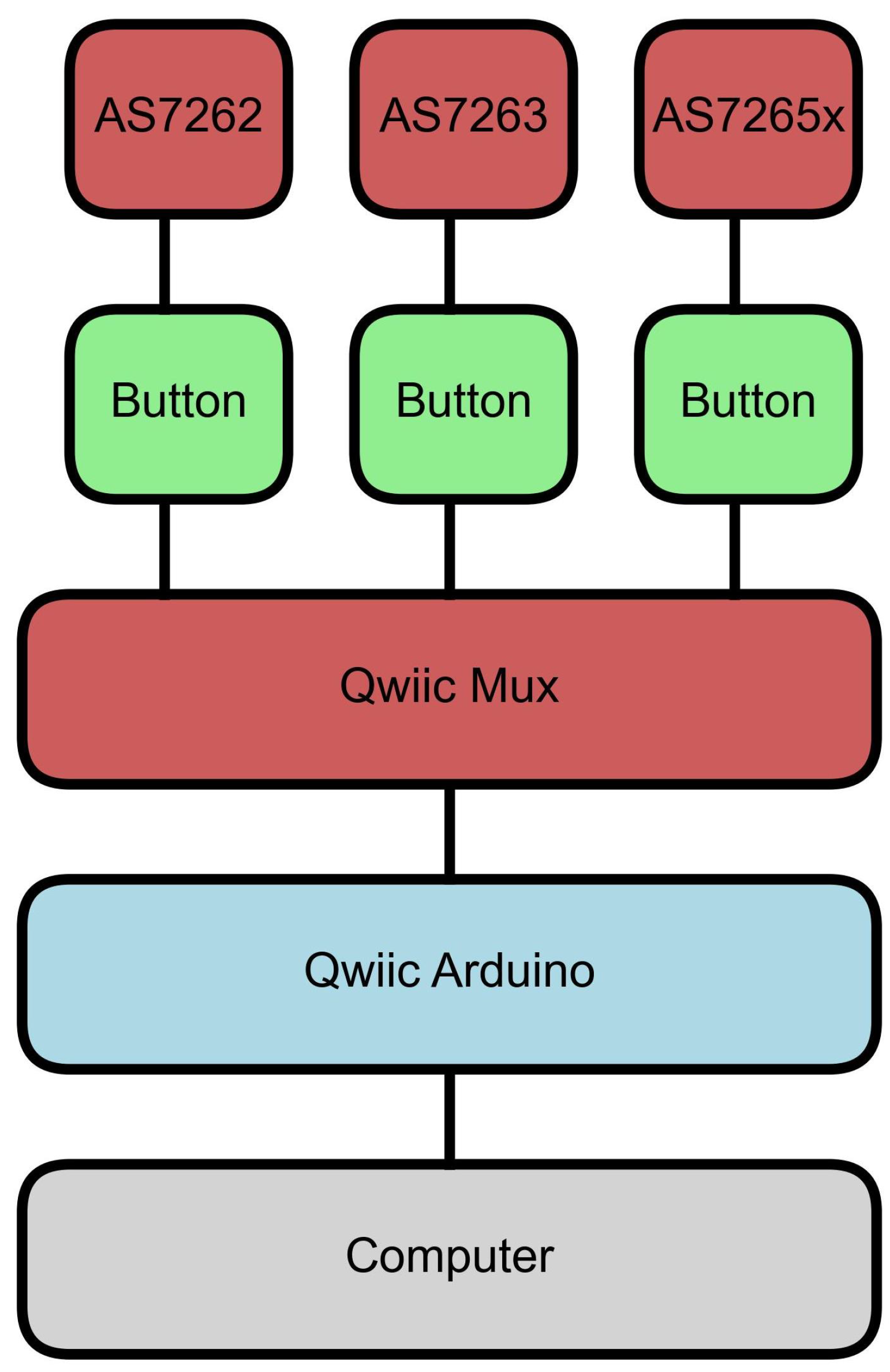
2.1. Device Design and Characterization
2.2. Device Firmware and Software
2.3. Leaf Selection and Spectra
2.4. Leaf Chlorophyll Measurements
2.5. Data Processing and Statistical Methods
3. Results
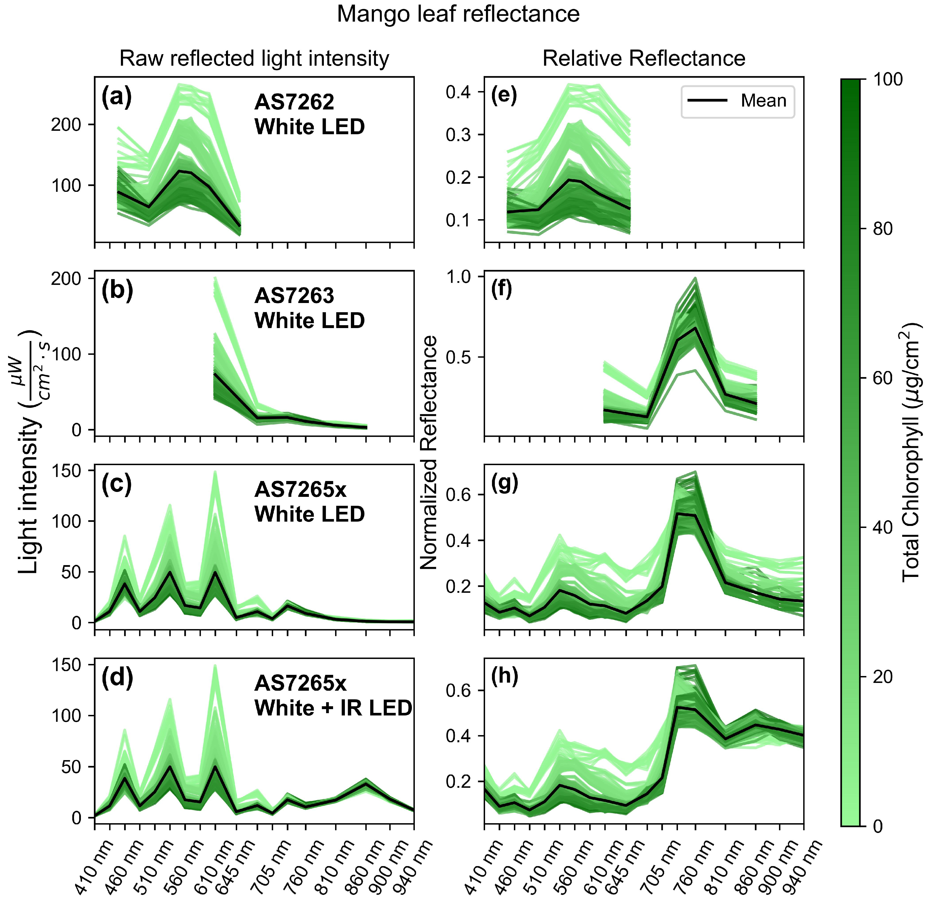
3.1. Leaf Spectra
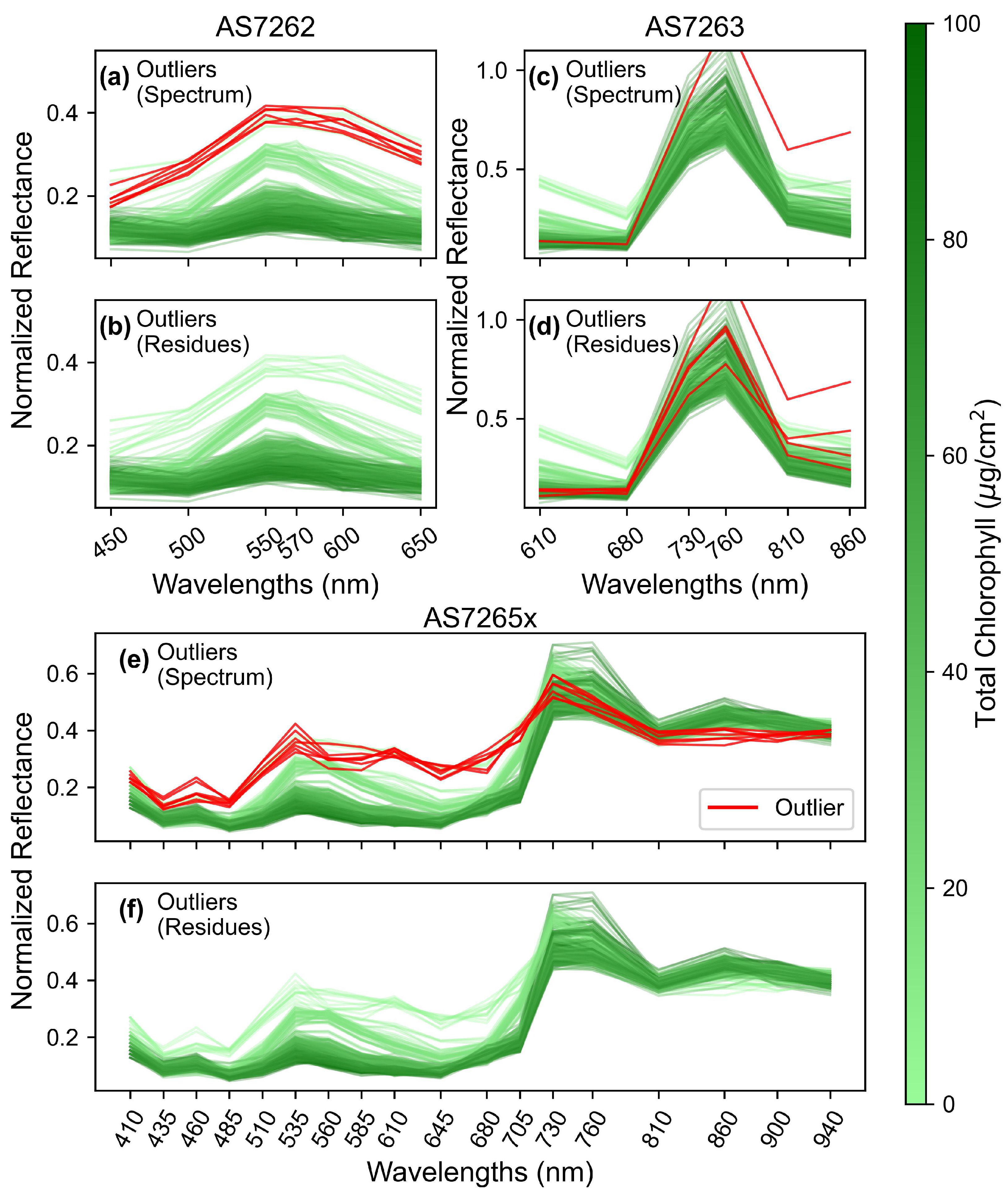
3.2. Outlier Detection
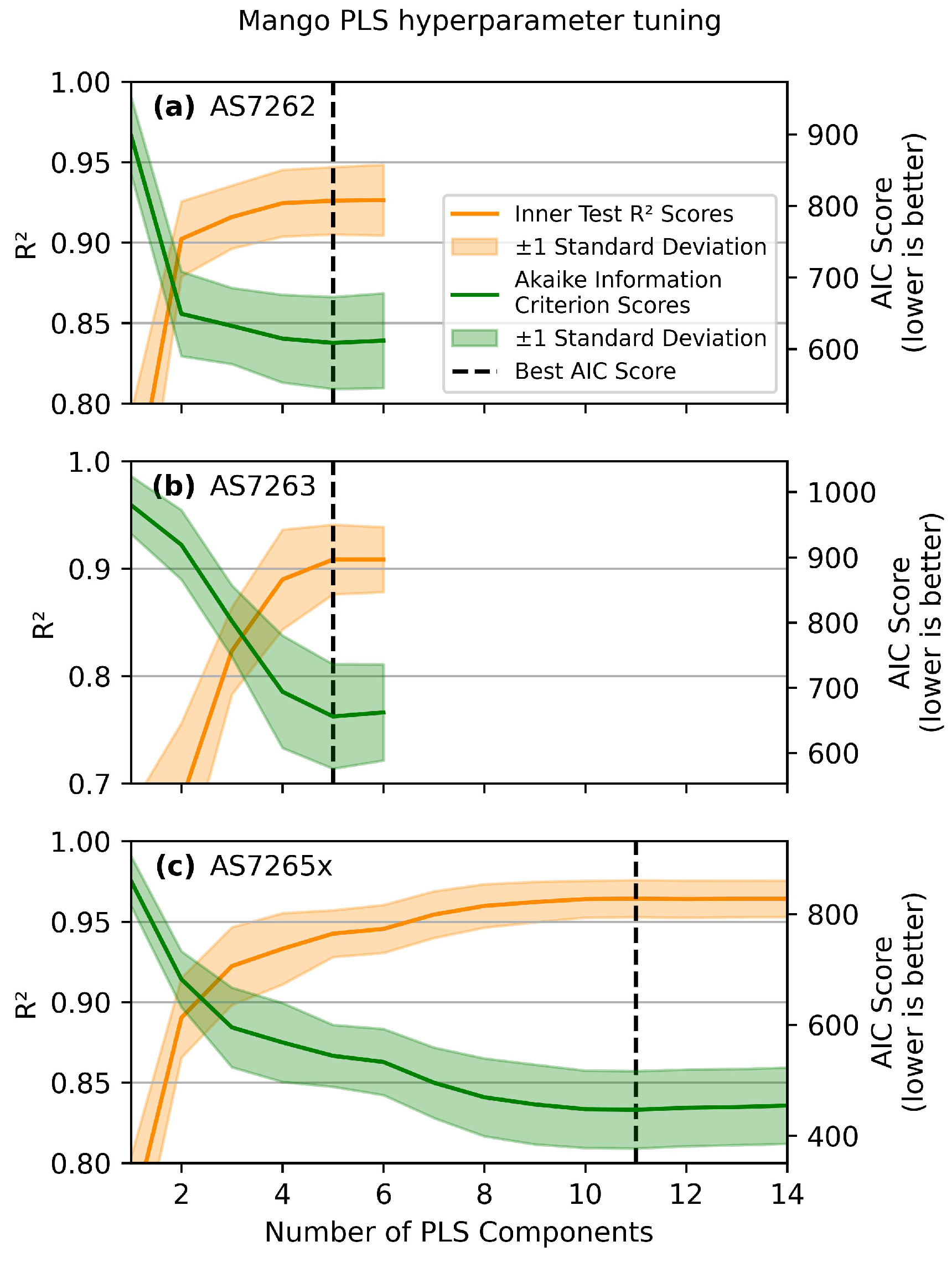
3.3. Model Selection
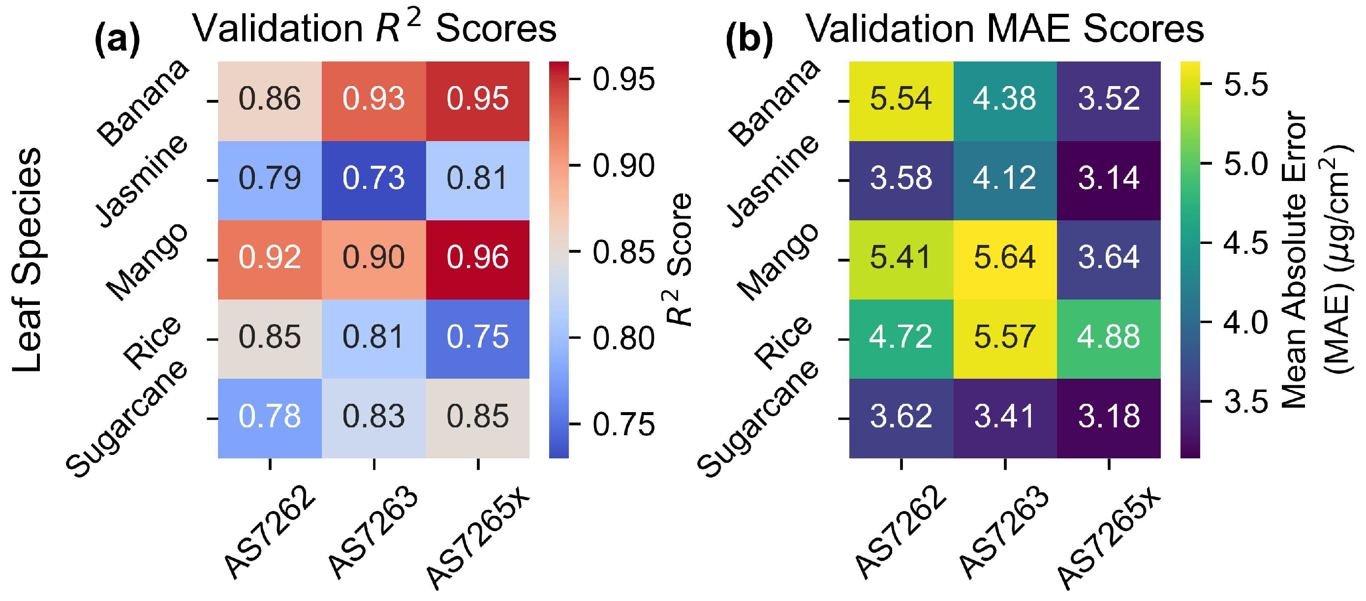
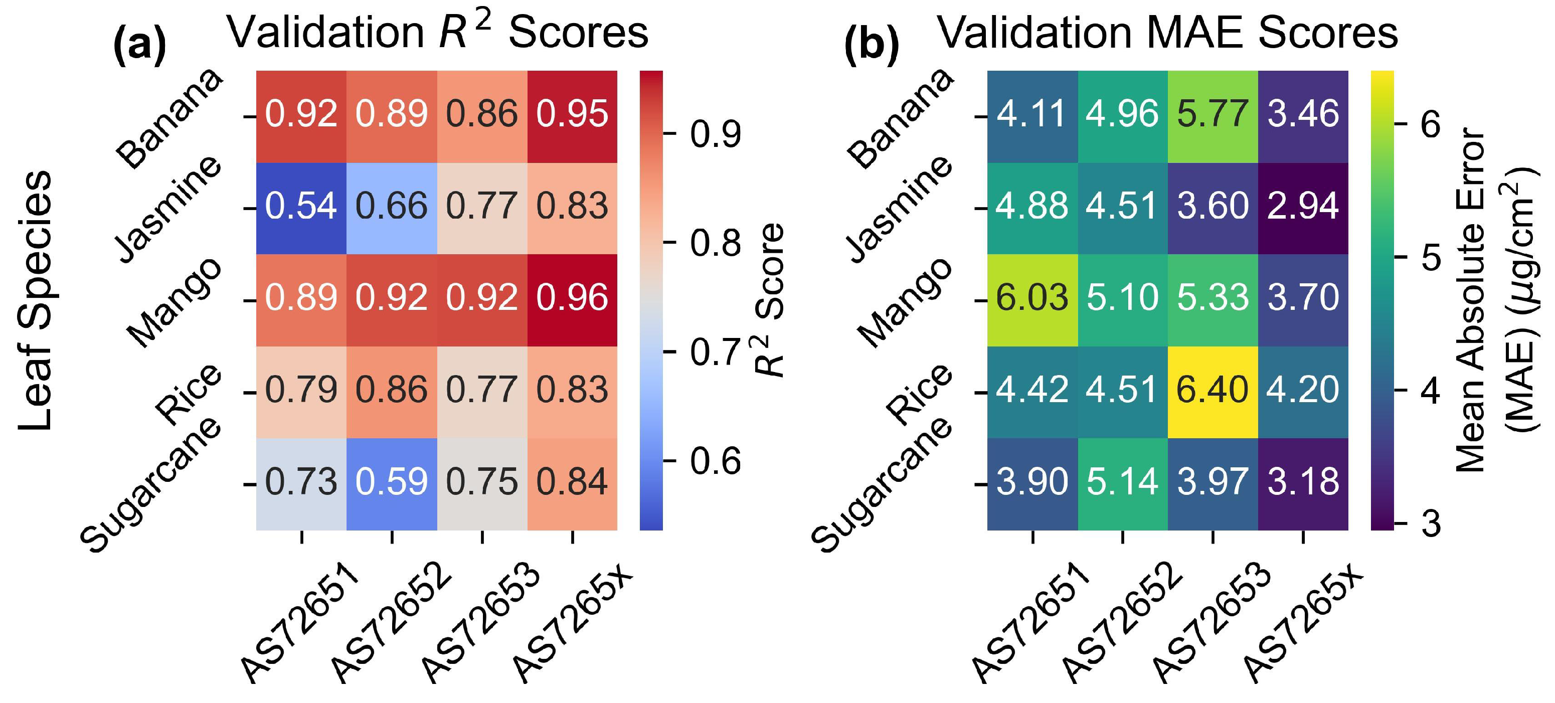
3.4. Validation Scores
3.5. Results by Leaf Species
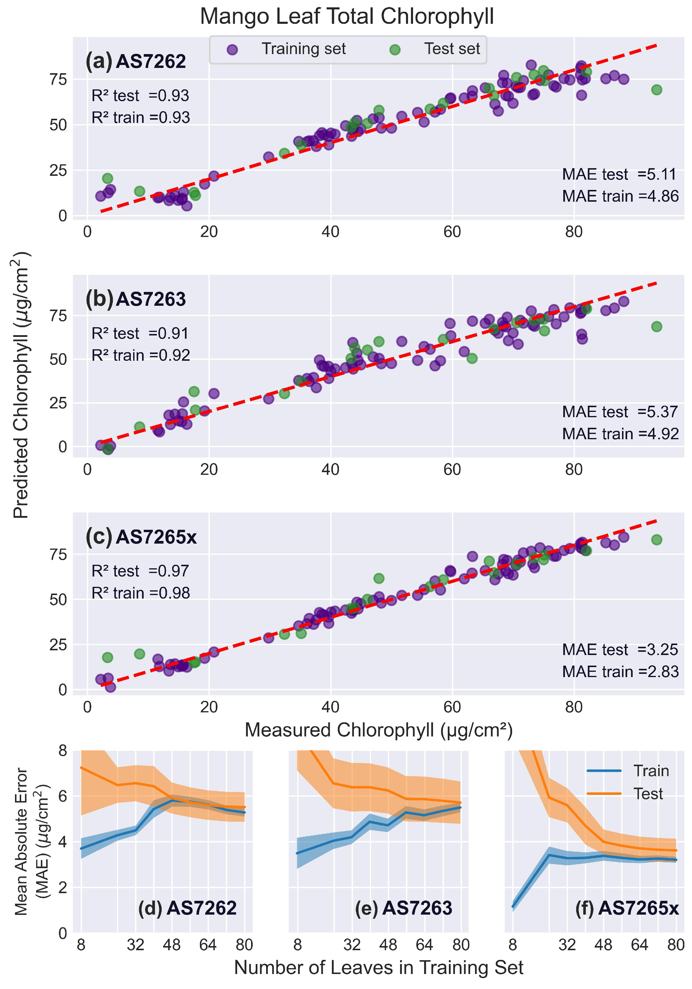
3.5.1. Mango Leaves
3.5.2. Banana Leaves
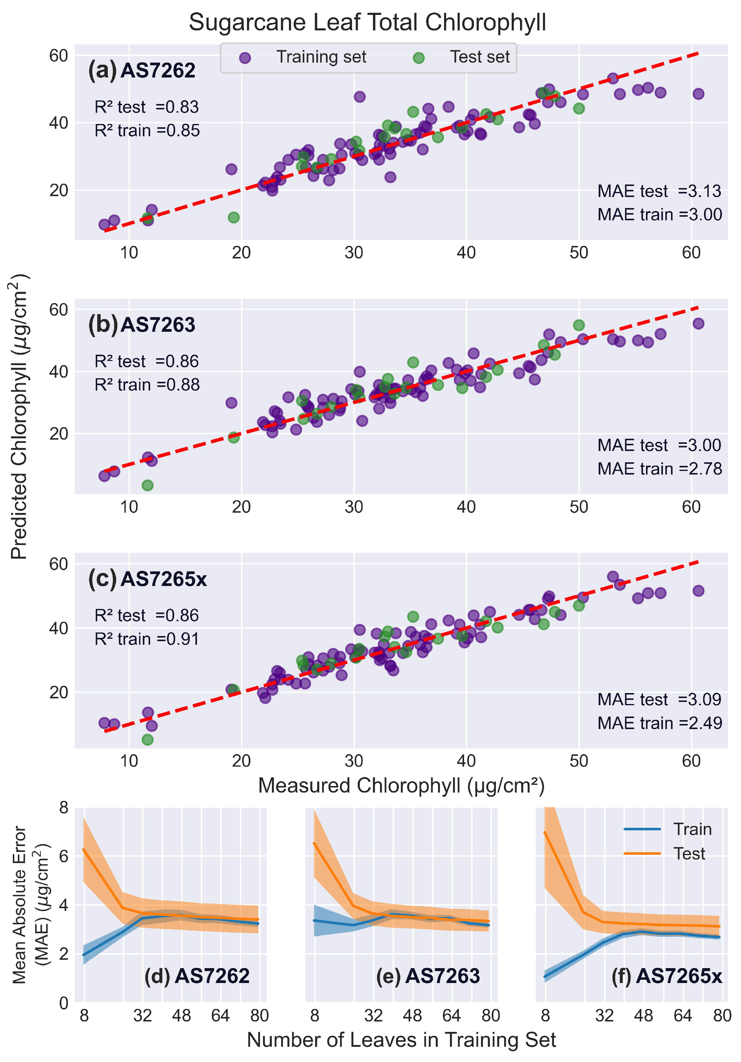
3.5.3. Sugarcane Leaves
3.5.4. Jasmine Leaves
3.5.5. Rice Leaves
4. Discussion
4.1. Sensor Setup and Characterization
4.2. Data Preparation and Model Selection
4.3. Sensor Performance
4.4. Overall Performance and Limitations
5. Conclusions
Supplementary Materials
Author Contributions
Funding
Institutional Review Board Statement
Informed Consent Statement
Data Availability Statement
Conflicts of Interest
References
- Chaudhary, D.R.; Saxena, J.; Lorenz, N.; Dick, R.P. Distribution of Recently Fixed Photosynthate in a Switchgrass Plant-Soil System. Plant Soil Environ. 2012, 58, 249–255. [Google Scholar] [CrossRef]
- Fisher, J.B.; Sitch, S.; Malhi, Y.; Fisher, R.A.; Huntingford, C.; Tan, S.Y. Carbon Cost of Plant Nitrogen Acquisition: A Mechanistic, Globally Applicable Model of Plant Nitrogen Uptake, Retranslocation, and Fixation. Glob. Biogeochem. Cycles 2010, 24, 2009GB003621. [Google Scholar] [CrossRef]
- Ye, X.; Abe, S.; Zhang, S. Estimation and Mapping of Nitrogen Content in Apple Trees at Leaf and Canopy Levels Using Hyperspectral Imaging. Precis. Agric. 2020, 21, 198–225. [Google Scholar] [CrossRef]
- Ustin, S.L.; Jacquemoud, S. How the Optical Properties of Leaves Modify the Absorption and Scattering of Energy and Enhance Leaf Functionality. In Remote Sensing of Plant Biodiversity; Cavender-Bares, J., Gamon, J.A., Townsend, P.A., Eds.; Springer International Publishing: Cham, Switzerland, 2020; pp. 349–384. [Google Scholar] [CrossRef]
- Brown, L.A.; Ogutu, B.O.; Dash, J. Estimating Forest Leaf Area Index and Canopy Chlorophyll Content with Sentinel-2: An Evaluation of Two Hybrid Retrieval Algorithms. Remote Sens. 2019, 11, 1752. [Google Scholar] [CrossRef]
- Ryu, J.H. UAS-based Real-Time Water Quality Monitoring, Sampling, and Visualization Platform (UASWQP). HardwareX 2022, 11, e00277. [Google Scholar] [CrossRef]
- Scutelnic, D.; Muradore, R.; Daffara, C. A Multispectral Camera in the VIS–NIR Equipped with Thermal Imaging and Environmental Sensors for Non Invasive Analysis in Precision Agriculture. HardwareX 2024, 20, e00596. [Google Scholar] [CrossRef]
- Fiorentini, M.; Zenobi, S.; Giorgini, E.; Basili, D.; Conti, C.; Pro, C.; Monaci, E.; Orsini, R. Nitrogen and Chlorophyll Status Determination in Durum Wheat as Influenced by Fertilization and Soil Management: Preliminary Results. PLoS ONE 2019, 14, e0225126. [Google Scholar] [CrossRef]
- Saha, P.; Nayak, H.; Barman, A.; Bera, A.; Banerjee, P. Nitrogen Management by Small Farmers with the Use of Leaf Color Chart: A Review. J. Plant Nutr. 2023, 46, 1836–1844. [Google Scholar]
- Dunn, B.L.; Singh, H.; Payton, M.; Kincheloe, S. Effects of Nitrogen, Phosphorus, and Potassium on SPAD-502 and atLEAF Sensor Readings of Salvia. J. Plant Nutr. 2018, 41, 1674–1683. [Google Scholar] [CrossRef]
- Novichonok, E.V.; Novichonok, A.O.; Kurbatova, J.A.; Markovskaya, E.F. Use of the atLEAF+ Chlorophyll Meter for a Nondestructive Estimate of Chlorophyll Content. Photosynthetica 2016, 54, 130–137. [Google Scholar] [CrossRef]
- Zsebo, S.; Bede, L.; Kukorelli, G.; Kulmány, I.M.; Milics, G.; Stencinger, D.; Teschner, G.; Varga, Z.; Vona, V.; Kovács, A.J. Yield Prediction Using NDVI Values from GreenSeeker and MicaSense Cameras at Different Stages of Winter Wheat Phenology. Drones 2024, 8, 88. [Google Scholar] [CrossRef]
- Ata-Ul-Karim, S.T.; Cao, Q.; Zhu, Y.; Tang, L.; Rehmani, M.I.A.; Cao, W. Non-Destructive Assessment of Plant Nitrogen Parameters Using Leaf Chlorophyll Measurements in Rice. Front. Plant Sci. 2016, 7, 1829. [Google Scholar] [CrossRef] [PubMed]
- Chivenge, P.; Zingore, S.; Ezui, K.S.; Njoroge, S.; Bunquin, M.A.; Dobermann, A.; Saito, K. Progress in Research on Site-Specific Nutrient Management for Smallholder Farmers in Sub-Saharan Africa. Field Crops Res. 2022, 281, 108503. [Google Scholar] [CrossRef]
- Schnitkey, G.; Paulson, N.; Zulauf, C.; Swanson, K.; Colussi, J.; Baltz, A.J. Nitrogen Fertilizer Prices and Supply in Light of the Ukraine-Russia Conflict. Farmdoc Dly. 2022, 12, 45. [Google Scholar]
- Hollister, J.W.; Kellogg, D.Q.; Lei-Parent, Q.; Wilson, E.; Chadwick, C.; Dickson, D.; Gold, A.; Arnold, C. Nsink: An R Package for Flow Path Nitrogen Removal Estimation. J. Open Source Softw. 2022, 7, 4039. [Google Scholar] [CrossRef] [PubMed]
- Maaz, T.M.; Sapkota, T.B.; Eagle, A.J.; Kantar, M.B.; Bruulsema, T.W.; Majumdar, K. Meta-Analysis of Yield and Nitrous Oxide Outcomes for Nitrogen Management in Agriculture. Glob. Change Biol. 2021, 27, 2343–2360. [Google Scholar] [CrossRef]
- Albornoz, F. Crop Responses to Nitrogen Overfertilization: A Review. Sci. Hortic. 2016, 205, 79–83. [Google Scholar] [CrossRef]
- Kong, L.; Xie, Y.; Hu, L.; Si, J.; Wang, Z. Excessive Nitrogen Application Dampens Antioxidant Capacity and Grain Filling in Wheat as Revealed by Metabolic and Physiological Analyses. Sci. Rep. 2017, 7, 43363. [Google Scholar] [CrossRef]
- Mittermayer, M.; Gilg, A.; Maidl, F.X.; Nätscher, L.; Hülsbergen, K.J. Site-specific Nitrogen Balances Based on Spatially Variable Soil and Plant Properties. Precis. Agric. 2021, 22, 1416–1436. [Google Scholar] [CrossRef]
- Franzen, D.; Kitchen, N.; Holland, K.; Schepers, J.; Raun, W. Algorithms for In-Season Nutrient Management in Cereals. Agron. J. 2016, 108, 1775–1781. [Google Scholar] [CrossRef]
- Rudnick, J.; Lubell, M.; Khalsa, S.D.S.; Tatge, S.; Wood, L.; Sears, M.; Brown, P.H. A Farm Systems Approach to the Adoption of Sustainable Nitrogen Management Practices in California. Agric. Hum. Values 2021, 38, 783–801. [Google Scholar] [CrossRef]
- Wang, J.; Shi, X.; Xu, Y.; Dong, C. Nitrogen Management Based on Visible/Near Infrared Spectroscopy in Pear Orchards. Remote Sens. 2021, 13, 927. [Google Scholar] [CrossRef]
- Cao, Q.; Miao, Y.; Shen, J.; Yu, W.; Yuan, F.; Cheng, S.; Huang, S.; Wang, H.; Yang, W.; Liu, F. Improving In-Season Estimation of Rice Yield Potential and Responsiveness to Topdressing Nitrogen Application with Crop Circle Active Crop Canopy Sensor. Precis. Agric. 2016, 17, 136–154. [Google Scholar] [CrossRef]
- Saudy, H.S. Chlorophyll Meter as a Tool for Forecasting Wheat Nitrogen Requirements after Application of Herbicides. Arch. Agron. Soil Sci. 2014, 60, 1077–1090. [Google Scholar] [CrossRef]
- Ghosh, M.; Roychowdhury, A.; Dutta, S.K.; Hazra, K.K.; Singh, G.; Kohli, A.; Kumar, S.; Acharya, S.; Mandal, J.; Singh, Y.K.; et al. SPAD Chlorophyll Meter-Based Real-Time Nitrogen Management in Manure-Amended Lowland Rice. J. Soil Sci. Plant Nutr. 2023, 23, 5993–6005. [Google Scholar] [CrossRef]
- Bijay-Singh; Ali, A.M. Using Hand-Held Chlorophyll Meters and Canopy Reflectance Sensors for Fertilizer Nitrogen Management in Cereals in Small Farms in Developing Countries. Sensors 2020, 20, 1127. [Google Scholar] [CrossRef]
- Ali, A.M.; Salem, H.M.; Bijay-Singh. Site-Specific Nitrogen Fertilizer Management Using Canopy Reflectance Sensors, Chlorophyll Meters and Leaf Color Charts: A Review. Nitrogen 2024, 5, 828–856. [Google Scholar] [CrossRef]
- Lesiv, M.; Laso Bayas, J.C.; See, L.; Duerauer, M.; Dahlia, D.; Durando, N.; Hazarika, R.; Kumar Sahariah, P.; Vakolyuk, M.; Blyshchyk, V.; et al. Estimating the Global Distribution of Field Size Using Crowdsourcing. Glob. Change Biol. 2019, 25, 174–186. [Google Scholar] [CrossRef]
- Ren, C.; Liu, S.; van Grinsven, H.; Reis, S.; Jin, S.; Liu, H.; Gu, B. The Impact of Farm Size on Agricultural Sustainability. J. Clean. Prod. 2019, 220, 357–367. [Google Scholar] [CrossRef]
- Wu, Y.; Xi, X.; Tang, X.; Luo, D.; Gu, B.; Lam, S.K.; Vitousek, P.M.; Chen, D. Policy Distortions, Farm Size, and the Overuse of Agricultural Chemicals in China. Proc. Natl. Acad. Sci. USA 2018, 115, 7010–7015. [Google Scholar] [CrossRef]
- Ospino-Villalba, K.; Gaviria, D.; Pineda, D.; Pérez, J. A 3D-Printable Smartphone Accessory for Plant Leaf Chlorophyll Measurement. HardwareX 2024, 20, e00597. [Google Scholar] [CrossRef]
- Hassanijalilian, O.; Igathinathane, C.; Doetkott, C.; Bajwa, S.; Nowatzki, J.; Haji Esmaeili, S.A. Chlorophyll Estimation in Soybean Leaves Infield with Smartphone Digital Imaging and Machine Learning. Comput. Electron. Agric. 2020, 174, 105433. [Google Scholar] [CrossRef]
- Sala, F.; Herbei, M.V. Evaluation of Different Methods and Models for Grass Cereals’ Production Estimation: Case Study in Wheat. Agronomy 2023, 13, 1500. [Google Scholar] [CrossRef]
- Kamarianakis, Z.; Panagiotakis, S. Design and Implementation of a Low-Cost Chlorophyll Content Meter. Sensors 2023, 23, 2699. [Google Scholar] [CrossRef] [PubMed]
- Andrianto, H.; Suhardi, S.; Faizal, A. Performance Evaluation of Low-Cost IoT Based Chlorophyll Meter. Bull. Electr. Eng. Inform. 2020, 9, 956–963. [Google Scholar] [CrossRef]
- Putra, B.T.W. New Low-Cost Portable Sensing System Integrated with on-the-Go Fertilizer Application System for Plantation Crops. Measurement 2020, 155, 107562. [Google Scholar]
- Li, L.; Guo, J.; Wang, Q.; Wang, J.; Liu, Y.; Shi, Y. Design and Experiment of a Portable Near-Infrared Spectroscopy Device for Convenient Prediction of Leaf Chlorophyll Content. Sensors 2023, 23, 8585. [Google Scholar] [CrossRef]
- Habibullah, M.; Mohebian, M.R.; Soolanayakanahally, R.; Wahid, K.A.; Dinh, A. A Cost-Effective and Portable Optical Sensor System to Estimate Leaf Nitrogen and Water Contents in Crops. Sensors 2020, 20, 1449. [Google Scholar] [CrossRef]
- Tran, T.N.; Keller, R.; Trinh, V.Q.; Tran, K.Q.; Kaldenhoff, R. Multi-Channel Spectral Sensors as Plant Reflectance Measuring Devices—Toward the Usability of Spectral Sensors for Phenotyping of Sweet Basil (Ocimum Basilicum). Agronomy 2022, 12, 1174. [Google Scholar] [CrossRef]
- Noguera, M.; Millan, B.; Andújar, J.M. New, Low-Cost, Hand-Held Multispectral Device for In-Field Fruit-Ripening Assessment. Agriculture 2023, 13, 4. [Google Scholar] [CrossRef]
- Noguera, M.; Millan, B.; Aquino, A.; Andújar, J.M. Methodology for Olive Fruit Quality Assessment by Means of a Low-Cost Multispectral Device. Agronomy 2022, 12, 979. [Google Scholar] [CrossRef]
- Sulistyo, S.B.; Siswantoro; Margiwiyatno, A.; Masrukhi; Mustofa, A.; Sudarmaji, A.; Ediati, R.; Listanti, R.; Hidayat, H.H. Handheld Arduino-Based near Infrared Spectrometer for Non-Destructive Quality Evaluation of Siamese Oranges. IOP Conf. Ser. Earth Environ. Sci. 2021, 653, 012119. [Google Scholar] [CrossRef]
- Srinivasagan, R.; Mohammed, M.; Alzahrani, A. TinyML-Sensor for Shelf Life Estimation of Fresh Date Fruits. Sensors 2023, 23, 7081. [Google Scholar] [CrossRef] [PubMed]
- Sharma, A.; Kumar, R.; Kumar, N.; Saxena, V. Machine Learning Driven Portable Vis-SWNIR Spectrophotometer for Non-Destructive Classification of Raw Tomatoes Based on Lycopene Content. Vib. Spectrosc. 2024, 130, 103628. [Google Scholar] [CrossRef]
- Sharma, A.; Kumar, R.; Kumar, N.; Kaur, K.; Saxena, V.; Ghosh, P. Chemometrics Driven Portable Vis-SWNIR Spectrophotometer for Non-Destructive Quality Evaluation of Raw Tomatoes. Chemom. Intell. Lab. Syst. 2023, 242, 105001. [Google Scholar] [CrossRef]
- Chen, C.L.; Liao, Y.C.; Fang, M. Freshness Evaluation of Grouper Fillets by Inexpensive E-Nose and Spectroscopy Sensors. Microchem. J. 2024, 198, 110145. [Google Scholar] [CrossRef]
- Sutherland, C.; Henderson, A.D.; Giosio, D.R.; Trotter, A.J.; Smith, G.G. Synchronising an IMX219 Image Sensor and AS7265x Spectral Sensor to Make a Novel Low-Cost Spectral Camera. HardwareX 2024, 19, e00573. [Google Scholar] [CrossRef]
- Stevens, J.D.; Murray, D.; Diepeveen, D.; Toohey, D. Adaptalight: An Inexpensive PAR Sensor System for Daylight Harvesting in a Micro Indoor Smart Hydroponic System. Horticulturae 2022, 8, 105. [Google Scholar] [CrossRef]
- Botero-Valencia, J.S.; Mejia-Herrera, M. Modular System for UV–Vis-NIR Radiation Measurement with Wireless Communication. HardwareX 2021, 10, e00236. [Google Scholar] [CrossRef]
- Chen, S.T.; Ward, C.P.; Long, M.H. Quantifying Pelagic Primary Production and Respiration via an Automated in Situ Incubation System. Limnol. Oceanogr. Methods 2023, 21, 495–507. [Google Scholar] [CrossRef]
- Duncan, L.; Miller, B.; Shaw, C.; Graebner, R.; Moretti, M.L.; Walter, C.; Selker, J.; Udell, C. Weed Warden: A Low-Cost Weed Detection Device Implemented with Spectral Triad Sensor for Agricultural Applications. HardwareX 2022, 11, e00303. [Google Scholar] [CrossRef] [PubMed]
- Moran, R. Formulae for Determination of Chlorophyllous Pigments Extracted with N,N-Dimethylformamide. Plant Physiol. 1982, 69, 1376. [Google Scholar] [CrossRef]
- Yin, L.; Lv, L.; Wang, D.; Qu, Y.; Chen, H.; Deng, W. Spectral Clustering Approach with K-Nearest Neighbor and Weighted Mahalanobis Distance for Data Mining. Electronics 2023, 12, 3284. [Google Scholar] [CrossRef]
- Sáez, J.A.; Romero-Béjar, J.L. Impact of Regressand Stratification in Dataset Shift Caused by Cross-Validation. Mathematics 2022, 10, 2538. [Google Scholar] [CrossRef]
- Karabourniotis, G.; Liakopoulos, G.; Bresta, P.; Nikolopoulos, D. The Optical Properties of Leaf Structural Elements and Their Contribution to Photosynthetic Performance and Photoprotection. Plants 2021, 10, 1455. [Google Scholar] [CrossRef]
- Sukhova, E.; Zolin, Y.; Grebneva, K.; Berezina, E.; Bondarev, O.; Kior, A.; Popova, A.; Ratnitsyna, D.; Yudina, L.; Sukhov, V. Development of Analytical Model to Describe Reflectance Spectra in Leaves with Palisade and Spongy Mesophyll. Plants 2024, 13, 3258. [Google Scholar] [CrossRef]
- Yuan, K.H.; Fung, W.K.; Reise, S.P. Three Mahalanobis Distances and Their Role in Assessing Unidimensionality. Br. J. Math. Stat. Psychol. 2004, 57, 151–165. [Google Scholar] [CrossRef]
- Akhtar, N.; Hayat, M.Q.; Habib, U.; Khan, M.A.; Malik, S.I.; Hafeez, H.; Hussain, A.; Hussain, A.; Potter, D. Comparative Taxonomy and Evolutionary Significance of Foliar Epidermis in Jasminum L. (Oleaceae) Based on Light and Scanning Electron Microscopy. Flora 2024, 310, 152419. [Google Scholar] [CrossRef]
- Aho, K.; Derryberry, D.; Peterson, T. Model Selection for Ecologists: The Worldviews of AIC and BIC. Ecology 2014, 95, 631–636. [Google Scholar] [CrossRef] [PubMed]
- Krstajic, D.; Buturovic, L.J.; Leahy, D.E.; Thomas, S. Cross-Validation Pitfalls When Selecting and Assessing Regression and Classification Models. J. Cheminform. 2014, 6, 10. [Google Scholar] [CrossRef]
- Michelucci, U.; Venturini, F. New Metric Formulas That Include Measurement Errors in Machine Learning for Natural Sciences. Expert Syst. Appl. 2023, 224, 120013. [Google Scholar] [CrossRef]
- Acevedo-Correa, C.; Goez, M.; Torres-Madronero, M.C.; Rondon, T. Low-Cost Clamp for the Measurement of Vegetation Spectral Signatures. HardwareX 2024, 19, e00557. [Google Scholar] [CrossRef] [PubMed]
- Tunens, G.; Einbergs, E.; Laganovska, K.; Zolotarjovs, A.; Vilks, K.; Skuja, L.; Smits, K. Optical Fiber-Based Open Source Low Cost Portable Spectrometer System. HardwareX 2024, 18, e00530. [Google Scholar] [CrossRef]
- Nengsih, T.A.; Bertrand, F.; Maumy-Bertrand, M.; Meyer, N. Determining the Number of Components in PLS Regression on Incomplete Data. Stat. Appl. Genet. Mol. Biol. 2019, 18, 20180059. [Google Scholar] [CrossRef]
- Brown, L.A.; Williams, O.; Dash, J. Calibration and Characterisation of Four Chlorophyll Meters and Transmittance Spectroscopy for Non-Destructive Estimation of Forest Leaf Chlorophyll Concentration. Agric. For. Meteorol. 2022, 323, 109059. [Google Scholar] [CrossRef]
- Donnelly, A.; Yu, R.; Rehberg, C.; Meyer, G.A.; Young, E.B. Leaf Chlorophyll Estimates of Temperate Deciduous Shrubs during Autumn Senescence Using a SPAD-502 Meter and Calibration with Extracted Chlorophyll. Ann. For. Sci. 2020, 77, 1–12. [Google Scholar]
- Pandey, S.; Tyagi, D. Changes in Chlorophyll Content and Photosynthetic Rate of Four Cultivars of Mango during Reproductive Phase. Biol. Plant. 1999, 42, 457–461. [Google Scholar] [CrossRef]
- Ganeshamurthy, A.N.; Rupa, T.R.; Shivananda, T.N. Enhancing Mango Productivity through Sustainable Resource Management. J. Hortic. Sci. 2018, 13, 1–31. [Google Scholar]
- Mahajan, G.R.; Das, B.; Murgaokar, D.; Herrmann, I.; Berger, K.; Sahoo, R.N.; Patel, K.; Desai, A.; Morajkar, S.; Kulkarni, R.M. Monitoring the Foliar Nutrients Status of Mango Using Spectroscopy-Based Spectral Indices and PLSR-Combined Machine Learning Models. Remote Sens. 2021, 13, 641. [Google Scholar] [CrossRef]
- Abro, B.A.; Memon, M.; Hassan, Z.U.; Arain, M.Y.; Razaq, A.; Abro, D.A.; Ali, S. Assessing Nitrogen Nutrition of Banana Basrai (Dwarf Cavendish) through Leaf Analysis and Chlorophyll Determination. Pak. J. Bot. 2021, 31, 1859–1864. [Google Scholar] [CrossRef]
- Rabatel, G.; Lamour, J.; Moura, D.; Naud, O. A Multispectral Processing Chain for Chlorophyll Content Assessment in Banana Fields by UAV Imagery. In Precision Agriculture’19; Wageningen Academic: Wageningen, The Netherlands, 2019; pp. 413–419. [Google Scholar]
- Kan, B.; Yang, Y.; Du, P.; Li, X.; Lai, W.; Hu, H. Chlorophyll Decomposition Is Accelerated in Banana Leaves after the Long-Term Magnesium Deficiency According to Transcriptome Analysis. PLoS ONE 2022, 17, e0270610. [Google Scholar] [CrossRef]
- Meghwal, M.L.; Jyothi, M.L.; Pushpalatha, P.B.; Bhaskar, J.; Beena, V.I.; Thulasi, V. Influence of Nutrient Sources on Chlorophyll Content and Other Leaf Parameters of Banana Musa (AAB) Nendran. Agric. Sci. Dig. 2021, 44, 118–121. [Google Scholar]
- Radhamani, R.; Kannan, R.; Rakkiyappan, P. Leaf Chlorophyll Meter Readings as an Indicator for Sugarcane Yield Under Iron Deficient Typic Haplustert. Sugar Tech 2016, 18, 61–66. [Google Scholar] [CrossRef]
- Harakotr, P.; Sornpha, W.; Khonghintaisong, J.; Gonkhamdee, S.; Songsri, P.; Jongrungklang, N. Correlation between Rapid Measurement and Leaf Chlorophyll Content of Various Sugarcane Genotypes at Different Growth Phases. Asian J. Plant Sci. 2024, 23, 367–376. [Google Scholar] [CrossRef]
- Martins, J.A.; Fiorio, P.R.; Barros, P.P.d.S.; Demattê, J.A.M.; Molin, J.P.; Cantarella, H.; Neale, C.M.U. Potential Use of Hyperspectral Data to Monitor Sugarcane Nitrogen Status. Acta Sci. Agron. 2020, 43, e47632. [Google Scholar]
- Parry, C.; Blonquist, J.M., Jr.; Bugbee, B. In Situ Measurement of Leaf Chlorophyll Concentration: Analysis of the Optical/Absolute Relationship. Plant Cell Environ. 2014, 37, 2508–2520. [Google Scholar] [CrossRef]
- Behera, S.D.; Garnayak, L.M.; Behera, B.; Panda, R.K. Chlorophyll Content and SPAD Value Relationships Between Varying Nitrogen Application and Cultivar in Rice. J. Indian Soc. Coast. Agric. Res. 2022, 40, 23–30. [Google Scholar] [CrossRef]
- Zhang, J.; Wan, L.; Igathinathane, C.; Zhang, Z.; Guo, Y.; Sun, D.; Cen, H. Spatiotemporal Heterogeneity of Chlorophyll Content and Fluorescence Response Within Rice (Oryza Sativa L.) Canopies Under Different Nitrogen Treatments. Front. Plant Sci. 2021, 12, 645977. [Google Scholar] [CrossRef]
- Ali, A.M.; Thind, H.S.; Sharma, S.; Singh, Y. Site-Specific Nitrogen Management in Dry Direct-Seeded Rice Using Chlorophyll Meter and Leaf Colour Chart. Pedosphere 2015, 25, 72–81. [Google Scholar] [CrossRef]


| AS7262 | AS7263 | AS7265x | |
|---|---|---|---|
| Banana | 6 | 5 | 8 |
| Jasmine | 4 | 5 | 14 |
| Mango | 5 | 5 | 11 |
| Rice | 6 | 5 | 6 |
| Sugarcane | 6 | 5 | 6 |
Disclaimer/Publisher’s Note: The statements, opinions and data contained in all publications are solely those of the individual author(s) and contributor(s) and not of MDPI and/or the editor(s). MDPI and/or the editor(s) disclaim responsibility for any injury to people or property resulting from any ideas, methods, instructions or products referred to in the content. |
© 2025 by the authors. Licensee MDPI, Basel, Switzerland. This article is an open access article distributed under the terms and conditions of the Creative Commons Attribution (CC BY) license (https://creativecommons.org/licenses/by/4.0/).
Share and Cite
Lopin, P.; Nawsang, P.; Laywisadkul, S.; Lopin, K.V. Evaluation of Low-Cost Multi-Spectral Sensors for Measuring Chlorophyll Levels Across Diverse Leaf Types. Sensors 2025, 25, 2198. https://doi.org/10.3390/s25072198
Lopin P, Nawsang P, Laywisadkul S, Lopin KV. Evaluation of Low-Cost Multi-Spectral Sensors for Measuring Chlorophyll Levels Across Diverse Leaf Types. Sensors. 2025; 25(7):2198. https://doi.org/10.3390/s25072198
Chicago/Turabian StyleLopin, Prattana, Pichapob Nawsang, Srisangwan Laywisadkul, and Kyle V. Lopin. 2025. "Evaluation of Low-Cost Multi-Spectral Sensors for Measuring Chlorophyll Levels Across Diverse Leaf Types" Sensors 25, no. 7: 2198. https://doi.org/10.3390/s25072198
APA StyleLopin, P., Nawsang, P., Laywisadkul, S., & Lopin, K. V. (2025). Evaluation of Low-Cost Multi-Spectral Sensors for Measuring Chlorophyll Levels Across Diverse Leaf Types. Sensors, 25(7), 2198. https://doi.org/10.3390/s25072198