
Prescribed Performance Bounded-H∞ Control for Flexible-Joint Manipulators Without Initial Condition Restriction


Abstract
1. Introduction
2. Problem Formulation and Preliminaries
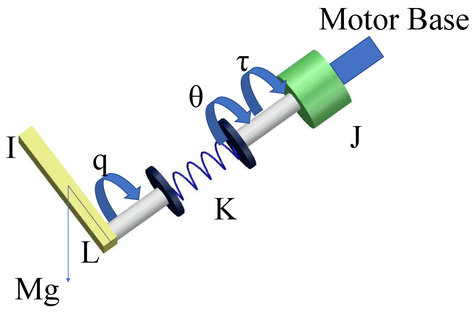
2.1. Plant Formulation
2.2. Preliminaries
- 1.
- .
- 2.
- .
2.3. Prescribed Performance Control
3. Controller Design and Stability Analysis
- 1.
- The output remains within the prescribed performance boundaries specified by the PFTPF when .
- 2.
- The system exhibits H∞ disturbance attenuation performance for external disturbances.
- 3.
- All signals in the system are bounded.
- Proof of prescribed performance:According to (65) and Lemma (1), it follows that is bounded. Furthermore, because and as well as , the prescribed performance is achieved.Furthermore, the output of the SLFJM enters the range when and the range when . Thus, the prescribed performance is guaranteed.
- Stability analysis:Because of the continuity of the output signal, is bounded. Consequently, and z are bounded. Similarly, is bounded.Furthermore, from the control laws, . Thus, is bounded.According to (19), it follows that is bounded. Similarly, u is bounded.This completes the stability analysis of the system.
- Proof of bounded-H∞ disturbance attenuation performance:Define an auxiliary Lyapunov function aswhere is a positive constant applied in H∞ disturbance attenuation performance. is introduced to ensure that . The boundness of the system shows that the number exists.Define an auxiliary functionwhere .Invoking (67) into (65), we can obtain a positive constant h, ensuringwhere . The h is defined to prove the bounded-H∞ performance of the system. In addition, h has no physical meaning in the real world and does not join the designing of the controller.In addition,Therefore, (70) can also be expressed aswhere .According to the Gronwall’s inequality, it can be deduced thatNext, we present a proof of contradiction to demonstrate that .If , thenThus, , and we conclude thatApplying Gronwall’s inequality and noting that , we obtainwhich means thatwhere . Therefore, the system satisfies the performance index defined in Definition 1, completing the proof of Theorem 2.
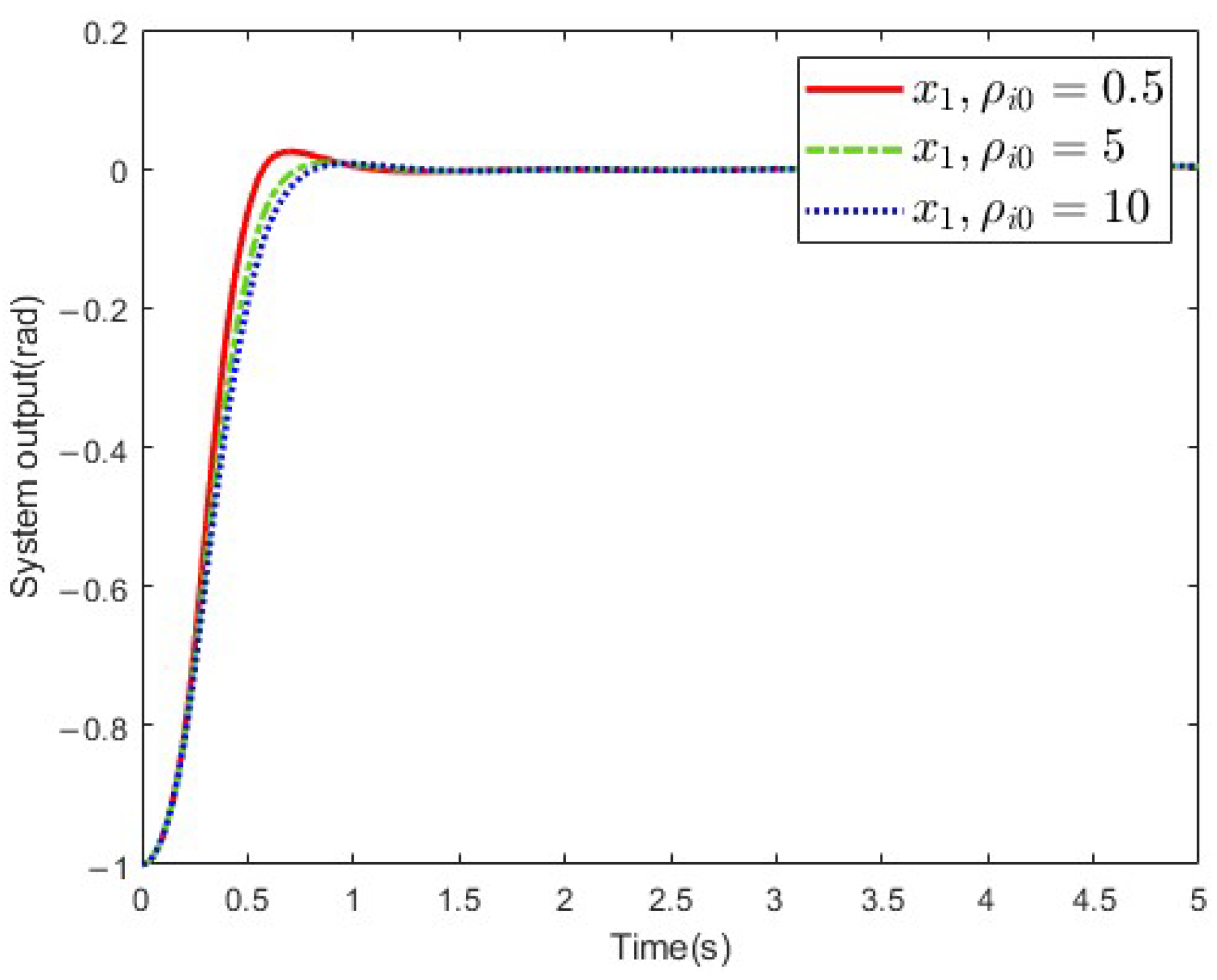
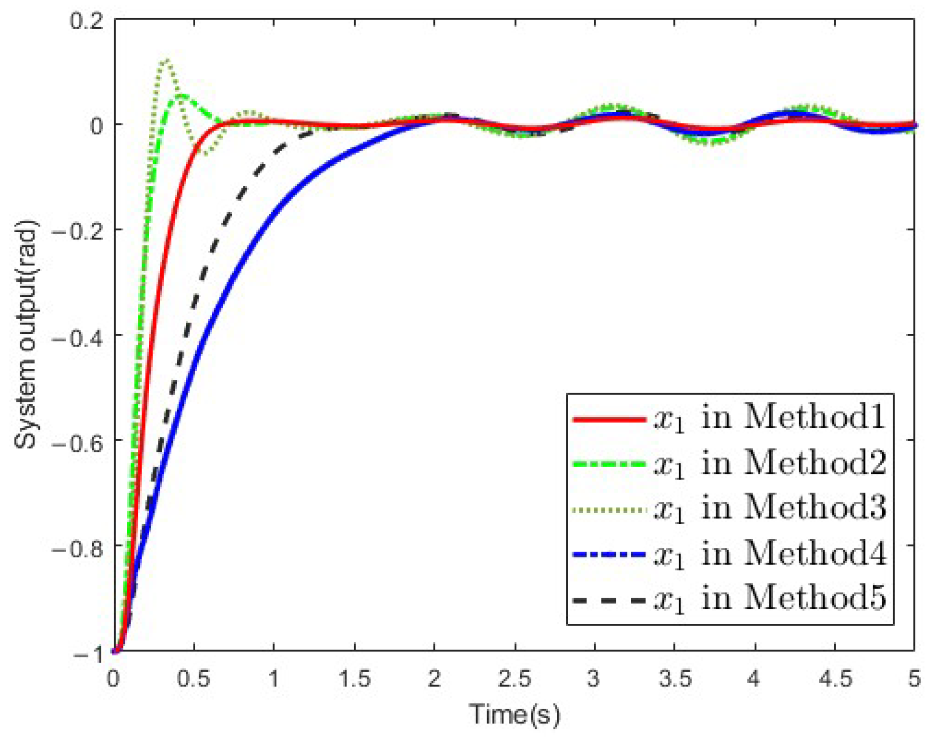
4. Simulation
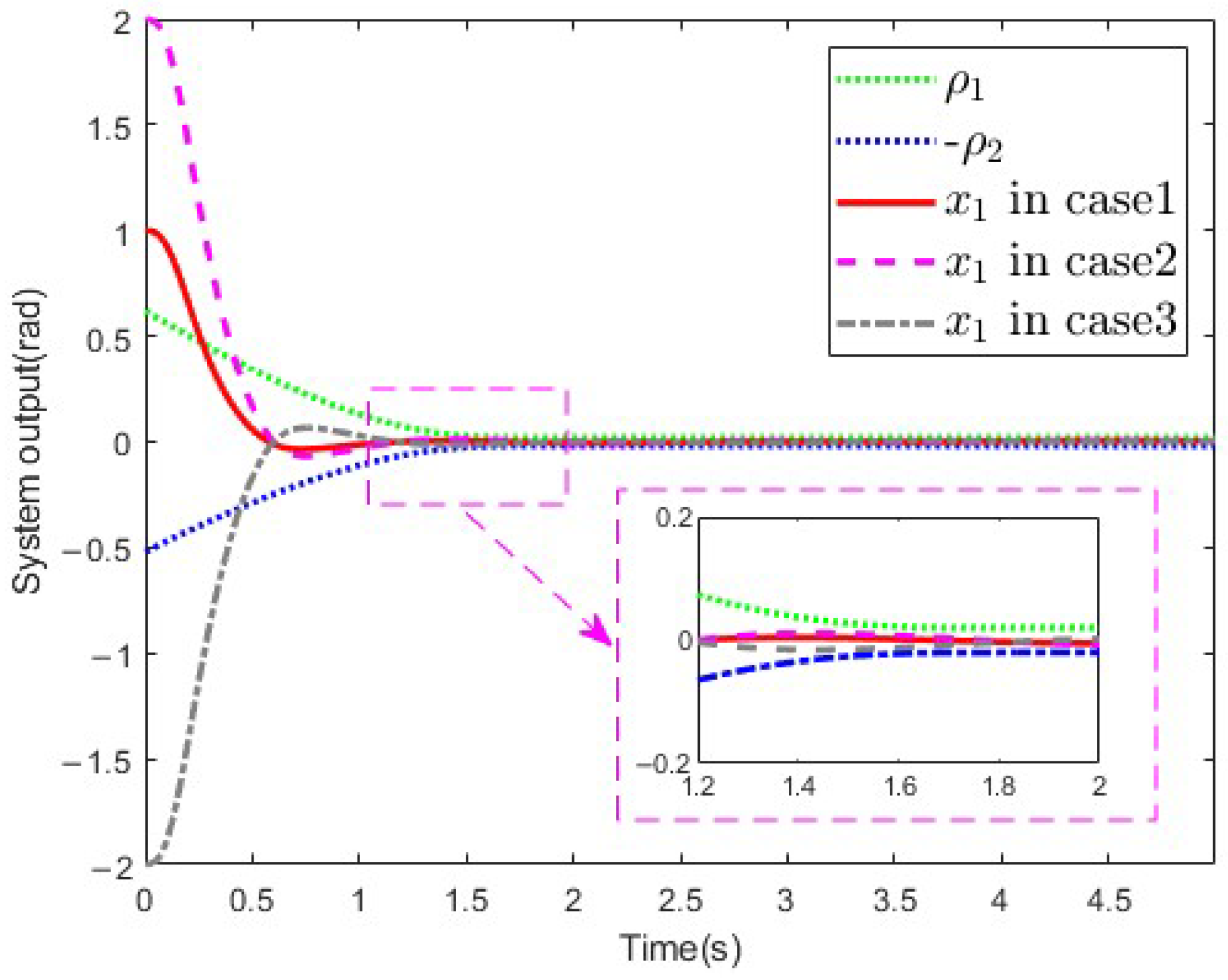
- Case 1: ;
- Case 2: ;
- Case 3: .
5. Conclusions
Author Contributions
Funding
Institutional Review Board Statement
Informed Consent Statement
Data Availability Statement
Acknowledgments
Conflicts of Interest
Abbreviations
| SLMFJ | single-link flexible-joint manipulator |
| PPC | prescribed performance function |
| BLF | barrier Lyapunov function |
| ICF | input control function |
| IEF | initial expansion function |
References
- Bilal, H.; Yin, B.; Aslam, M.S.; Anjum, Z.; Rohra, A.; Wang, Y. A practical study of active disturbance rejection control for rotary flexible joint robot manipulator. Soft Comput. 2023, 27, 4987–5001. [Google Scholar] [CrossRef]
- Tian, G.; Tan, J.; Li, B.; Duan, G. Optimal fully actuated system approach-based trajectory tracking control for robot manipulators. IEEE Trans. Cybern. 2024, 54, 7469–7478. [Google Scholar] [CrossRef]
- Alves, S.; Babcinschi, M.; Silva, A.; Neto, D.; Fonseca, D.; Neto, P. Integrated design fabrication and control of a bioinspired multimaterial soft robotic hand. Cyborg Bionic Syst. 2023, 4, 0051. [Google Scholar]
- Gao, Q.; Deng, Z.; Ju, Z.; Zhang, T. Dual-hand motion capture by using biological inspiration for bionic bimanual robot teleoperation. Cyborg Bionic Syst. 2023, 4, 0052. [Google Scholar]
- Xing, X.; Qin, L.; Luo, Y.; Feng, L.; Xiao, B. Prescribed Performance Backstepping Attitude Control of Parafoil System for Rocket Booster Recovery Under Complex Unknown Disturbances. IEEE Trans. Aerosp. Electron. Syst. 2025, 61, 620–631. [Google Scholar]
- Wang, F.; Chen, K.; Zhen, S.; Chen, X.; Zheng, H.; Wang, Z. Prescribed performance adaptive robust control for robotic manipulators with fuzzy uncertainty. IEEE Trans. Fuzzy Syst. 2023, 32, 1318–1330. [Google Scholar]
- Qi, H.; Ding, L.; Zheng, M.; Huang, L.; Gao, H.; Liu, G.; Deng, Z. Variable Wheelbase Control of Wheeled Mobile Robots with Worm-Inspired Creeping Gait Strategy. IEEE Trans. Robot. 2024, 40, 3271–3289. [Google Scholar]
- Pradhan, S.K.; Subudhi, B. Position control of a flexible manipulator using a new nonlinear self-tuning PID controller. IEEE/CAA J. Autom. Sin. 2020, 7, 136–149. [Google Scholar]
- Moyrón, J.; Moreno-Valenzuela, J.; Sandoval, J. Global Regulation of Flexible Joint Robots with Input Saturation by Nonlinear I-PID-Type Control. IEEE Trans. Control Syst. Technol. 2024, 32, 2385–2393. [Google Scholar] [CrossRef]
- Zheng, S.; Ahn, C.K.; Wan, M.; Xie, Y.; Shi, P. Adaptive Cooperative Output Regulation for Multiple Flexible Manipulators. IEEE Trans. Syst. Man Cybern. Syst. 2024, 54, 4819–4831. [Google Scholar]
- Rsetam, K.; Cao, Z.; Wang, L.; Al-Rawi, M.; Man, Z. Practically robust fixed-time convergent sliding mode control for underactuated aerial flexible jointrobots manipulators. Drones 2022, 6, 428. [Google Scholar] [CrossRef]
- Zhan, B.; Jin, M.; Liu, J. Extended-state-observer-based adaptive control of flexible-joint space manipulators with system uncertainties. Adv. Space Res. 2022, 69, 3088–3102. [Google Scholar]
- Hong, M.; Gu, X.; Liu, L.; Guo, Y. Finite time extended state observer based nonsingular fast terminal sliding mode control of flexible-joint manipulators with unknown disturbance. J. Frankl. Inst. 2023, 360, 18–37. [Google Scholar]
- Bechlioulis, C.P.; Rovithakis, G.A. Prescribed performance adaptive control of SISO feedback linearizable systems with disturbances. In Proceedings of the 2008 16th Mediterranean Conference on Control and Automation, Ajaccio, France, 25–27 June 2008; IEEE: Piscataway, NJ, USA, 2008; pp. 1035–1040. [Google Scholar]
- Xu, F.; Tang, L.; Liu, Y.J. Tangent barrier Lyapunov function-based constrained control of flexible manipulator system with actuator failure. Int. J. Robust Nonlinear Control 2021, 31, 8523–8536. [Google Scholar]
- Shao, X.; Zhao, X.; Li, Y. Adaptive Intelligent Tracking Control of Flexible-Joint Manipulator with Full-State Constraints. In Proceedings of the 14th International Conference on Information Science and Technology, Chengdu, China, 6–9 December 2024; under review. [Google Scholar]
- Ahmed, S.; Wang, H.; Tian, Y. Adaptive high-order terminal sliding mode control based on time delay estimation for the robotic manipulators with backlash hysteresis. IEEE Trans. Syst. Man Cybern. Syst. 2019, 51, 1128–1137. [Google Scholar]
- Ma, H.; Zhou, Q.; Li, H.; Lu, R. Adaptive Prescribed Performance Control of A Flexible-Joint Robotic Manipulator with Dynamic Uncertainties. IEEE Trans. Cybern. 2021, 52, 12905–12915. [Google Scholar]
- Wang, L.; Sun, W.; Su, S.F.; Zhao, X. Adaptive asymptotic tracking control for flexible-joint robots with prescribed performance: Design and experiments. IEEE Trans. Syst. Man Cybern. Syst. 2023, 53, 3707–3717. [Google Scholar]
- Liu, Y.J.; Xu, F.; Tang, L. Tangent barrier Lyapunov function based adaptive event-triggered control for uncertain flexible beam systems. Automatica 2023, 152, 110976. [Google Scholar]
- Liu, M.; Shi, P. Sensor fault estimation and tolerant control for Itô stochastic systems with a descriptor sliding mode approach. Automatica 2013, 49, 1242–1250. [Google Scholar]
- Baioumy, M.; Pezzato, C.; Ferrari, R.; Corbato, C.H.; Hawes, N. Fault-tolerant control of robot manipulators with sensory faults using unbiased active inference. In Proceedings of the 2021 European Control Conference (ECC), Delft, The Netherlands, 29 June–2 July 2021; IEEE: Piscataway, NJ, USA, 2021; pp. 1119–1125. [Google Scholar]
- Ebrahimi, S.M.; Norouzi, F.; Dastres, H.; Faieghi, R.; Naderi, M.; Malekzadeh, M. Sensor fault detection and compensation with performance prescription for robotic manipulators. J. Frankl. Inst. 2024, 361, 106742. [Google Scholar]
- Zeng, H.B.; Zhu, Z.J.; Peng, T.S.; Wang, W.; Zhang, X.M. Robust tracking control design for a class of nonlinear networked control systems considering bounded package dropouts and external disturbance. IEEE Trans. Fuzzy Syst. 2024, 32, 3608–3617. [Google Scholar] [CrossRef]
- Wu, H.N.; Zhang, H.Y. Reliable mixed L2/H fuzzy static output feedback control for nonlinear systems with sensor faults. Automatica 2005, 41, 1925–1932. [Google Scholar] [CrossRef]
- Zhai, D.; An, L.; Li, X.; Zhang, Q. Adaptive fault-tolerant control for nonlinear systems with multiple sensor faults and unknown control directions. IEEE Trans. Neural Netw. Learn. Syst. 2017, 29, 4436–4446. [Google Scholar] [CrossRef]
- Liu, Y.; Yao, X.; Zhao, W. Distributed neural-based fault-tolerant control of multiple flexible manipulators with input saturations. Automatica 2023, 156, 111202. [Google Scholar] [CrossRef]
- Xu, Z.; Xie, N.; Shen, H.; Hu, X.; Liu, Q. Extended state observer-based adaptive prescribed performance control for a class of nonlinear systems with full-state constraints and uncertainties. Nonlinear Dyn. 2021, 105, 345–358. [Google Scholar] [CrossRef]
- Bey, O.; Chemachema, M. Finite-time event-triggered output-feedback adaptive decentralized echo-state network fault-tolerant control for interconnected pure-feedback nonlinear systems with input saturation and external disturbances: A fuzzy control-error approach. Inf. Sci. 2024, 669, 120557. [Google Scholar] [CrossRef]
- Liu, H.; Li, X. A prescribed-performance-based adaptive finite-time tracking control scheme circumventing the dependence on the system initial condition. Appl. Math. Comput. 2023, 448, 127912. [Google Scholar] [CrossRef]
- Liu, H.; Li, X.; Liu, X.; Wang, H. Adaptive Neural Network Prescribed Performance Bounded-H∞ Tracking Control for a Class of Stochastic Nonlinear Systems. IEEE Trans. Neural Netw. Learn. Syst. 2020, 31, 2140–2152. [Google Scholar] [CrossRef]
- Li, Y.Y.; Li, Y.X. Security-based distributed fuzzy funnel cooperative control for uncertain nonlinear multi-agent systems against DoS attacks. Inf. Sci. 2024, 661, 120189. [Google Scholar] [CrossRef]
- Li, Y.X. Barrier Lyapunov function-based adaptive asymptotic tracking of nonlinear systems with unknown virtual control coefficients. Automatica 2020, 121, 109181. [Google Scholar] [CrossRef]
- Liu, H.; Li, X.; Liu, X. A bounded-mapping-based prescribed constraint tracking control method without initial condition. Nonlinear Dyn. 2023, 111, 3451–3468. [Google Scholar] [CrossRef]
- Li, Y.X. Command Filter Adaptive Asymptotic Tracking of Uncertain Nonlinear Systems with Time-Varying Parameters and Disturbances. IEEE Trans. Autom. Control 2022, 67, 2973–2980. [Google Scholar]
- Liu, Y.; Liu, X.; Jing, Y. Adaptive neural networks finite-time tracking control for non-strict feedback systems via prescribed performance. Inf. Sci. 2018, 468, 29–46. [Google Scholar]
Disclaimer/Publisher’s Note: The statements, opinions and data contained in all publications are solely those of the individual author(s) and contributor(s) and not of MDPI and/or the editor(s). MDPI and/or the editor(s) disclaim responsibility for any injury to people or property resulting from any ideas, methods, instructions or products referred to in the content. |
© 2025 by the authors. Licensee MDPI, Basel, Switzerland. This article is an open access article distributed under the terms and conditions of the Creative Commons Attribution (CC BY) license (https://creativecommons.org/licenses/by/4.0/).
Share and Cite
Zhang, Y.; Sun, R.; Shang, J. Prescribed Performance Bounded-H∞ Control for Flexible-Joint Manipulators Without Initial Condition Restriction. Sensors 2025, 25, 2195. https://doi.org/10.3390/s25072195
Zhang Y, Sun R, Shang J. Prescribed Performance Bounded-H∞ Control for Flexible-Joint Manipulators Without Initial Condition Restriction. Sensors. 2025; 25(7):2195. https://doi.org/10.3390/s25072195
Chicago/Turabian StyleZhang, Ye, Ruibo Sun, and Jie Shang. 2025. "Prescribed Performance Bounded-H∞ Control for Flexible-Joint Manipulators Without Initial Condition Restriction" Sensors 25, no. 7: 2195. https://doi.org/10.3390/s25072195
APA StyleZhang, Y., Sun, R., & Shang, J. (2025). Prescribed Performance Bounded-H∞ Control for Flexible-Joint Manipulators Without Initial Condition Restriction. Sensors, 25(7), 2195. https://doi.org/10.3390/s25072195