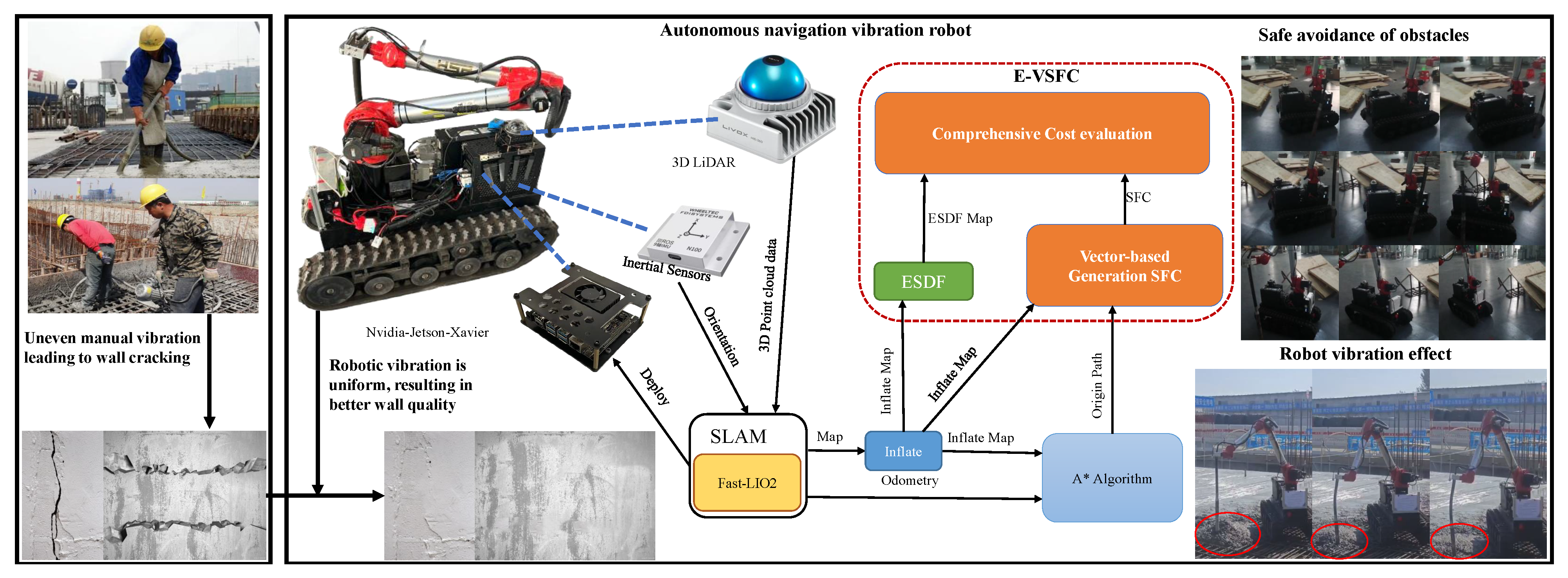
Figure 1.
Diagram illustrating the hardware system framework of the vibration robot. The red circle highlights the research content of this study.
Figure 1.
Diagram illustrating the hardware system framework of the vibration robot. The red circle highlights the research content of this study.
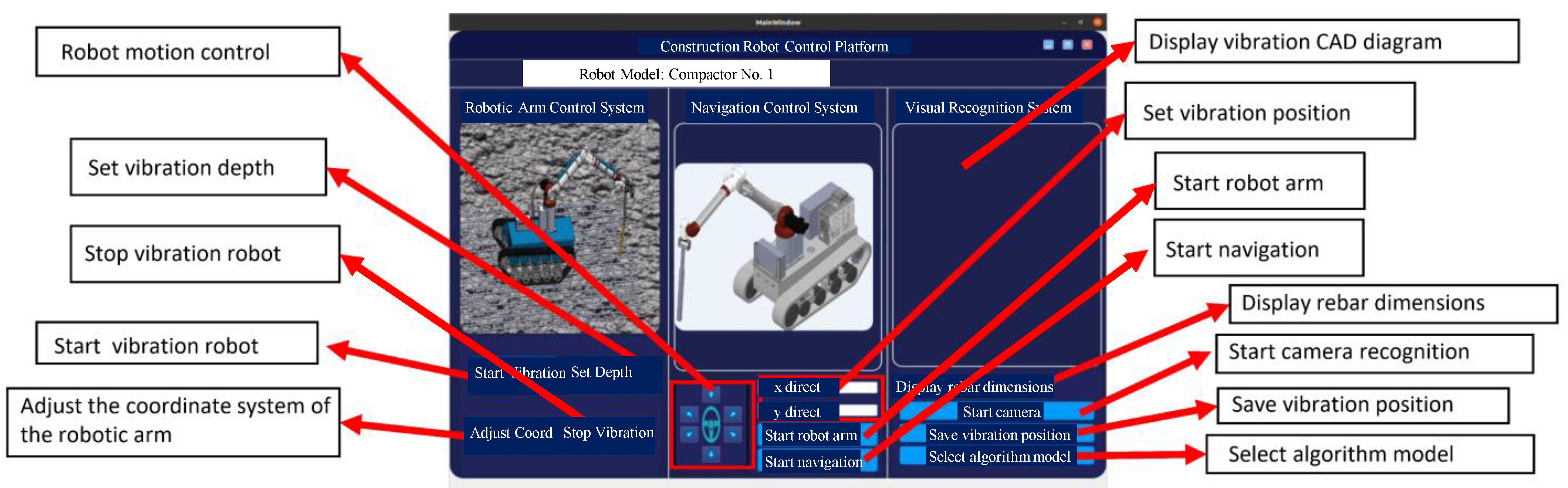
Figure 2.
Explanation of the graphical user interface (GUI) functions for the vibration robot.
Figure 2.
Explanation of the graphical user interface (GUI) functions for the vibration robot.
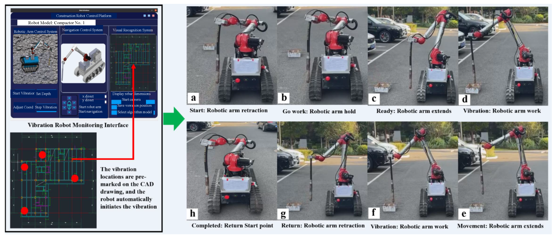
Figure 3.
Process flow diagram of the vibration robot system.
Figure 3.
Process flow diagram of the vibration robot system.
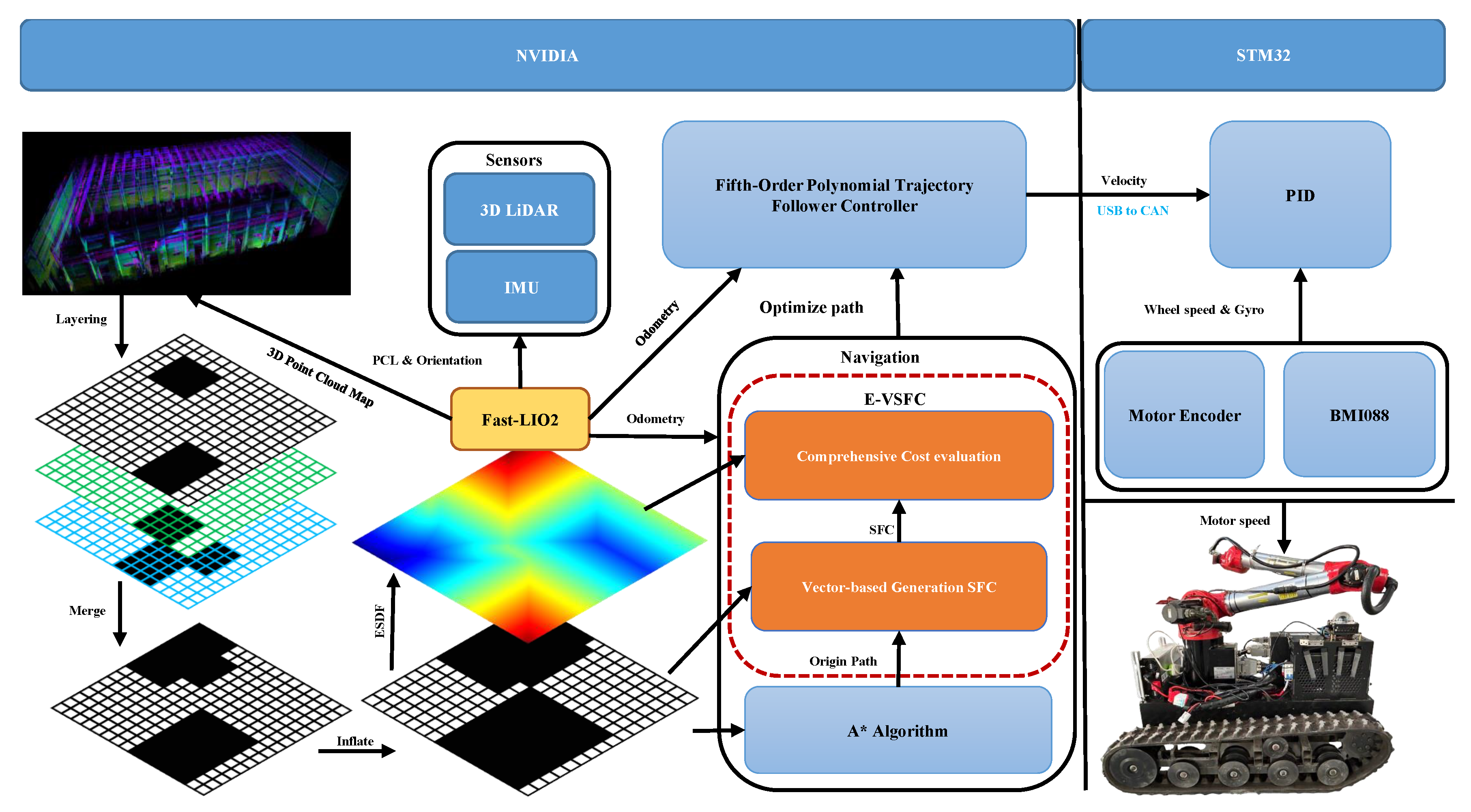
Figure 4.
Research framework diagram of the vibration robot software system.
Figure 4.
Research framework diagram of the vibration robot software system.
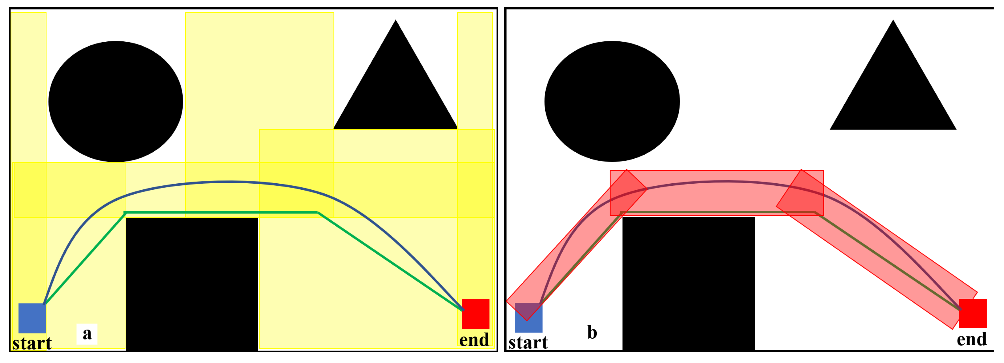
Figure 5.
Safe flight corridor generation diagram. The black sections in the figure represent obstacles. (a) shows the corridor range generated by the traditional method for optimizing the path. (b) shows the corridor range required for the actual optimized path.
Figure 5.
Safe flight corridor generation diagram. The black sections in the figure represent obstacles. (a) shows the corridor range generated by the traditional method for optimizing the path. (b) shows the corridor range required for the actual optimized path.
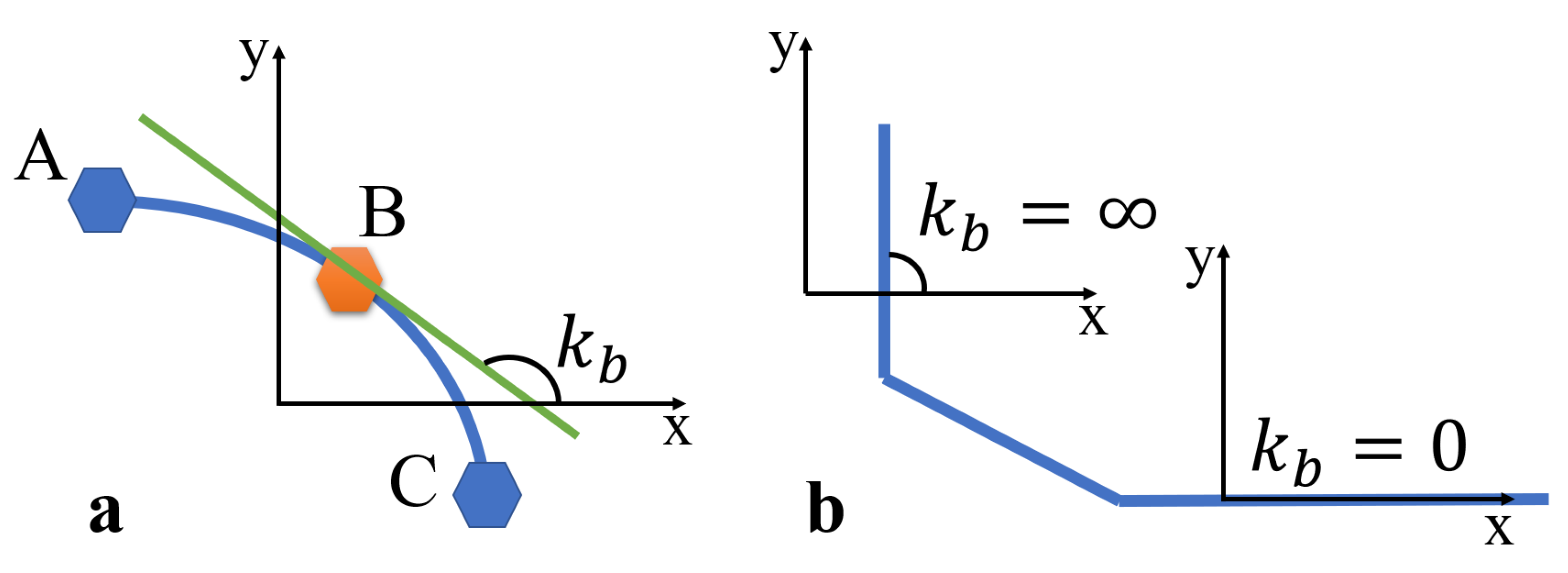
Figure 6.
Derivative method. (a) Under normal conditions, the slope at point B is solved by fitting a curve through points A, B, and C. (b) When points A, B, and C are aligned in a vertical or horizontal line, solving for the slope at point B results in no solution.
Figure 6.
Derivative method. (a) Under normal conditions, the slope at point B is solved by fitting a curve through points A, B, and C. (b) When points A, B, and C are aligned in a vertical or horizontal line, solving for the slope at point B results in no solution.
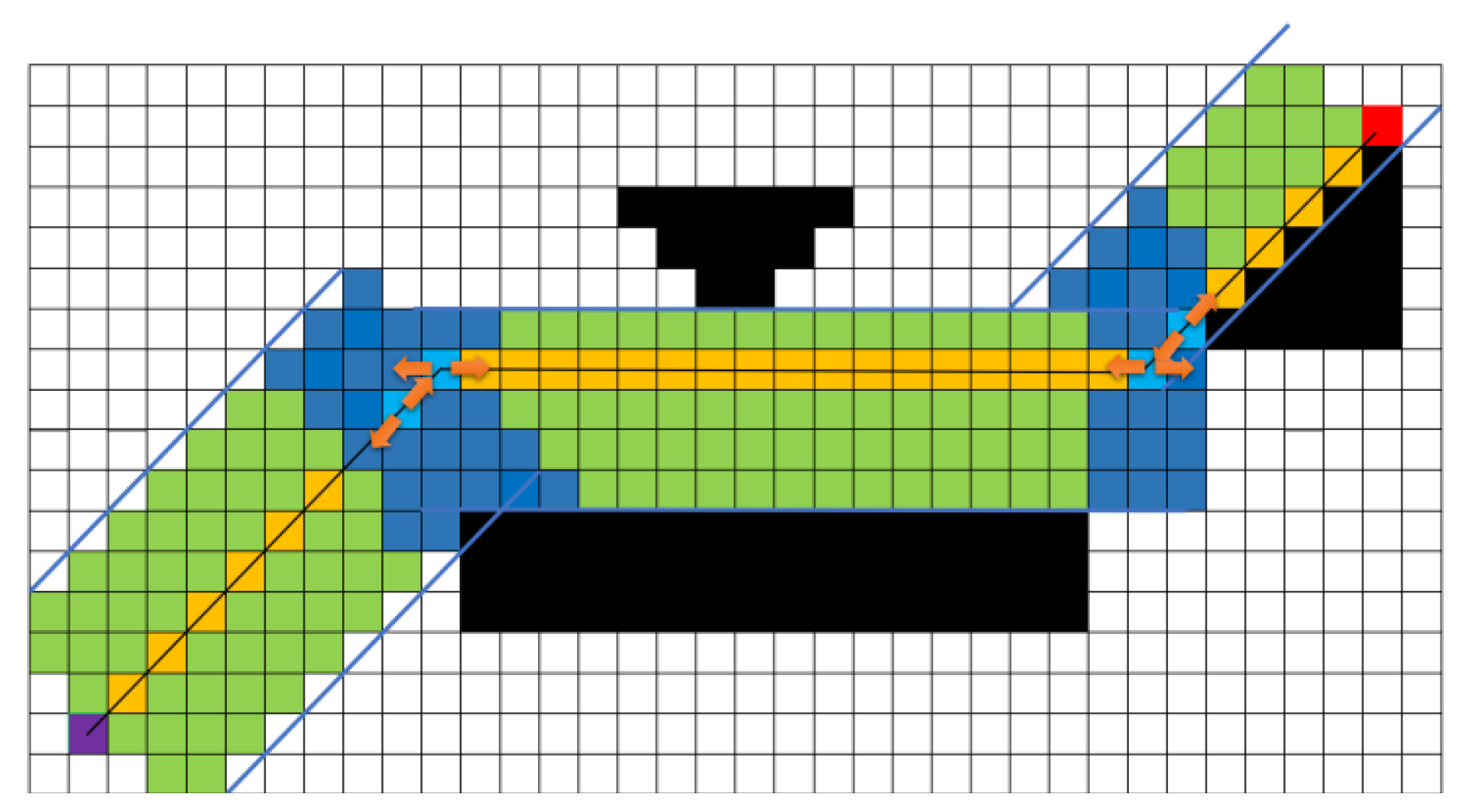
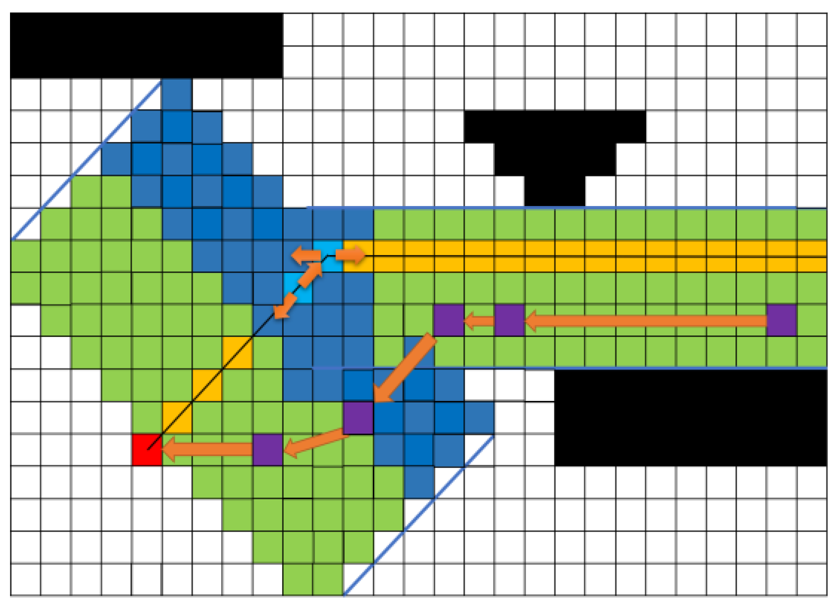
Figure 7.
Vector method. (a) The vector method is used to solve for the normal vector at point B. (b) The difference between solving at point B using the vector method and the conventional method.
Figure 7.
Vector method. (a) The vector method is used to solve for the normal vector at point B. (b) The difference between solving at point B using the vector method and the conventional method.
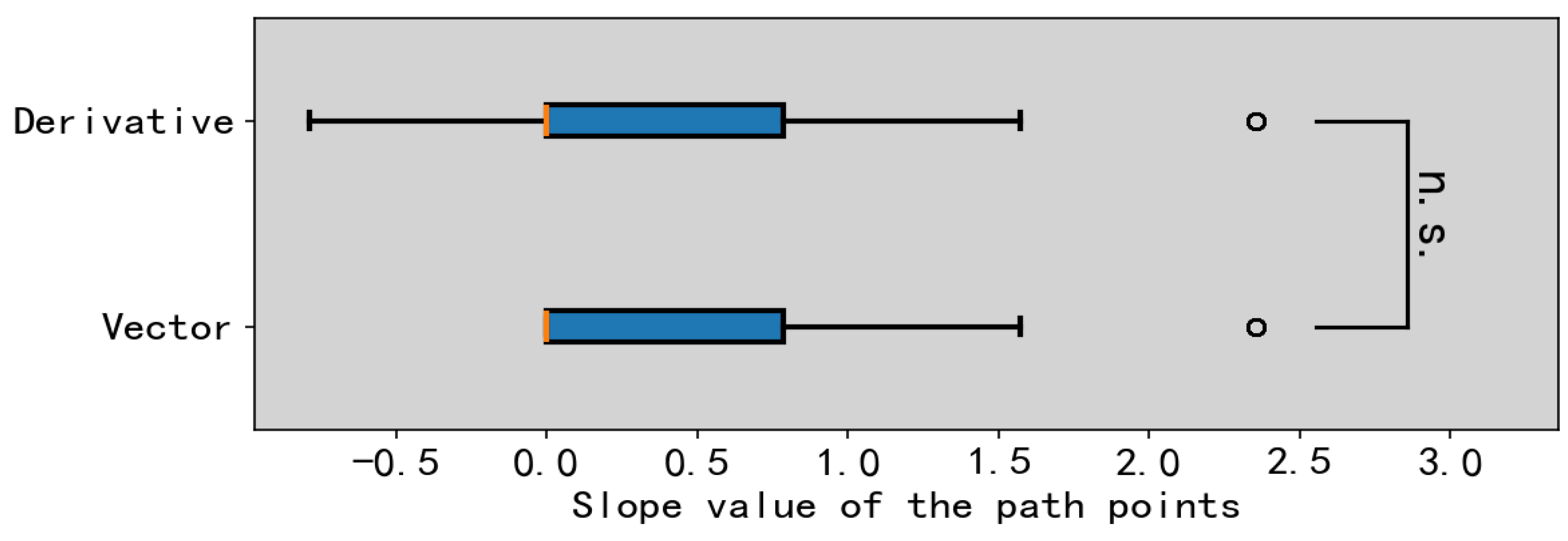
Figure 8.
Data comparison of differences between vector method and derivative method for solving the normal vector slope.
Figure 8.
Data comparison of differences between vector method and derivative method for solving the normal vector slope.
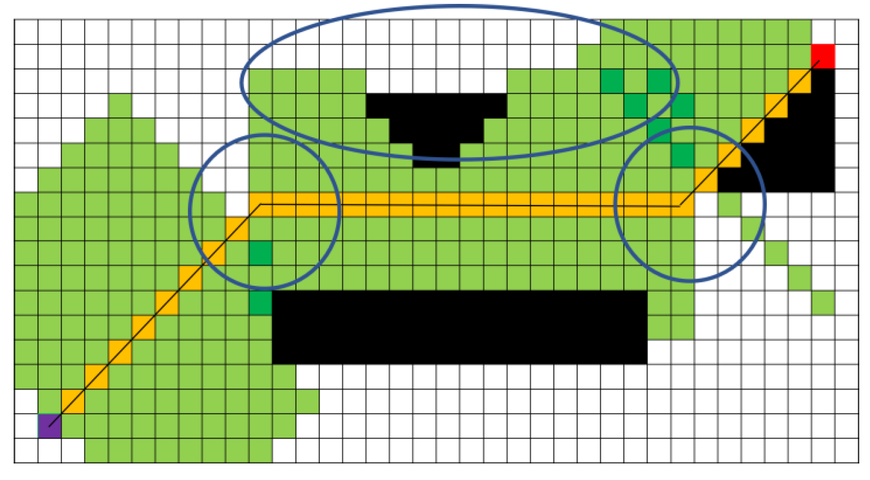
Figure 9.
The corridor generated without pre-expansion.
Figure 9.
The corridor generated without pre-expansion.
Figure 10.
The corridor generated with pre-expansion.
Figure 10.
The corridor generated with pre-expansion.
Figure 11.
Only consider the path optimized by ESDF.
Figure 11.
Only consider the path optimized by ESDF.
Figure 12.
Comprehensive cost assessment.
Figure 12.
Comprehensive cost assessment.
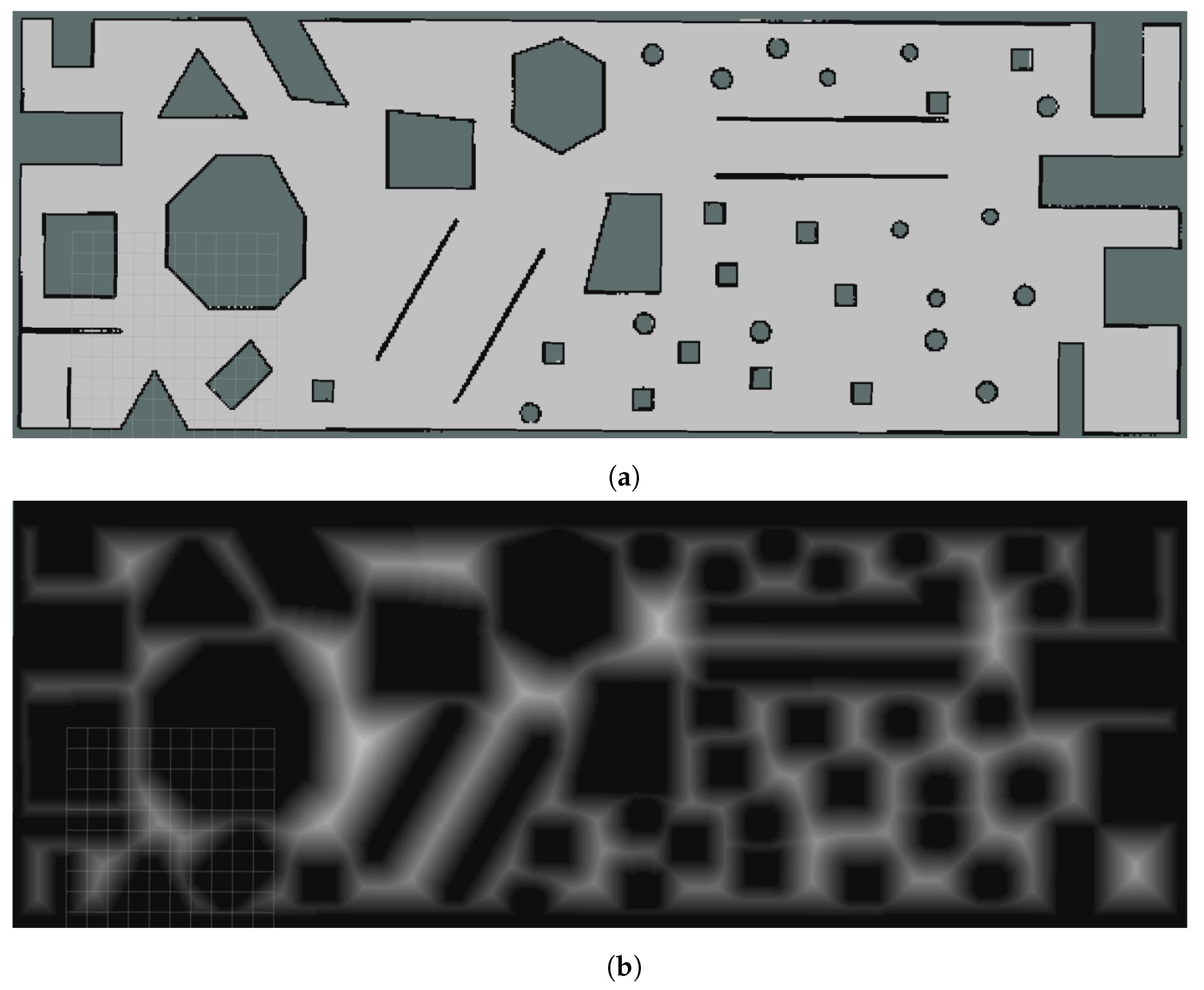
Figure 13.
Randomly generated and ESDF processing maps. (a) Randomly generated maps. (b) ESDF processing of randomly generated maps.
Figure 13.
Randomly generated and ESDF processing maps. (a) Randomly generated maps. (b) ESDF processing of randomly generated maps.
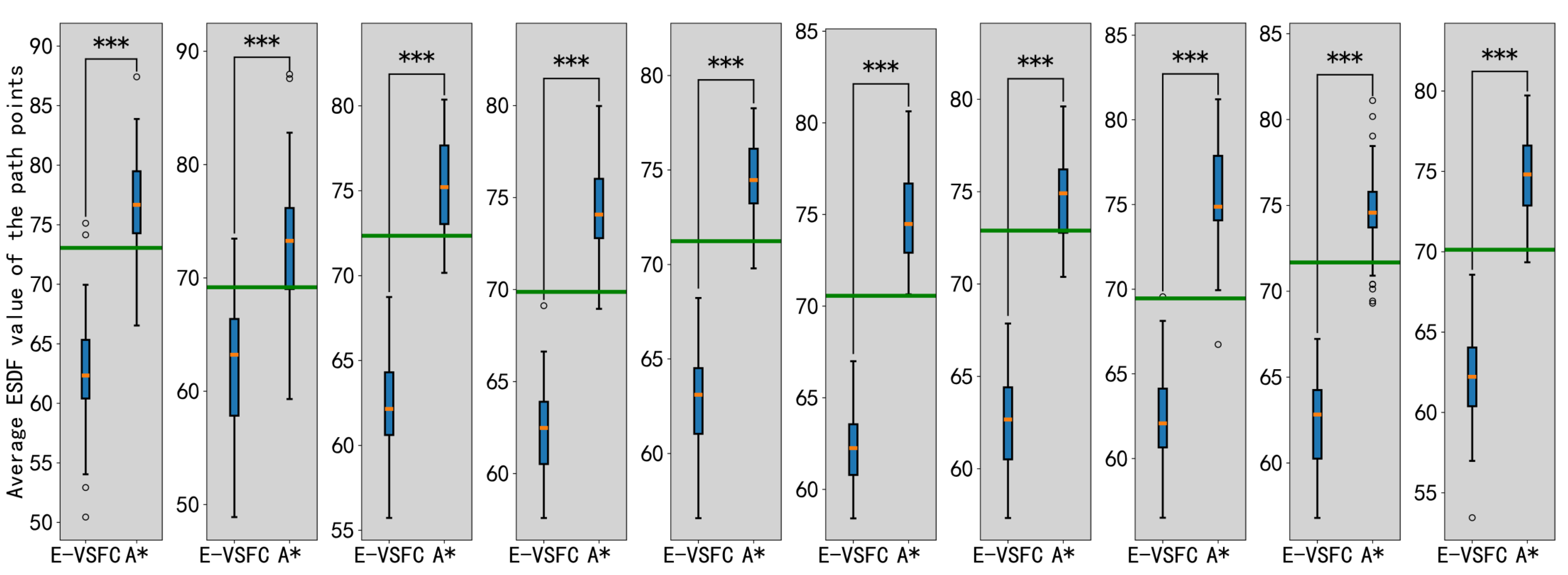
Figure 14.
Significance analysis of the difference in ESDF values between E-VSFC-optimized path and A*-generated paths.
Figure 14.
Significance analysis of the difference in ESDF values between E-VSFC-optimized path and A*-generated paths.
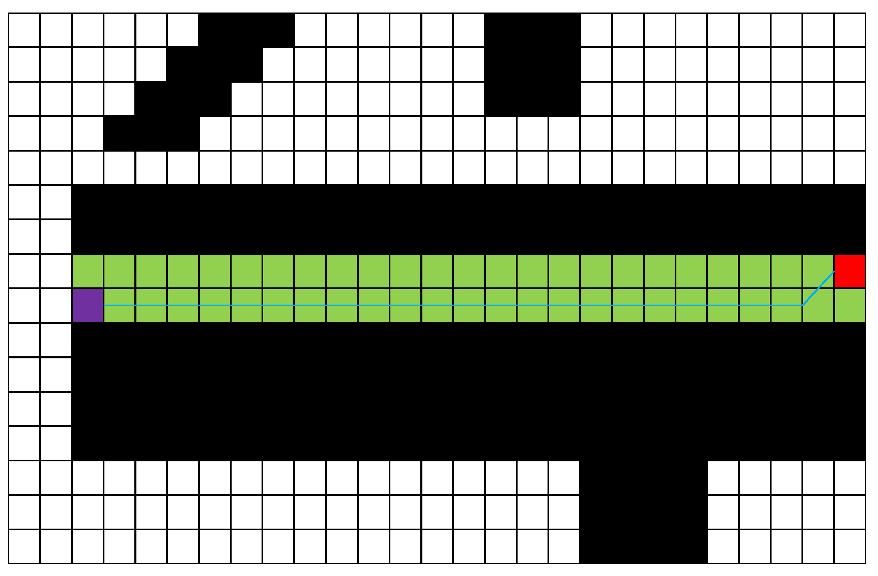
Figure 15.
The situation where the initial path generates a very narrow corridor in densely obstructed areas, resulting in minimal optimization effects.
Figure 15.
The situation where the initial path generates a very narrow corridor in densely obstructed areas, resulting in minimal optimization effects.
Figure 16.
Comparison of E-VSFC-optimized paths and A*-generated paths.
Figure 16.
Comparison of E-VSFC-optimized paths and A*-generated paths.
Figure 17.
Tracked chassis for vibration robots.
Figure 17.
Tracked chassis for vibration robots.
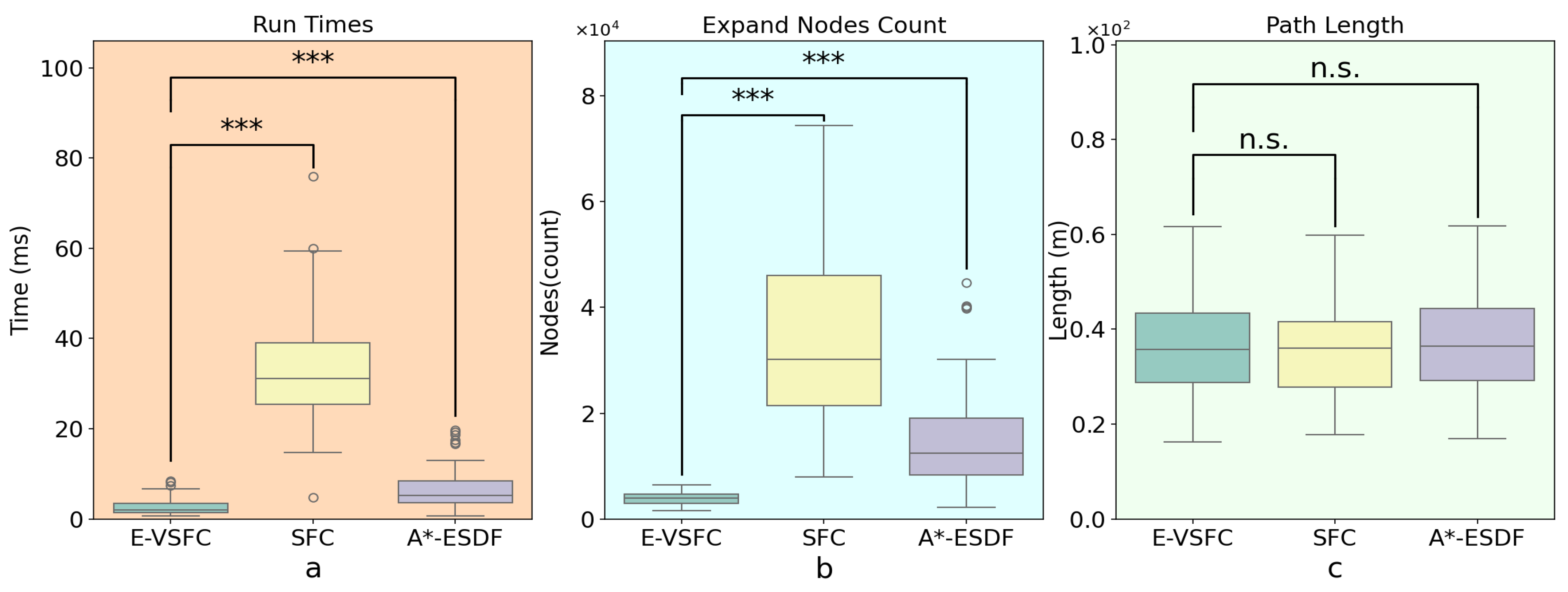
Figure 18.
Comparison of path optimization results for E-VSFC, SFC, and A*-ESDF on simulation maps. (a) Comparison run times (b) Comparison number of expanded nodes (c) Comparison optimized path lengths.
Figure 18.
Comparison of path optimization results for E-VSFC, SFC, and A*-ESDF on simulation maps. (a) Comparison run times (b) Comparison number of expanded nodes (c) Comparison optimized path lengths.
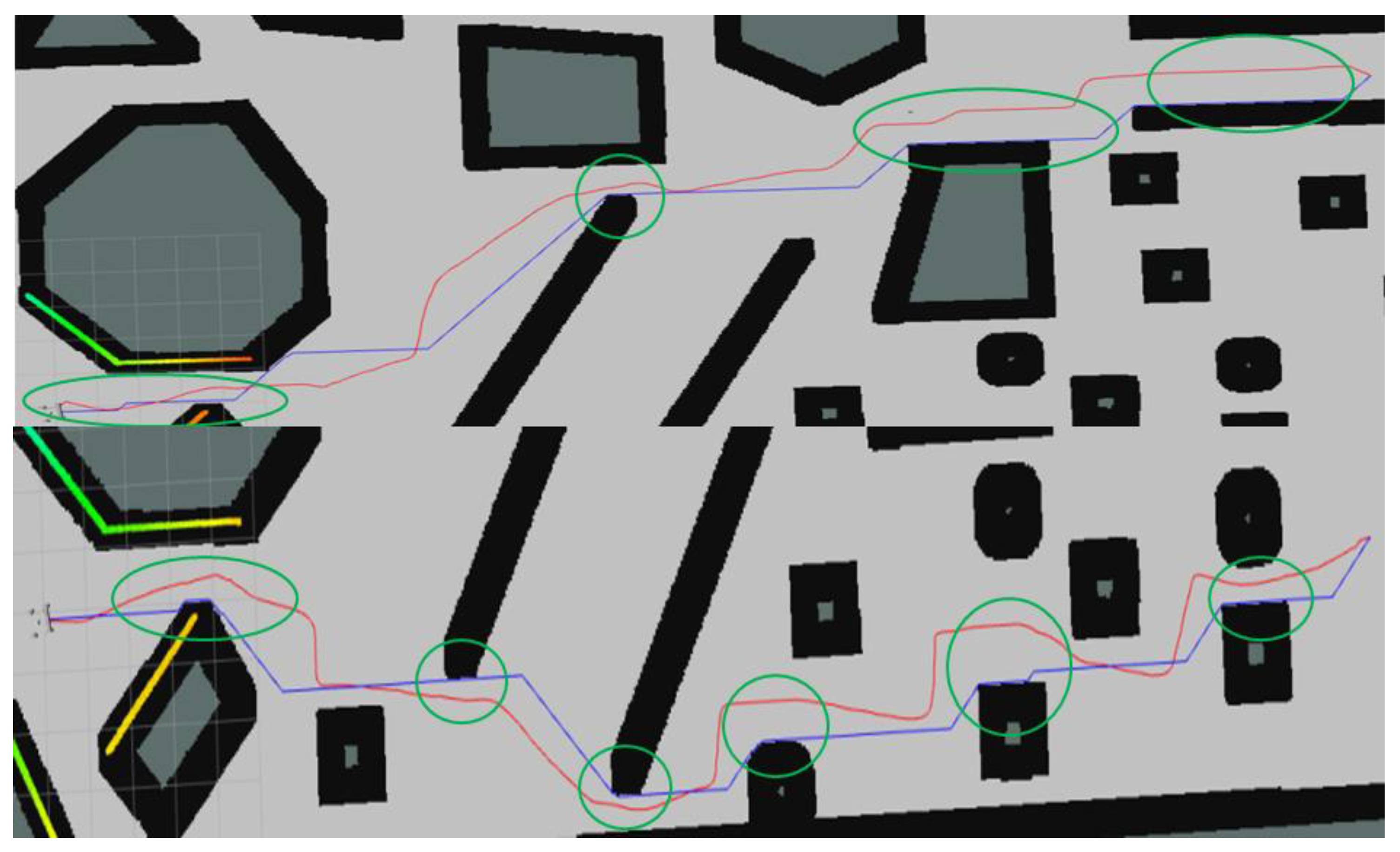
Figure 19.
Red is the E-VSFC path, yellow is the SFC path, blue is the A*-ESDF path, and green is the origin path.
Figure 19.
Red is the E-VSFC path, yellow is the SFC path, blue is the A*-ESDF path, and green is the origin path.
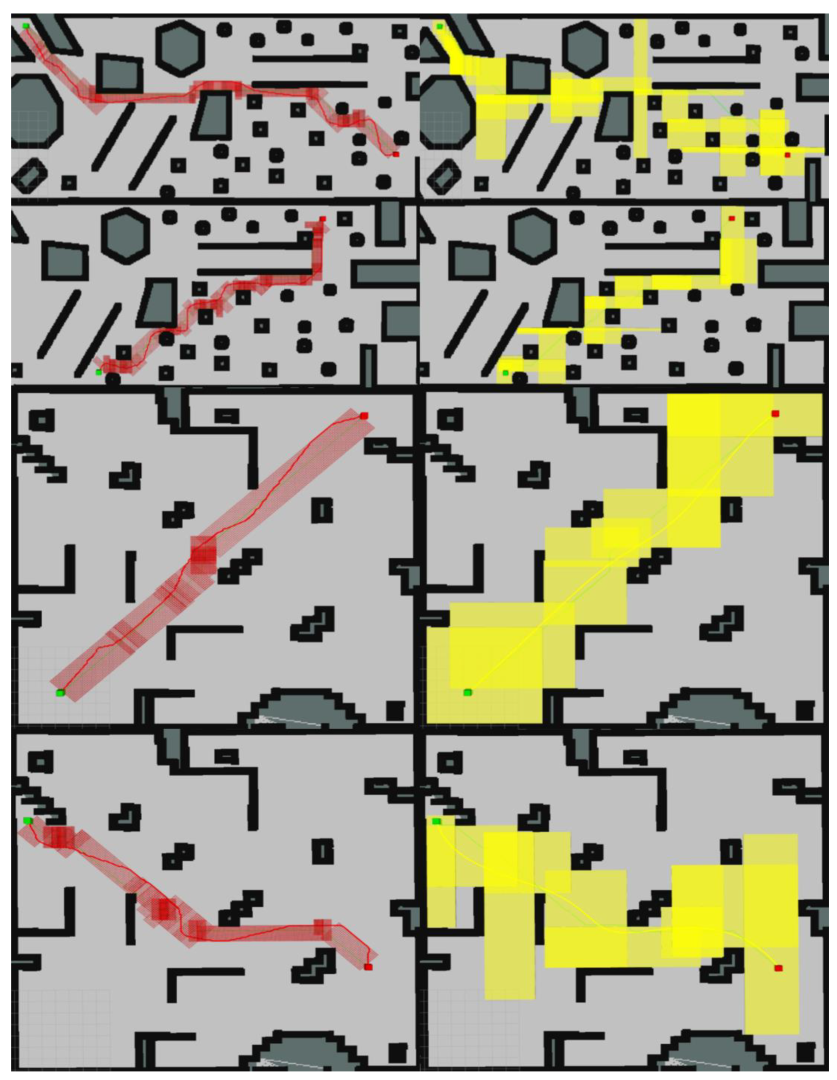
Figure 20.
The red transparent area is the corridor constructed by E-VSFC, while the yellow transparent area is the corridor constructed by SFC. Green is start point, and red is endpoint.
Figure 20.
The red transparent area is the corridor constructed by E-VSFC, while the yellow transparent area is the corridor constructed by SFC. Green is start point, and red is endpoint.
Figure 21.
Mapping of the actual construction environment. (a) CAD drawing of the actual construction environment. (b) SLAM mapping of the actual construction environment.
Figure 21.
Mapping of the actual construction environment. (a) CAD drawing of the actual construction environment. (b) SLAM mapping of the actual construction environment.
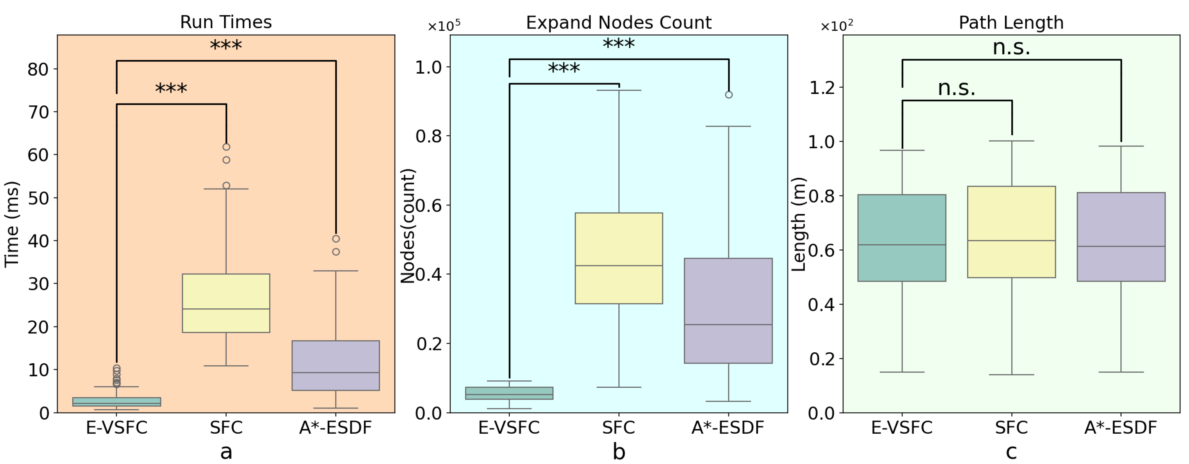
Figure 22.
Comparison of path optimization results for E-VSFC, SFC, and A*-ESDF in the actual construction. (a) Comparison run times (b) Comparison number of expanded nodes (c) Comparison optimized path lengths.
Figure 22.
Comparison of path optimization results for E-VSFC, SFC, and A*-ESDF in the actual construction. (a) Comparison run times (b) Comparison number of expanded nodes (c) Comparison optimized path lengths.
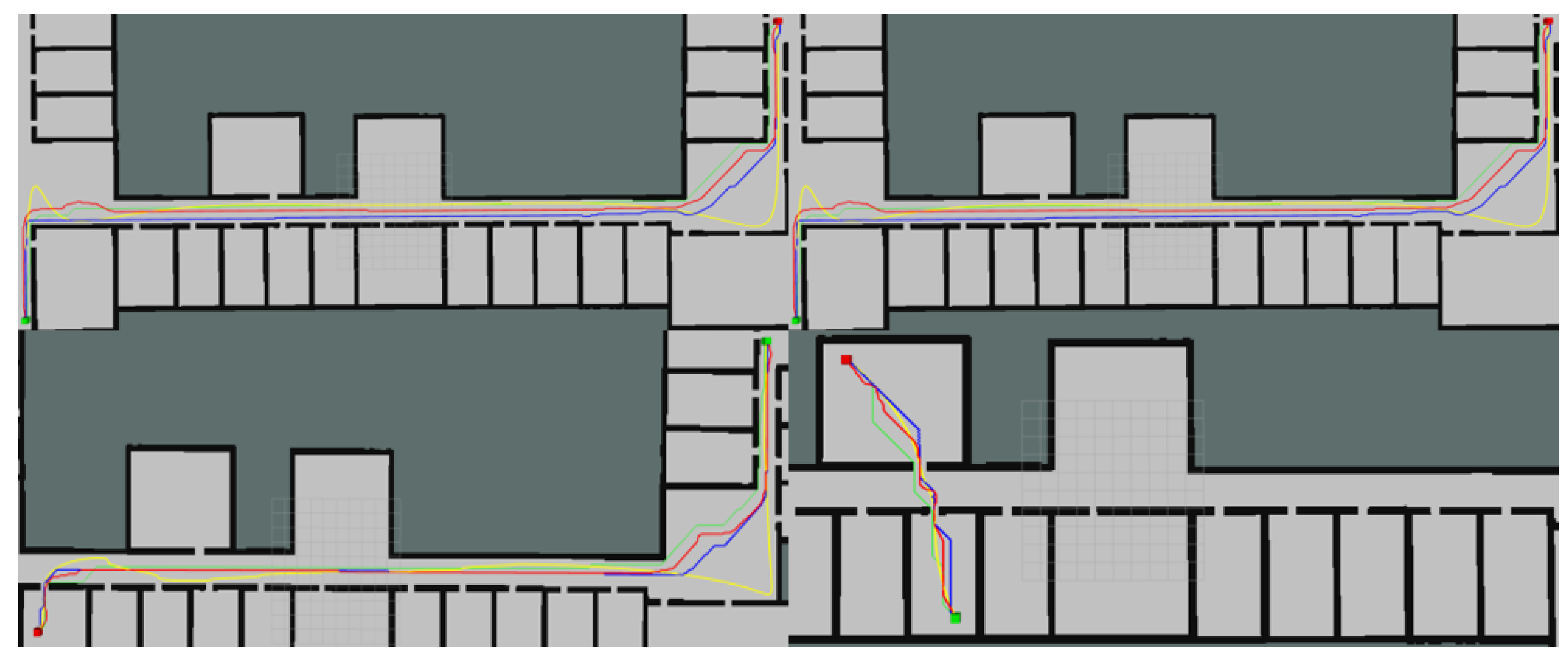
Figure 23.
Red is E-VSFC path, yellow is SFC path, blue is A*-ESDF path, and green is origin path operational data for E-VSFC, SFC, and A*-ESDF in the actual construction site.
Figure 23.
Red is E-VSFC path, yellow is SFC path, blue is A*-ESDF path, and green is origin path operational data for E-VSFC, SFC, and A*-ESDF in the actual construction site.
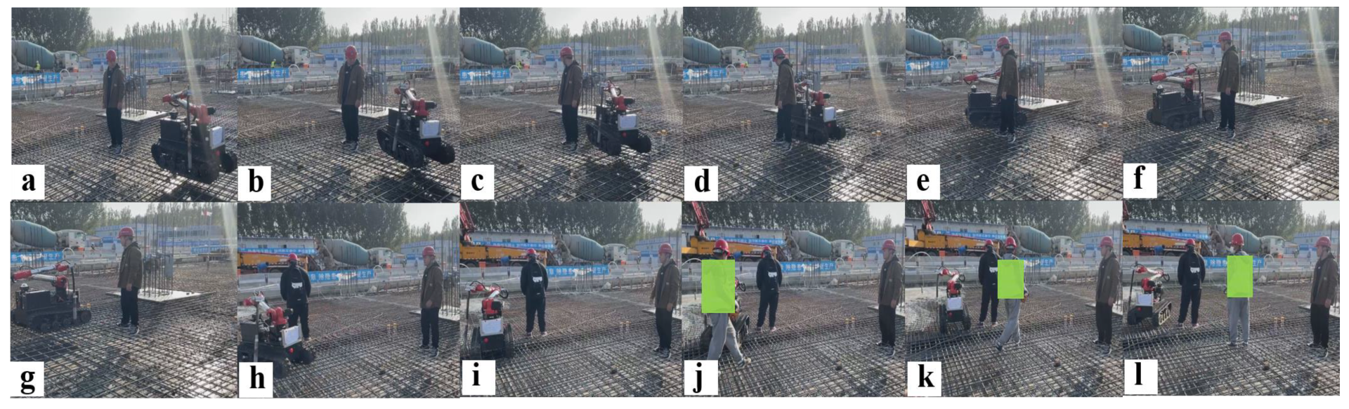
Figure 24.
The site operation of the vibration robot: (a–i) The robot autonomously navigates, avoiding fixed obstacles; (j–l) the robot can autonomously avoid sudden obstacles during its movement.
Figure 24.
The site operation of the vibration robot: (a–i) The robot autonomously navigates, avoiding fixed obstacles; (j–l) the robot can autonomously avoid sudden obstacles during its movement.
Table 1.
Time consumption for path sampling using vector and derivative method.
Table 1.
Time consumption for path sampling using vector and derivative method.
| Path Points | Vector Time (ms) | Derivative Time (ms) |
|---|
| 863 | 0.018 | 1.025 |
| 749 | 0.014 | 0.950 |
| 668 | 0.014 | 0.825 |
| 256 | 0.007 | 0.353 |
| 290 | 0.008 | 0.380 |
| 737 | 0.021 | 1.509 |
| 820 | 0.016 | 1.257 |
| 825 | 0.017 | 1.183 |
Table 2.
Comparison of total path points, total ESDF values, and average ESDF values between A* and E-VSFC algorithms.
Table 2.
Comparison of total path points, total ESDF values, and average ESDF values between A* and E-VSFC algorithms.
| Path Points | Total ESDF | Average ESDF |
|---|
| A* | E-VSFC | A* | E-VSFC | A* | E-VSFC |
|---|
| 498 | 266 | 37,133 | 16,734 | 75 | 63 |
| 283 | 152 | 21,770 | 8223 | 77 | 54 |
| 433 | 245 | 33,194 | 15,565 | 77 | 64 |
| 526 | 274 | 37,954 | 16,989 | 72 | 62 |
| 338 | 182 | 24,054 | 11,054 | 71 | 61 |
| 513 | 271 | 38,653 | 15,407 | 75 | 57 |
| 167 | 101 | 11,319 | 5346 | 68 | 53 |
| 451 | 263 | 34,915 | 16,183 | 77 | 62 |
| 333 | 188 | 24,739 | 11,407 | 74 | 61 |
| 361 | 200 | 27,911 | 13,495 | 77 | 67 |
Table 3.
Main parameters of the chassis.
Table 3.
Main parameters of the chassis.
| Parameter Type | Parameter Value |
|---|
| L | 1.25 m |
| w | 0.7 m |
| 0.4 m |
| 193 kg |
| ±2.0 m/s |
| ±2.0 m/s2 |
| 1.57 rad/s |
Table 4.
Algorithm parameters for E-VSFC, SFC, and A*-ESDF.
Table 4.
Algorithm parameters for E-VSFC, SFC, and A*-ESDF.
| Algorithm | Parameter Type | Parameter Value |
|---|
| | Corridor Width | 2.0 m |
| | | 2.0 |
| E-VSFC | | 1.0 |
| | | 1.0 |
| | | 1.0 |
| | Maximum Speed | ±2.0 m/s |
| | Maximum Acceleration | ±2.0 m/s2 |
| SFC | Edge Distance | 0.4 m |
| | Polynomial Degree | 3 |
| | Number Control Points | 8 |
| A*-ESDF | ESDF Coefficient | 1.0 |
Table 5.
Running data of E-VSFC, SFC, and A-ESDF in random maps, bold indicate the minimum values under the corresponding metrics.
Table 5.
Running data of E-VSFC, SFC, and A-ESDF in random maps, bold indicate the minimum values under the corresponding metrics.
| Run Time (ms) | Expand Nodes | Path Length (m) |
|---|
| E-VSFC | SFC | A*-ESDF | E-VSFC | SFC | A*-ESDF | E-VSFC | SFC | A*-ESDF |
|---|
| 1.04 | 61.23 | 11.12 | 4240 | 28013 | 25807 | 41.28 | 38.6 | 43.7 |
| 6.65 | 50.79 | 12.15 | 4814 | 37594 | 18610 | 40.68 | 38.7 | 40.9 |
| 2.44 | 34.56 | 4.77 | 3407 | 39087 | 12599 | 31.93 | 31.7 | 32.9 |
| 1.59 | 48.85 | 3.09 | 5127 | 53084 | 8542 | 47.52 | 46.5 | 48.5 |
| 1.37 | 33.78 | 4.73 | 4401 | 51637 | 7099 | 39.31 | 39.5 | 40.6 |
| 1.22 | 38.62 | 12.21 | 4939 | 50474 | 26110 | 43.82 | 44.2 | 45.8 |
| 1.55 | 4.74 | 4.74 | 3112 | 7952 | 7952 | 25.54 | 24.7 | 24.7 |
| 1.69 | 18.75 | 2.45 | 2594 | 12777 | 5274 | 26.35 | 26.3 | 26.3 |
| 2.79 | 18.49 | 5.35 | 3172 | 13433 | 12462 | 30.63 | 31.1 | 32.2 |
| 1.30 | 28.52 | 1.50 | 3760 | 29662 | 3735 | 35.56 | 36.1 | 36.3 |
Table 6.
Running data of E-VSFC, SFC, and A-ESDF in actual construction, bold indicate the minimum values under the corresponding metrics.
Table 6.
Running data of E-VSFC, SFC, and A-ESDF in actual construction, bold indicate the minimum values under the corresponding metrics.
| Run time (ms) | Expand Nodes | Path length (m) |
|---|
| E-VSFC | SFC | A*-ESDF | E-VSFC | SFC | A*-ESDF | E-VSFC | SFC | A*-ESDF |
|---|
| 1.4 | 23.40 | 4.1 | 4392 | 31318 | 13475 | 58.3 | 62.4 | 58.6 |
| 3.3 | 28.88 | 21.3 | 6367 | 52508 | 54811 | 80.1 | 82.4 | 80.8 |
| 2.2 | 20.88 | 10.6 | 8818 | 39697 | 30704 | 79.1 | 84.5 | 78.8 |
| 1.1 | 14.61 | 2.8 | 4446 | 27728 | 9217 | 44.4 | 46.1 | 44.2 |
| 5.6 | 52.05 | 18.3 | 6895 | 70649 | 51436 | 71.2 | 74.8 | 70.8 |
| 2.2 | 29.53 | 15.3 | 7763 | 64298 | 42951 | 94.7 | 97.7 | 95.3 |
| 3.2 | 26.08 | 20.9 | 6796 | 61511 | 52408 | 82.4 | 86.1 | 82.5 |
| 1.2 | 33.85 | 17.2 | 4503 | 58796 | 44839 | 57.2 | 58.2 | 57.7 |
| 1.3 | 24.05 | 8.1 | 4790 | 42558 | 23042 | 52.9 | 52.6 | 52.3 |
| 5.0 | 33.03 | 22.1 | 7297 | 53391 | 61409 | 87.5 | 89.7 | 88.2 |
Table 7.
Statistics of planning results in the construction site.
Table 7.
Statistics of planning results in the construction site.
| | Stop Radius/m | Finish Task | Run Time/s | Collisions | Path Length/m |
|---|
| Static | Move | A* | E-VSFC | A* | E-VSFC | A* | E-VSFC | A* | E-VSFC | A* | E-VSFC |
|---|
| 0 | 0 | 0.31 | 0.13 | Yes | Yes | 177 | 193 | 0 | 0 | 87.8 | 95.6 |
| 6 | 0 | 0.32 | 0.12 | Yes | Yes | 371 | 267 | 2 | 0 | 91.3 | 103.2 |
| 6 | 0 | 0.25 | 0.14 | Yes | Yes | 353 | 274 | 1 | 0 | 99.5 | 110.7 |
| 7 | 1 | 0.33 | 0.09 | Yes | Yes | 427 | 358 | 1 | 0 | 101 | 119.8 |
| 7 | 2 | - | 0.13 | No | Yes | - | 401 | 3 | 0 | - | 137.4 |
| 8 | 0 | 0.27 | 0.11 | Yes | Yes | 239 | 283 | 1 | 0 | 101 | 107.8 |
| 8 | 1 | 0.23 | 0.14 | Yes | Yes | 314 | 287 | 4 | 0 | 94.6 | 102.9 |
| 8 | 2 | - | 0.13 | No | Yes | - | 361 | 3 | 0 | - | 97.2 |
| 8 | 3 | - | 0.15 | No | Yes | - | 371 | 2 | 0 | - | 89.3 |
| 8 | 4 | - | 0.13 | No | Yes | - | 324 | 5 | 0 | - | 107.3 |


 ,
, 


