Abstract
The performance of passive target localization is affected by the positions of unmanned aerial vehicles (UAVs) at a large scale. In this paper, to improve resource utilization efficiency and localization accuracy, the node selection problem and the path optimization problem are jointly investigated. Firstly, the target passive localization model is established and the Chan-based time difference of arrival (TDOA) localization method is introduced. Then, the Cramer–Rao lower bound (CRLB) for Chan-TDOA localization is derived, and the problems of node selection and path optimization are formulated. Secondly, a CRLB-based node selection method is proposed to properly divide the UAVs into several groups, localizing different targets, and a CRLB-based path optimization method is proposed to search for the optimal UAV position configuration at each time step. The proposed path optimization method also effectively handles no-fly-zone (NFZ) constraints, ensuring operational safety while maintaining optimal target tracking performance. Also, to improve the efficiency of path optimization, particle swarm algorithm (PSO) is applied to accelerate the searching process. Finally, numerical simulations are performed to verify the validity and effectiveness of the proposed methods in this paper.
1. Introduction
Unmanned Aerial Vehicle swarms (UAVs) have indeed become integral components of modern military operations, particularly in real-time aerial reconnaissance, surveillance, and various tactical applications. The versatility and technological capabilities provide numerous advantages, and their adoption has significantly transformed the landscape of modern warfare [1,2]. Recently, UAVs have garnered significant attention for their enhanced capabilities in complex missions such as target tracking, localization, and detection [3,4,5]. The distributed nature of UAVs provides robust and flexible operations, particularly in challenging tactical environments.
Generally, UAVs can be burdened by active systems or passive systems to fulfill their tasks. For active localization systems, the locator (such as a radar) actively emits signals to detect and determine the position of targets. While this can provide real-time tracking and high precision, it exposes the location of the locator itself to enemy detection. This makes active localization vulnerable in hostile environments, especially in situations where stealth and secrecy are crucial. Additionally, active localization systems tend to require higher energy consumption and more complex infrastructure, which can be a logistical challenge [6,7]. On the other hand, a passive localization system does not involve emitting signals. Instead, it works by detecting and analyzing the electromagnetic waves emitted by the target’s own electronic devices. The key advantage is that it does not disclose the location of the system receiving the signals, making it inherently more stealthy and harder to detect [8,9,10]. In this case, UAVs’ passive localization technology offers significant strategic advantages in situations where stealth, resource efficiency, and survivability are crucial. Its ability to detect targets without emitting signals makes it a powerful tool in modern military operations [11,12].
1.1. Overview
For multi-target passive localization via UAVs, node selection and path optimization are crucial to enhance the accuracy and efficiency of target localization, since through node selection, the UAVs could be properly divided into several groups to locate different targets, and through path optimization, the UAVs could achieve proper positions at each frame, obtaining appropriate observation angles and high-quality measurements that help realize high localization accuracy. Therefore, dynamic node selection and path optimization could help ensure that UAVs are optimally positioned to minimize errors in localization, improving the ability of the UAVs in locating a target.
From the perspective of node selection for the UAVs, node selection could be implemented via classic greedy algorithms to construct minimum spanning trees (MSTs) to select a set of UAVs that minimizes the total communication or distance between them [13,14]. Task scheduling also needs to select a set of UAV nodes to optimize task scheduling and load balancing in distributed UAV systems [15,16].
More recently, reinforcement learning (RL) approaches have shown promising results in UAV path planning and navigation tasks. Deep reinforcement learning (DRL) methods, particularly algorithms like deep Q-networks (DQNs) and proximal policy optimization (PPO), have been successfully applied to autonomous navigation in complex environments [17]. These methods enable UAVs to learn optimal navigation policies through interactions with the environment without requiring complete prior knowledge of the operational space. Particularly noteworthy is the development of cross-platform deep reinforcement learning approaches for autonomous navigation without global localizing information [18], which have demonstrated remarkable adaptability across different scenarios and vehicle platforms. Such end-to-end learning approaches that combine local sensor information with learned policies have significantly advanced the field of autonomous navigation [19].
Additionally, ant colony optimization (ACO) could be deployed for node selection to determine optimal routes for the communication relay of coverage tasks, ensuring minimal energy expenditure while still fulfilling the mission’s objectives [20,21], and for a UAV network, the central leader node selection is essential for coordinating tasks and managing communications [22].
From the perspective of path optimization for UAVs, the heuristic-based A* algorithm is used for path optimization to efficiently find the shortest path [23]. The genetic algorithm (GA) is introduced to cooperative path planning for UAVs. It uses a population of potential solutions (paths), which evolve over generations according to a fitness function, and the algorithm incorporates crossovers with mutation operations to explore the solution space while the fitness function guides the search toward optimal or near-optimal paths that avoid collisions and optimize mission objectives [24]. The differential evolution (DE) algorithm is well suited for UAV path optimization because of its ability to efficiently search high-dimensional spaces while minimizing time and energy consumption [25]. The bat algorithm adapts well to dynamic environments and is used to optimize UAV trajectories in the presence of changing obstacles or mission requirements [26].
A projection algorithm has been deployed to improve the localization accuracy of UAVs, and the algorithm guides UAVs toward way points that are closer to the target. This approach reduces the computational burden associated with numerical searches by projecting UAVs onto more promising paths based on predictive models, thus improving the efficiency and effectiveness of the path optimization process [27]. Although this algorithm considers the application of target passive localization, it only considers one target.
Concerning existing works, it can be seen that in most works, node selection and path optimization are separately investigated, which restricts performance improvements in localization accuracy for multi-targets. Also, node selection methods in existing works are mainly concerned with task scheduling, resources distribution, and communication link construction, and the path optimization methods in the existing works are mainly concerned with the shortest path searching and obstacle avoidance operations with less resource consumption, which ignore the application multi-target passive localization. Additionally, existing path optimization methods rarely consider the integration of no-fly-zone constraints with localization performance optimization, which is crucial for practical UAV operations in restricted airspace. Furthermore, while reinforcement learning approaches have shown promising results in UAV navigation, they often require extensive training data and computational resources, and their performance in multi-target passive localization applications remains largely unexplored. The existing deep learning models for autonomous navigation typically focus on single-platform scenarios and may not effectively accommodate the complex requirements of coordinated UAVs operations for passive localization.
1.2. Original Contributions
Obviously, works that focus on multi-target passive localization while jointly considering the node selection and the path optimization are rare, and these are indeed the main topics of this paper. In this paper, we jointly consider the problem of node scheduling and path optimization, and we propose a CRLB-based node selection method and a CRLB-based path optimization method to improve localization accuracies. The original contributions of this paper are as follows:
(1) We propose a novel joint optimization framework that unifies node selection and path optimization for multi-target passive localization. Unlike existing methods that handle these problems separately, our integrated approach simultaneously optimizes resource allocation and path planning, achieving superior performance in both resource utilization and localization accuracy.
(2) We develop a CRLB-based node selection method that effectively partitions UAVs into optimal groups for different target localization. This method uniquely considers the theoretical lower bound of estimation errors to guide grouping decisions, leading to improved resource efficiency and localization performance.
(3) We design a CRLB-based path optimization method that dynamically determines optimal UAVs positions by minimizing the theoretical estimation error bound. This approach enables more accurate target localization performance compared to traditional fixed-formation methods.
(4) We implement the PSO algorithm for UAV path optimization. This implementation significantly improves computational efficiency while maintaining solution quality compared to several existing optimization methods.
1.3. Organization
The main contents of this paper are shown as follows. The problems of node selection and path optimization are formulated in Section 2. The algorithm of the node selection based on CRLB is given in Section 3, and the algorithm of the path optimization based on CRLB is given in Section 4. Numerical simulations are given in Section 5. This paper is concluded in Section 6.
2. Problem Formulation
In this section, we present a comprehensive formulation of the multi-target passive localization problem using UAVs based on the Chan-TDOA method. First, we establish the fundamental Chan-TDOA localization model. Then, we derive the CRLB for measurement errors in the Chan-TDOA model to evaluate the theoretical lower bound of the localization performance. Finally, we formulate two key optimization problems: the node selection problem for optimal UAVs grouping and the path optimization problem for determining optimal UAVs positions, which together form a complete framework for multi-target passive localization via UAVs. The mathematical models and theoretical analyses presented in this section serve as the foundation for the algorithms developed in subsequent sections.
2.1. Target Localization Model Based on the Chan-TDOA Algorithm
In sight of the fact that target localization is designed to determine target positions based on measurements, we first establish the fundamental TDOA model. Consider a two-dimensional passive localization scenario with multiple UAVs and targets, as shown in Figure 1.
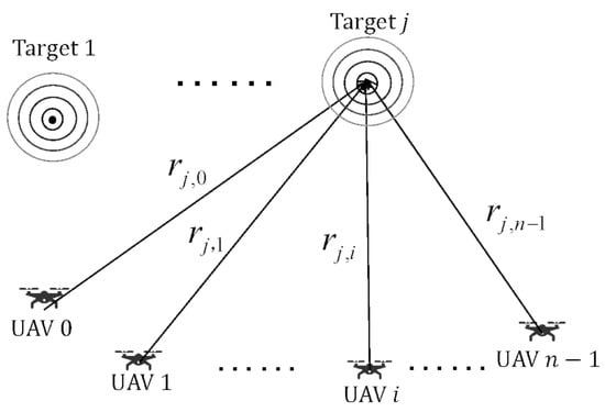
Figure 1.
Geometric schematic of the TDOA localization model. The distance between target j and each UAV is denoted as , where UAV 0 serves as the reference node (or master UAV), and UAV i () represents other nodes in the swarm. The concentric circles around the target indicate the signal propagation.
Assume that there are m stationary targets, and the jth target has coordinates , where . A swarm of n UAVs equipped with passive radars is deployed, and their coordinates are given by , where . Without loss of generality, UAV 0 is selected as the reference node (or master UAV).
The distance between the ith UAV and jth target can be expressed as
For TDOA measurements, let represent the time taken for the signal from target j to reach UAV i. The time difference of arrival between UAV i and the master UAV (UAV 0) is denoted as , where the subscript triplet has the following meaning: The first subscript j indicates the target being localized, the second subscript i represents the measuring UAV, and the third subscript 0 refers to the master UAV (UAV 0). Thus, represents the time difference between when UAV i and UAV 0 receive the signal from target j, which can be written as
where c is the propagation speed of electromagnetic waves.
In practical applications, the measured TDOA value inevitably contains measurement errors:
where represents the measured time difference between UAV i and UAV 0 for target j, is the true time difference, and denotes the time difference error, and it is typically modeled as zero-mean Gaussian noise:
where is the variance of the TDOA measurement for target j, with and being the TDOA measurement variances in UAV i and UAV 0 respectively.
Several factors contribute to the TDOA measurement errors. The internal electronic noise in the radar receiver affects TDOA measurement precision. Signal reflection and refraction during propagation can introduce additional errors. Variations in atmospheric conditions, such as temperature and humidity, impact the propagation speed. The radar’s time resolution also imposes limitations on measurement capabilities. Also, the standard deviation of the TDOA time measurement between UAV i and target j exhibits dependencies on their separation distance:
where and are system parameters determined by the radar characteristics and propagation environment. The parameter is typically close to , reflecting the relationship between signal power attenuation and distance.
For target localization in two dimensions, at least three UAVs are required to obtain sufficient TDOA measurements. When the number of UAVs , the TDOA measurement equations can be used to construct a nonlinear system as follows:
To accelerate the calculation process of nonlinear equations, the Chan algorithm is introduced in this paper to provide an efficient closed-form solution through linearization and two-step weighted least squares estimation. The Chan algorithm is a non-recursive solver for systems of hyperbolic equations that can transform an initially nonlinear system into a linear one. Under the assumption that the TDOA measurement errors follow an ideal Gaussian distribution, the Chan-TDOA localization algorithm can provide high localization accuracies with reduced computational complexity.
For target localization in two dimensions with multiple UAVs (), the Chan-TDOA algorithm provides an efficient closed-form solution through linearization and two-step weighted least squares (WLS) estimation. The algorithm first transforms the nonlinear TDOA equations into linear forms through algebraic manipulation. Then, it employs a two-step WLS estimation process to obtain the target location estimate, with the first step providing an initial solution and the second step refining the estimate. The detailed mathematical derivations of the algorithm are presented in Appendix A. The overall flow of the algorithm is illustrated in Figure 2.
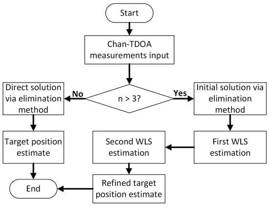
Figure 2.
Flow chart of the Chan-TDOA algorithm.
2.2. CRLB Derivation for TDOA Measurement Errors in the Chan-TDOA Model
The CRLB is an important metric for evaluating parameter estimation performances, representing the smallest possible variance achieved via an unbiased estimator. It is commonly used as a benchmark for comparing the performance of unbiased estimators.
In the context of the Chan-TDOA passive target localization problem discussed in this paper, the observation data of the localization system consists of the TDOA measurements between each UAV and the target. Let the measured TDOA values be denoted as , with the true values given by
where represents the difference in the times at which the signal was received by the ith UAV and the master base station. The measurement is given by
The TDOA measurement error follows a normal distribution , where is the covariance matrix of the TDOA measurements, as given in (A13). The probability density function of the TDOA measurements can be expressed as
The likelihood function calculated from this density function is as follows:
Taking the second partial derivatives of (10) with respect to the position’s coordinate parameters, we have
Then, the Fisher information matrix for the localization parameters can be denoted as
Thus, the CRLB matrix for target position estimations could be obtained by taking the inverse of the Fisher information matrix
2.3. Optimization Problem Formation
In this paper, we formulate two optimization problems for multi-target passive localization via UAVs: the node selection problem and the path optimization problem.
For a swarm of n UAVs and m targets, the node selection problem aims to optimally divide the n UAVs into m groups to minimize the average trace of the derived CRLB for each group’s UAVs localization results at this moment:
where represents the coordinate matrix of all UAVs assigned to target j, and is the trace of the CRLB matrix of the localization for the jth target at the current time step.
For each group of UAVs, the path optimization problem aims to determine the optimal position for each UAV at the next time step to minimize the trace of the derived CRLB, while satisfying the dynamic constraints for the UAV constraints:
where represents the coordinate matrix of all UAVs assigned to target j at the next time step, and is the prediction trace of the CRLB matrix of the localization result for the target j at the next time step.
In the following sections, we will introduce the detailed process of the proposed CRLB-based node selection method and the proposed CRLB-based path optimization method. Then, to accelerate the searching process for the optimal UAV positions, the PSO algorithm is introduced and applied to solve the path optimization problem.
3. CRLB-Based Node Selection Method
In this section, a CRLB-based node selection method is proposed to optimally divide UAVs into groups for localizing different targets, improving localization accuracies. Firstly, we describe the node selection problem and give the constraints of the problem. Then, the optimization model is formulated based on the derived CRLB, and the exhaustive method is deployed to minimize the average CRLB trace and obtain the optimal grouping scheme.
3.1. Problem Description
Consider a surveillance scenario with m stationary targets in a two-dimensional plane. n UAVs equipped with passive radars need to be divided properly into several groups for multi-target localization, and the number of UAVs of each groups for the jth target is . The random assignment of UAVs may lead to suboptimal resource utilization and degraded localization accuracy. Therefore, we develop a systematic method for UAV grouping that ensures optimal performance.
3.2. Constraint Analysis
Since the Chan-TDOA method needs at least 3 UAVs to locate a target in a two-dimensional plane. Thus, the number of UAVs of each group should be more than 3. That is,
3.3. Node Selection Optimization Model
The objective of the node selection problem is to minimize the average CRLB trace across all targets, and the mathematical model can be denoted as follows
where represents the set of UAVs assigned to target j, and denotes the trace of the CRLB matrix for target j at the current time step.
3.4. Node Selection Algorithm Design
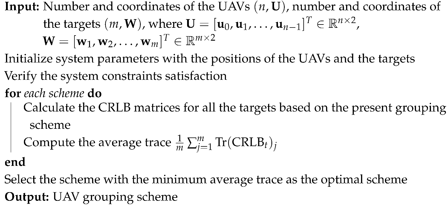
The CRLB-based node selection algorithm provides a systematic approach for optimally grouping UAVs to locate different targets while minimizing localization errors. The algorithm employs a two-stage exhaustive search method: Firstly, it enumerates all possible combinations to partition n UAVs into m groups, where each group must contain at least 3 UAVs () to ensure effective target localization. For each configuration in this solution space, the algorithm computes the CRLB matrices for all targets and calculates their average trace as a metric of localization accuracy, selecting the one that minimizes this metric as the globally optimal solution. The detailed implementation of the node selection method is presented in Algorithm 1.
| Algorithm 1: CRLB-based node selection algorithm |
 |
4. CRLB-Based Path Optimization Method
In this section, we presents a CRLB-based path optimization method to dynamically adjust the UAVs to the optimal positions, enhancing the target localization accuracy. For the sake of a clear presentation in this section, we consider path optimization for a group of UAVs localizing a certain target after node selection; thus, the UAVs have been optimally grouped for each target. In this case, for the convenience of description, target index j is omitted in the following derivations.
4.1. Problem Description
Consider a group of UAVs localizing a target at the current time t. The path planning updates are governed by the optimization time interval . For the convenience of description, it is assumed that each UAV maintains a constant flight speed v during the path planning process. The variables that need to be optimized are the deflection angles of the UAVs, which represent the angles between the heading direction of the UAVs and the positive x-axis (measured counterclockwise), and once the deflection angles are optimized, the positions of the UAVs at time are determined. Thus, optimizing the deflection angles of the UAVs equals optimizing the positions of the UAVs. We assume that the positions of the UAVs at time t are , which can be structured as
where denotes the two-dimensional coordinates of the ith UAV at time t, and represents the total number of the UAVs in the group.
4.2. Constraint Analysis
To ensure the physical feasibility of the UAVs’ movements, we consider four fundamental constraints:
(1) The turning radius constraint: Due to the mechanical limitations of UAVs, the actual turning radius must be greater than the minimum allowable turning radius (which is determined by the system parameters of the UAV). The minimum allowable turning radius is as follows:
The turning radius can be determined by the UAV’s movement during the path planning time interval . We assume that within the time interval, the turning arc angle of the UAV is ; then, the turning arc can be approximated as a circular arc that is shown as follows:
According to the geometric relationship shown in Figure 3, we obtain
where denotes the sine function. Combining (25) with (26), we can solve the turning arc angle and turning radius .
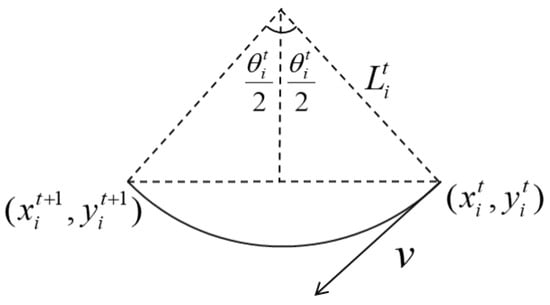
Figure 3.
Diagram of UAV motion constraints. The UAV moves from position to along a circular arc, where represents the path length, is the turning angle, and v denotes the velocity vector of the UAV.
(2) The minimum approach distance constraint: the distance between each UAV and the target must not be less than the minimum approach distance , and the distance should satisfy
where represents the distance between the ith UAV and the target at time t.
(3) The deflection angle constraint: To ensure that the UAVs head toward the target, the heading direction of the UAV i at time t must be within the left and right angle range along the line connecting it to the target. Therefore, the deflection angle of the UAV i at time t must satisfy
where the parameters are defined by
where represents the azimuth angle of the target related to the ith UAV, and is the adaptive adjustment range.
(4) No-fly-zone (NFZ) constraint: To ensure operational safety and comply with airspace restrictions, the UAVs should not fly in the NFZ
where represents the position coordinates of the ith UAV at time t, and represents the complete set of restricted points, which is the union of all these individual NFZ and can be represented as
where p is the number of the individual NFZ.
4.3. Path Optimization Model
Based on the problem formulation and the constraints derived above, the mathematical model for UAV path optimization can be described as
where represents the planed position of the UAVs that are assigned to the target at the next time step, and is the trace of the predicted CRLB matrix for the localization of the target at the next time step.
4.4. Path Optimization Algorithm Design
To quickly search the planned optimal positions for the UAVs to localize the target at the next time step, in this paper, the PSO algorithm is deployed.
Suppose there are S particles searching in each iteration, and each particle s () has information about its own best position , which it has never visited; its current position ; its velocity ; and the global best solution found by all particles. Specifically, in the th dimension, the movement of each particle is influenced by its own best position , the global best position , and its current velocity . The velocity and position are updated as follows, where k denotes the iteration step for the particle.
where is the inertia weight, which decreases with iteration time as . is the maximum number of iterations. and are individual learning and global learning factors, which vary with iteration time as and respectively. and are random independent variables in the range [0,1]. The velocity of particle in each dimension is limited by a fixed . The current position of each particle represents its current proposed solution. The performance of each solution is evaluated via a fitness function (denoted by ). In this algorithm, each particle is a -dimensional vector that contains all positions of the UAVs in two-dimension space. For instance, the expression of the sth particle is
where denotes the deflection angle of the ith UAV in the sth particle, and is the number of UAVs. For initialization, we randomly place all UAVs in a certain region. The velocity and position of every particle will be updated in each iteration. The fitness function of the sth particle is as follows:
where denotes the current position of the sth particle, and can be updated as
When , the iteration will stop and output the optimization result; thus, the optimal UAV positions will be obtained. Here, a summary process of the path optimization is given in Algorithm 2.
| Algorithm 2: CRLB-based path optimization via PSO |
 |
5. Numerical Results
In this section, we present numerical simulations to verify the validity and effectiveness of the proposals in this paper. First, we set the parameters and the initial topology structure of the UAVs and the targets. Then, the simulation results of the node selection method and the path optimization method are given. Finally, the time costs of the PSO algorithm and the exhaustive algorithm are compared to verify the effectiveness of the PSO algorithm.
5.1. Simulation Parameters and the Topology Structure Set
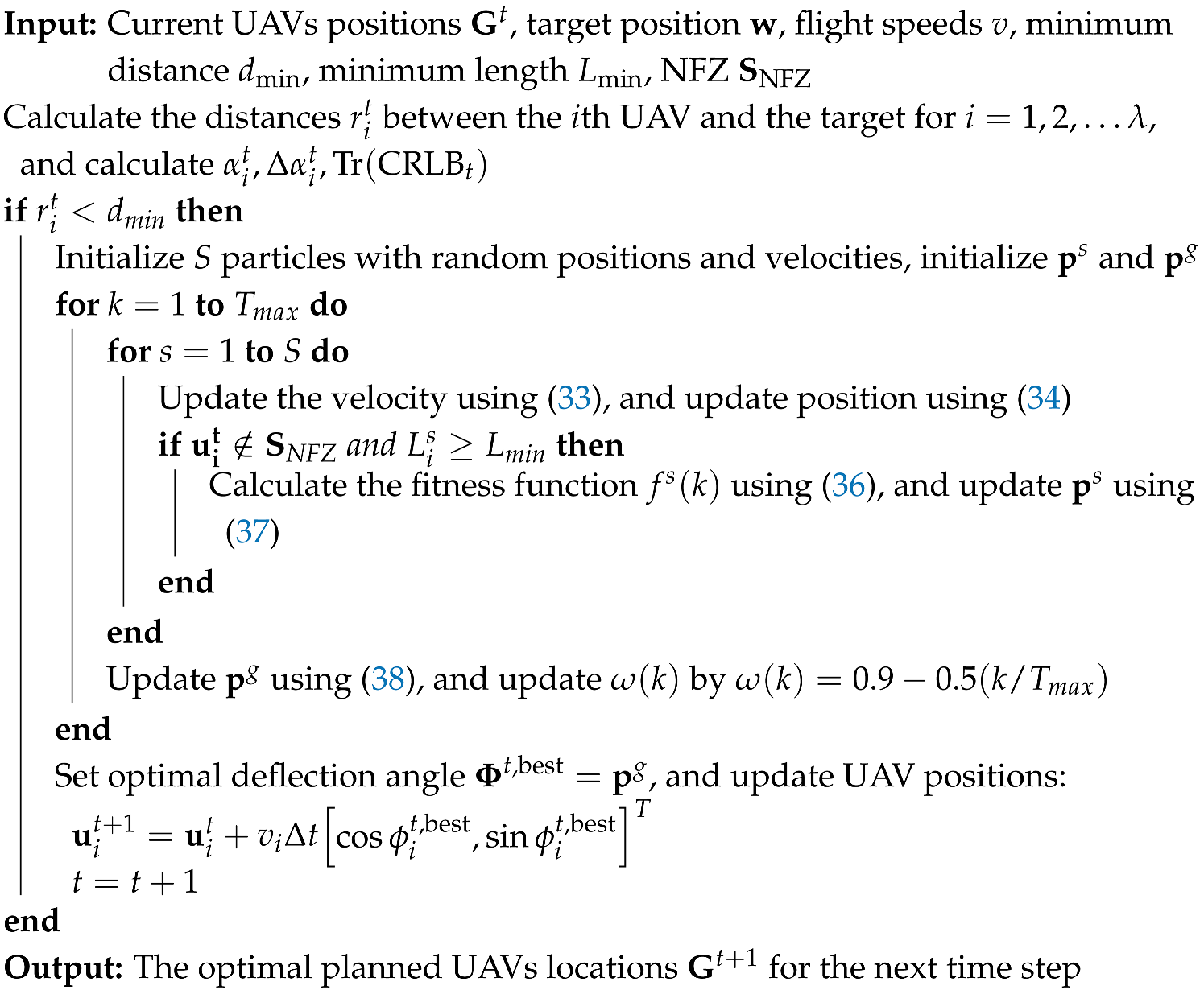
Consider that there are nine UAVs () and three targets () in a two-dimensional plane. The positions of the UAVs are [0, 10,000] m, [2500, 9000] m, [4000, 8500] m, [5000, 7500] m, [7000, 6200] m, [7800, 5000] m, [9000, 4200] m, [9500, 2500] m, and [9000, 1000] m. The positions of the targets are [10,000, 32,000] m, [23,000, 23,000] m, and [30,000, 10,000] m. The UAVs’ minimum turning radius is set to be m, and the minimum approach distance is set to be m. The initial topology of the UAVs and the targets is shown in Figure 4.
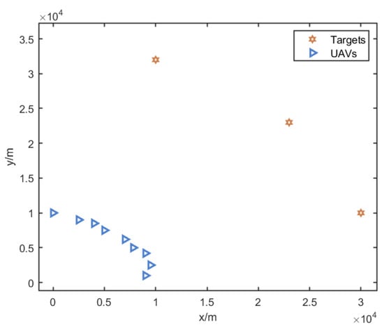
Figure 4.
Initial positions of the UAVs and the targets. The blue triangles represent the initial positions of the 9 UAVs (UAV0–UAV8), and the orange stars represent the initial positions of the 3 targets.
5.2. Simulation Results of the Node Selection Algorithm
In this paper, it is assumed that at each time step, three UAVs are assigned to a target; thus, the UAVs will be divided into three groups to localize for three targets. The result of the CRLB-based node selection is shown in Figure 5.
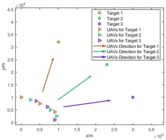
Figure 5.
UAV grouping results and their movement directions after node selection. Different colors represent different UAV groups assigned to their respective targets, and arrows indicate the planned movement directions.
To evaluate the performance of the node selection, the root mean square error (RMSE) is used as a localization accuracy metric, and the performance comparisons between the proposed CRLB-based node selection algorithm with the random selection method are made. The RMSE can be obtained by
A total of 1000 independent Monte Carlo experiments () were conducted to complete the comparisons. For the convenience of providing descriptions, in the following part, the proposed CRLB-based node selection algorithm is called the proposed algorithm for short, and the random node selection method is called the traditional algorithm for short.
From Table 1, it can be seen that the RMSEs of the proposed algorithm are much lower than that of the traditional algorithm. The RMSEs of the three different target based on the proposed algorithm decrease about 20–30% compared to the traditional algorithm. The average execution time of the proposed algorithm is 50.62 ms per iteration. The results illustrate that by efficient node selection, the target localization accuracy can be improved at a large scale.

Table 1.
RMSE comparisons between the proposed node selection method and the traditional method.
5.3. Simulation Results of the CRLB-Based Path Optimization Method
Through the node selection method, the UAVs have been divided into several groups for different target localizations. In this part, for each UAV group, we analyze the performance of the CRLB-based path optimization algorithm. The PSO algorithm is implemented with 50 particles and 500 maximum iterations in a three-dimensional continuous solution space, where each dimension represents the deflection angle of each UAV. The cognitive factor decreases linearly from 2.5 to 0.5, and the social factor increases from 0.5 to 2.5, with an inertia weight w decreasing from 0.9 to 0.4. A total of 800 independent Monte Carlo experiments are conducted for the comparison between the proposed CRLB-based path optimization method and the fixed formation method. For the convenience of description, we call the proposed CRLB-based path optimization algorithm as the proposed algorithm for short and call the fixed formation algorithm the traditional algorithm for short.
Figure 6 shows the average convergence behavior of the PSO algorithm over 50 independent runs during path optimization for the first UAV group targeting target 1 at the initial time step. The solid line represents the mean convergence curve, while the shaded area indicates one standard deviation above and below the mean value. The algorithm reliably achieves stable convergence after approximately 300 iterations, with the final average CRLB value reaching 127.8 with a standard deviation of approximately ±1.2 . This stable convergence pattern across multiple runs validates the robustness of the proposed PSO parameter settings in consistently finding high-quality solutions.
Figure 6.
Evolution of best fitness value (CRLB) during PSO iterations for the first UAV group at the initial time step.
Figure 7a, Figure 8a and Figure 9a give the topology of the UAVs and the target for each UAV group. Figure 7b, Figure 8b and Figure 9b show the UAVs’ motion paths based on the proposed path optimization method, and the RMSE and CRLB of the localization for each target are shown in Figure 10, Figure 11 and Figure 12.
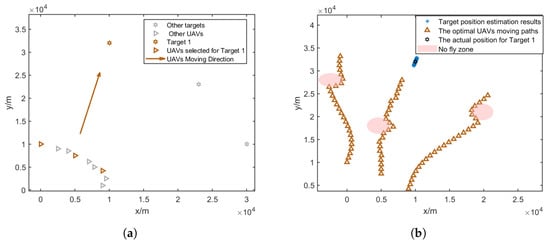
Figure 7.
Three selected UAVs localizing target 1 and their moving direction. (a) Movement direction of the three selected UAV groups for target 1. (b) Trajectories of the three selected UAV groups for target 1.
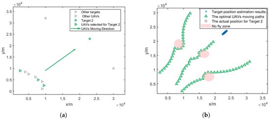
Figure 8.
Three selected UAVs localizing target 2 and their moving directions. (a) Movement direction of the three selected UAV groups for target 2. (b) Trajectories of the three selected UAV groups for target 2.
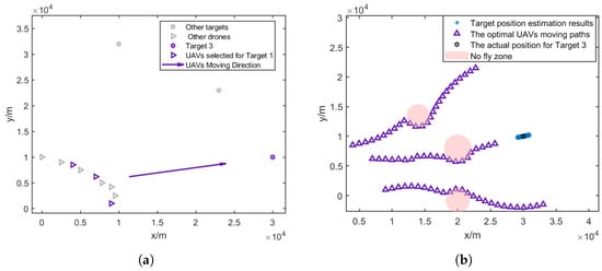
Figure 9.
Three selected UAVs localizing target 3 and their moving direction. (a) Movement direction of the three selected UAV groups for target 3. (b) Trajectories of the three selected UAV groups for target 3.
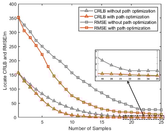
Figure 10.
Comparison of CRLB and RMSE under path optimization versus fixed configuration for target 1.
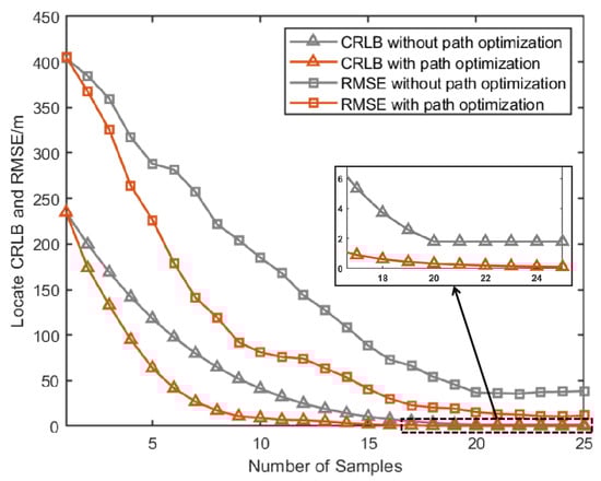
Figure 11.
Comparison of RMSE and CRLB between the proposed path optimization method and the traditional method.
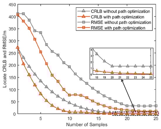
Figure 12.
Comparison of RMSE and CRLB between the proposed path optimization method and the traditional method.
From Figure 10, Figure 11 and Figure 12, it can be seen that for all three groups of UAVs, the RMSE and CRLB of the proposed path optimization method is lower than that of the traditional method. In Figure 10, the average RMSE for the proposed method is lower by about 43.37% than the traditional method, and the average CRLB for the proposed method is lower by about 62.99% than the traditional method. In Figure 11, the average RMSE for the proposed method is lower by about 47.59% than the traditional method, and the average CRLB for the proposed method is lower by about 68.65% than the traditional method. And in Figure 12, the average RMSE for the proposed method is lower by about 45.01% than the traditional method, and the average CRLB for the proposed method is lower by about 66.68% than the traditional method. Moreover, the proposed method cab avoid the NFZ adaptively, while the fixed formation method in this paper is assumed to be unable to avoid the NFZ.
To verify the effectiveness of the PSO algorithm used in this paper, we compared PSO with three other optimization algorithms: GA, ACO, and the traditional exhaustive method. These algorithms are used to search for (the optimal UAV positions) at each time step to obtain the minimum trace of CRLB for the next time step. The parameter settings for the algorithms are shown in Table 2. GA operates in continuous space with 20 individuals, employing a crossover rate of 0.8 and a mutation rate of 0.1. The PSO parameter settings are the same as in the previous experiment, while ACO discretizes the search space into 20 points per dimension, using 50 ants with pheromone-based search strategies. All algorithms are set to a maximum of 500 iterations with different early stopping criteria and optimization strategies to enhance search efficiency. For the exhaustive method, the angle range is discretized into 50 equally spaced points, resulting in combinations that need to be evaluated at each time step to find the optimal waypoints resulting the minimum trace of CRLB.
Table 2.
Parameter settings of the three optimization algorithms.
As shown in Figure 13a–c, we present the CRLB and RMSE performance comparisons for five different methods: the fixed formation method (without path optimization) and four optimization methods (Exhaustive, PSO, ACO, and GA) localizing three different targets. The simulation results demonstrate that for localizing different targets, the four optimization approaches present similar convergence patterns in both CRLB and RMSE metrics, with their curves nearly overlapping throughout the localization process, and they all achieve lower CRLB and RMSE values compared to the fixed formation method. Figure 13d shows the computational time comparisons for a single iteration between different optimization methods. The results reveal that to realize the approximate localizing performance, the PSO algorithm maintains the lowest computation time consistently across all sampling times, while GA shows the highest computational burden and ACO demonstrates moderate computational requirements, positioned between PSO and the exhaustive method.
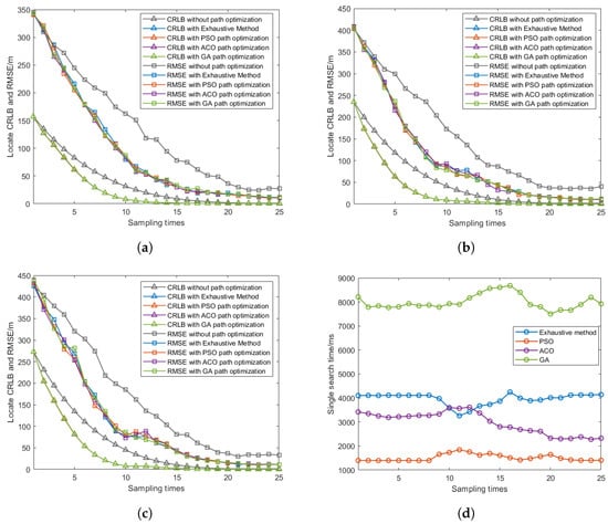
Figure 13.
CRLB comparison and single-iteration computation time comparisons with different optimization algorithms localizing different targets. (a) CRLB comparison with different optimization algorithms localizing target 1. (b) CRLB comparison with different optimization algorithms localizing target 2. (c) CRLB comparison with different optimization algorithms localizing target 3. (d) Single-iteration computation time comparisons between different optimization methods.
Table 3 shows the average percentage reduction in the CRLB and RMSE of path optimization algorithms (Exhaustive, PSO, ACO, and GA) compared to the fixed formation method. Specifically, the CRLB reduction for Exhaustive, PSO, ACO, and GA is 66.70%, 66.66%, 66.77%, and 66.57%, respectively, compared to the fixed formation method, while the RMSE reduction is 44.24%, 44.99%, 45.02%, and 44.64%, respectively, compared to the fixed formation method, indicating that with path optimization methods, the localization performance of the UAVs can be improved at a large scale. Table 3 gives the comparisons of the average single-iteration computation time between the four path optimization methods, with PSO taking 1.34 s, ACO taking 3.05 s, the Exhaustive method taking 4.28 s, and GA taking 7.76 s. It is evident that the PSO method applied in this paper takes the shortest computation time, followed by ACO and then the exhaustive method, while GA requires significantly more time. These results indicate that while all methods can achieve similar localization performance, and PSO offers the best computational efficiency, making it particularly suitable for real-time UAV path planning applications.
Table 3.
Performance comparison between different optimization methods.
As shown in Table 3, while all algorithms achieve similar CRLB and RMSE reductions compared to the fixed formation method, PSO demonstrates superior computational efficiency. These results suggest that PSO provides the best balance between computational efficiency and optimization performance, making it particularly suitable for real-time UAV formation, quickly responding to environmental changes.
The performance of the proposed algorithm in terms of localization accuracy and computational efficiency can be explained from two aspects. Firstly, while the traditional fixed formation method adopts predetermined UAV configurations without considering the impact of flight paths on localization performance, the CRLB-based path optimization algorithm continuously adjusts UAV flight paths to minimize the trace of CRLB. This optimization mechanism enables UAVs to select better observation angles, thereby obtaining more accurate measurements, reducing measurement errors, and improving localization accuracy, as evidenced by the lower RMSE values shown in Figure 13a–c. Secondly, among the four optimization algorithms, PSO converges to optimal solutions in less time with higher computational efficiency. This is because GA, ACO, and Exhaustive methods require global information and involve complex computations, while PSO’s characteristic of making decisions based on local relative measurements better meet real-time control requirements, resulting in shorter computation times, as shown in Figure 13d.
5.4. Impact Analysis of Minimum Turning Radius
To thoroughly investigate the impact of the minimum turning radius on path optimization and localization accuracy, we conducted comparative experiments with different minimum turning radii while keeping other parameters constant. Three UAVs were initially deployed at coordinates [0, 10,000] m, [5000, 7500] m, and [9000, 4200] m, with the target located at [50,000, 32,000] m. Using the PSO optimization algorithm introduced in Section 4, we set the minimum turning radius to 5000 m, 7500 m, and 10,000 m to examine its influence on UAV path optimization and localization performance. In total, 800 Monte Carlo simulations were performed to ensure the statistical significance of the results.
As shown in Figure 14a–c, the optimized UAV paths exhibit distinct characteristics under different minimum turning radius constraints. With increasing , the UAVs require wider turning arcs to change their flight directions, resulting in longer path lengths and more gradual course adjustments.
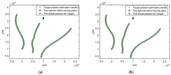
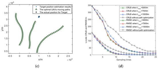
Figure 14.
Optimized UAV paths under different minimum turning radii and their RMSE comparisons. (a) = 5000 m. (b) = 7500 m. (c) = 10,000 m. (d) Comparison of RMSE and CRLB.
Figure 14d and Table 4 demonstrate the impact of turning radius constraints on localization accuracy. The simulation results show that a smaller turning radius allows for more flexible path planning and better localization performance. When increases from 5000 m to 10,000 m, the CRLB reduction deceases by 2.86 percentage points (from 64.57% CRLB reduction compared to the fixed formation method to 61.71%), while the RMSE reduction deceases by 3.59 percentage points (from 45.38% RMSE reduction compared to the fixed formation method to 41.79%). This trend indicates that larger minimum turning radius constraints moderately impact the algorithm’s ability to optimize UAV paths for target localization, as they limit the UAVs’ maneuverability in adjusting their positions for optimal measurement geometry.
Table 4.
Average performance improvement compared to the traditional method.
5.5. Impact Analysis of No-Fly-Zone Size
To evaluate the impact of no-fly-zone size on localization performance, we conducted comparative experiments with different no-fly-zone radii while maintaining other parameters constant. Three UAVs were initially deployed at coordinates [0, 10,000] m, [5000, 7500] m, and [9000, 4200] m, with the target located at [50,000, 32,000] m. Three circular no-fly zones were centered at [−2400, 28,000] m, [4600, 18,000] m, and [19,800, 21,000] m. Using the PSO optimization algorithm introduced in Section 4, we set the radii of no-fly zone to 1000 m, 2000 m, and 3000 m to examine their influence on localization performance. Also, 800 Monte Carlo simulations were performed to ensure the statistical significance of the results.
As shown in Figure 15a–c, the optimized UAV paths demonstrate different characteristics as increases. Larger no-fly zones force the UAVs to take more substantial detours, resulting in longer path lengths and more constrained movement patterns.
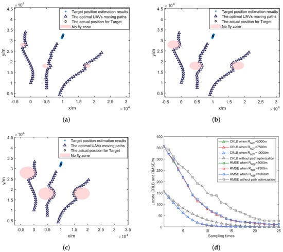
Figure 15.
Optimized UAV paths and comparison of RMSE and CRLB under different no-fly-zone radii. (a) = 1000 m. (b) = 2000 m. (c) = 3000 m. (d) Comparisons of RMSE and CRLB.
Figure 15d and Table 5 illustrate the impact of no-fly-zone size on localization accuracy. The simulation results indicate that increasing leads to degraded localization performance, as it restricts the available space for UAV path optimization solutions. When increases from 1000 m to 3000 m, the CRLB reduction decreases by 3.94 percentage points (from 63.88% CRLB reduction compared to the fixed formation method to 59.94%), while the RMSE reduction decreases by 2.56 percentage points (from 45.02% RMSE reduction compared to the fixed formation method to 42.46%). This degradation in performance can be attributed to the reduced flexibility in configuring UAVs relative to the optimal measurement geometry, as larger restricted areas limit the available space for tactical maneuvers.
Table 5.
Average performance under different no-fly-zone radii.
6. Conclusions
In this paper, we investigate the problem of node selection and path optimization for multi-target passive localization via UAVs. First, the Chan-TDOA target passive localization model is established.Then, the CRLB-based node selection algorithm is proposed to properly divide the UAVs into several groups localizing different targets, and the CRLB-based path optimization algorithm is proposed to search for the optimal UAV position configuration at each time step. The proposed path optimization method considers NFZ avoidance, ensuring both operational safety and localization accuracy. To improve the efficiency of path optimization, the PSO algorithm is applied to accelerate the searching process. Finally, numerical simulations were performed to verify the validity and effectiveness of the proposals in this paper.
Author Contributions
Conceptualization, X.X. and X.L.; methodology, X.X.; software, X.L.; validation, X.X., Y.Y. and Z.Z.; formal analysis, X.X.; investigation, X.X.; resources, X.X.; data curation, X.X. and X.L.; writing—original draft preparation, X.X.; writing—review and editing, X.X.; visualization, X.X.; supervision, X.L.; project administration, Y.Y.; funding acquisition, X.L. All authors have read and agreed to the published version of the manuscript.
Funding
This work is supported by the Qian Yuan Laboratory.
Institutional Review Board Statement
Not applicable.
Informed Consent Statement
Not applicable.
Data Availability Statement
Due to privacy constraints, we are unable to share the data utilized in this study for submission purposes. We assure you that the research methodology and results outlined in this paper comply with ethical guidelines and have been executed in line with recognized research protocols.
Conflicts of Interest
The authors declare no conflicts of interest.
Appendix A. Mathematical Derivations of Chan-TDOA Algorithm
Since the UAVs () are localizing the same target, we omit the superscript in this part for convenience. Therefore, the target’s location is denoted as . Then, the Chan-TDOA algorithm can be presented as follows:
For the convenience of comprehension, we first give the definitions for the important variables that would be used in subsequent derivations:
(1) represents the square of the location of the ith UAV (including ).
(2) and denote the relative locations of the ith UAV with respect to the master base station.
(3) indicates the difference in distance from the ith UAV to the target and from the master base station to the target.
(4) represents the difference in the times at which the signal was received by the ith UAV and received by the master base station.
(5) represents the variance in the TDOA measurement for the target.
It is apparent that
Squaring both sides of (A1), we obtain the following:
When the number of UAVs is , the system of (A3) can be solved using the elimination method to express x and y:
where and are the coefficients derived from (A3) using the elimination method. By setting and squaring both sides of (1), we obtain
Substituting (A3) into (A5) obtains
where and C are the coefficients of the quadratic equation in terms of obtained by substituting x and y from (A4) into (A5). This equation is a quadratic equation in terms of . Solving this equation and retaining the positive solution provide the viable value for . If two positive solutions are obtained, the unreasonable solution should be excluded based on practical conditions and prior information. The positive solution of is then substituted back into (A4) to determine the coordinates of the target location.
When the number of UAVs is , the number of TDOA measurements exceeds the number of unknown variables. In this scenario, a two-step WLS estimation can be employed to fully utilize redundant data and achieve a more accurate localization estimate. At this stage, in (A5) is a nonlinear term related to the target location. We treat it as an unknown variable that is included in
Let represent the true values of corresponding to the true target location. We then establish the linear equation with TDOA noise
where is the error vector caused by TDOA measurement noise, and
The covariance matrix of the error vector is
where
is the covariance matrix of the measurements.
Assuming that the elements of the error vector are mutually independent, the covariance matrix can be approximated by the matrix . Using the WLS method, the maximum likelihood estimate of can be expressed as
To achieve a more precise localization result, a second WLS estimation step is performed. At this point, we construct a noise vector similar to (A8)
where
The covariance matrix of the error vector is
where . The WLS localization estimate can be obtained as follows
The final estimated position of the target is
References
- Feldstein, S. How global demand for military drones is transforming international security and geopolitics. Georget. J. Int. Aff. 2023, 24, 146–155. [Google Scholar] [CrossRef]
- Gargalakos, M. The role of unmanned aerial vehicles in military communications: Application scenarios, current trends, and beyond. J. Def. Model. Simul. 2024, 21, 313–321. [Google Scholar] [CrossRef]
- Cao, X.; Wang, Z.; Zheng, B.; Tan, Y. Improved UAV-to-Ground Multi-Target Tracking Algorithm Based on StrongSORT. Sensors 2023, 23, 9239. [Google Scholar] [CrossRef] [PubMed]
- Zhou, R.; Almustafa, M.K.; Nehdi, M.L.; Su, H. Automated localization of dike leakage outlets using UAV-borne thermography and YOLO-based object detectors. ISPRS J. Photogramm. Remote Sens. 2024, 218, 551–573. [Google Scholar] [CrossRef]
- Mahmood, S.A.; Abdulmunem, F.A.; Lafta, S.H. Lightweight deep learning model-based UAVs visual detection. Multimed. Tools Appl. 2024. [Google Scholar] [CrossRef]
- Patole, S.M.; Torlak, M.; Wang, D.; Ali, M. Automotive radars: A review of signal processing techniques. IEEE Signal Process. Mag. 2017, 34, 22–35. [Google Scholar] [CrossRef]
- Rosić, M.; Sedak, M.; Simić, M.; Pejović, P. Chaos-Enhanced Adaptive Hybrid Butterfly Particle Swarm Optimization Algorithm for Passive Target Localization. Sensors 2022, 22, 5739. [Google Scholar] [CrossRef] [PubMed]
- Justin, K.; Simone, D. Autonomous angles-only multitarget tracking for spacecraft swarms. Acta Astronaut. 2021, 189, 514–529. [Google Scholar]
- Fokin, G. Passive Geolocation with Unmanned Aerial Vehicles using TDOA-AOA Measurement Processing. In Proceedings of the 2019 21st International Conference on Advanced Communication Technology (ICACT), PyeongChang, Republic of Korea, 17–20 February 2019; pp. 360–365. [Google Scholar] [CrossRef]
- Agrawal, S.; Kumar, P.; Sharma, A. Passive Emitter Localisation Using TDOA and FDOA Measurements from UAV. In Proceedings of the 2020 IEEE International Conference for Innovation in Technology (INOCON), Bangluru, India, 6–8 November 2020; pp. 1–5. [Google Scholar]
- Zhang, X.; Duan, L. Fast Deployment of UAV Networks for Optimal Wireless Coverage. IEEE Trans. Mob. Comput. 2019, 18, 588–601. [Google Scholar] [CrossRef]
- Suh, T.; Kim, W. Observability Study on Passive Target Localization by Conic–Angle Measurements. Sensors 2021, 21, 6439. [Google Scholar] [CrossRef]
- Jeon, M.H.; Lim, W.J.; Ryoo, C. Task Assignment for Multiple Multi-purpose Unmanned Aerial Vehicles Using Greedy Algorithm. Int. J. Aeronaut. Space Sci. 2024, 25, 1380–1394. [Google Scholar] [CrossRef]
- Xin, J.; Zhong, J.; Li, S. Greedy mechanism based particle swarm optimization for path planning problem of an unmanned surface vehicle. Sensors 2019, 19, 4620. [Google Scholar] [CrossRef]
- Wang, X.; Huang, C.; Chen, F. An improved particle swarm optimization algorithm for unmanned aerial vehicle route planning. J. Phys. Conf. Ser. 2022, 2245, 012013. [Google Scholar] [CrossRef]
- Meisquita, R.; Gasper, P. A novel path planning optimization algorithm based on particle swarm optimization for UAVs for bird monitoring and repelling. Processes 2021, 10, 62. [Google Scholar] [CrossRef]
- Huang, H.; Yang, Y.; Wang, H.; Ding, Z.; Sari, H.; Adachi, F. Deep Reinforcement Learning for UAV Navigation Through Massive MIMO Technique. IEEE Trans. Veh. Technol. 2020, 69, 1117–1121. [Google Scholar] [CrossRef]
- Cheng, C.; Zhang, H.; Sun, Y.; Tao, H.; Chen, Y. A cross-platform deep reinforcement learning model for autonomous navigation without global information in different scenes. Control Eng. Pract. 2024, 150, 105991. [Google Scholar] [CrossRef]
- Lee, M.-F.R.; Yusuf, S.H. Mobile Robot Navigation Using Deep Reinforcement Learning. Processes 2022, 10, 2748. [Google Scholar] [CrossRef]
- Maier, G.; Pfaff, F.; Wagner, M.; Pieper, C.; Gruna, R.; Noack, B.; Kruggel-Emden, H.; Längle, T.; Hanebeck, U.D.; Wirtz, S.; et al. Real-time multitarget tracking for sensor-based sorting—A new implementation of the auction algorithm for graphics processing units. J. Real-Time Image Process. 2019, 16, 2261–2272. [Google Scholar] [CrossRef]
- Rokbani, N.; Kromer, P.; Twir, I.; Alimi, A.M. A hybrid hierarchical heuristic-ACO with local search applied to travelling salesman problem, AS-FA-Ls. Int. J. Syst. Dyn. Appl. 2020, 9, 58–73. [Google Scholar] [CrossRef]
- Siemiatkowska, B.; Stecz, W. A Framework for Planning and Execution of Drone Swarm Missions in a Hostile Environment. Sensors 2021, 21, 4150. [Google Scholar] [CrossRef] [PubMed]
- Li, Z.H.; Zhang, K.Y.; Yang, L.; Wang, G.Y.; Hu, G. Improving heuristic functions in A* algorithm path planning. J. Res. Sci. Eng. 2022, 4, 10–20. [Google Scholar]
- Darrah, M.; Wilhelm, J.; Munasinghe, T.; Duling, K.; Yokum, S.; Sorton, E.; Rojas, J.; Wathen, M. A flexible genetic algorithm system for multi-UAV surveillance: Algorithm and flight testing. Unmanned Syst. 2015, 3, 49–62. [Google Scholar] [CrossRef]
- Huang, C.; Zhou, X.; Ran, X.; Wang, J.; Chen, H.; Deng, W. Adaptive cylinder vector particle swarm optimization with differential evolution for UAV path planning. Eng. Appl. Artif. Intell. 2023, 121, 105942. [Google Scholar] [CrossRef]
- Yang, X.S. A new metaheuristic bat-inspired algorithm. In Nature Inspired Cooperative Strategies for Optimization (NICSO 2010); Springer: Berlin/Heidelberg, Germany, 2010; p. 65. [Google Scholar]
- Dogancay, K.; Hmam, H. UAV path optimization for angle-only self-localization and target tracking based on the Bayesian Fisher information matrix. Sensors 2024, 24, 3120. [Google Scholar] [CrossRef]
Disclaimer/Publisher’s Note: The statements, opinions and data contained in all publications are solely those of the individual author(s) and contributor(s) and not of MDPI and/or the editor(s). MDPI and/or the editor(s) disclaim responsibility for any injury to people or property resulting from any ideas, methods, instructions or products referred to in the content. |
© 2025 by the authors. Licensee MDPI, Basel, Switzerland. This article is an open access article distributed under the terms and conditions of the Creative Commons Attribution (CC BY) license (https://creativecommons.org/licenses/by/4.0/).