
A Rolling-Bearing-Fault Diagnosis Method Based on a Dual Multi-Scale Mechanism Applicable to Noisy-Variable Operating Conditions


Abstract
1. Introduction
2. Methods and Theory
2.1. Anderson–Darling (AD)
2.2. Variational Mode Decomposition (VMD)
2.3. Convolutional Neural Network
3. The Proposed Diagnosis Method
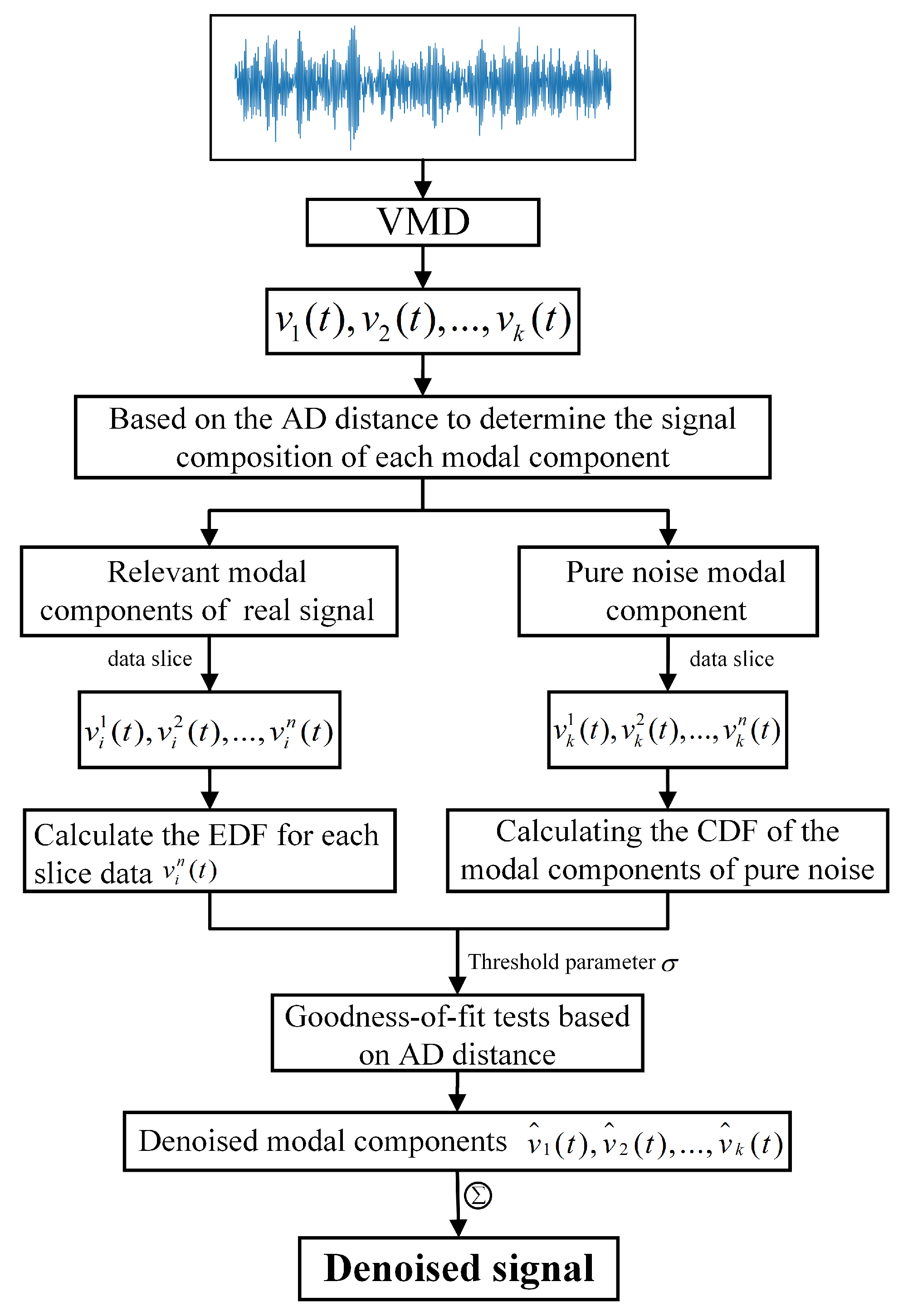
3.1. Multi-Scale Denoising Method
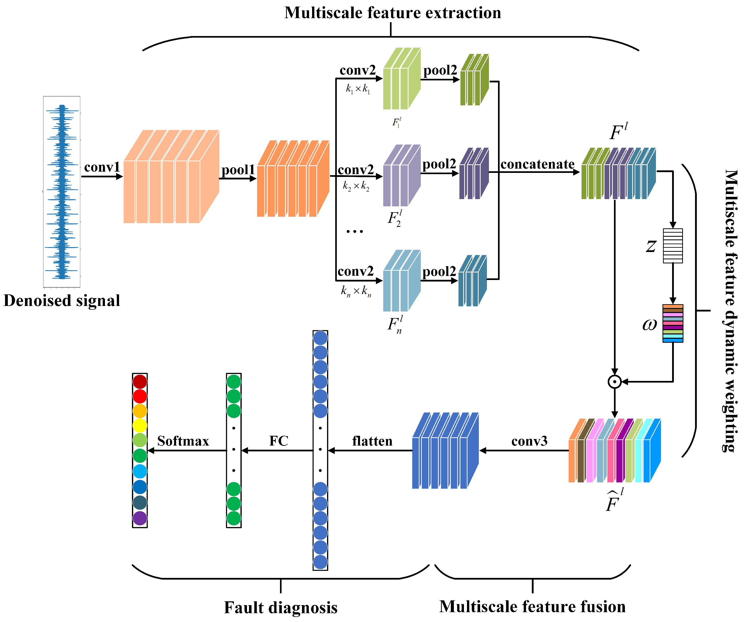
3.2. Multi-Scale Feature Extraction and Dynamic Weighting Method
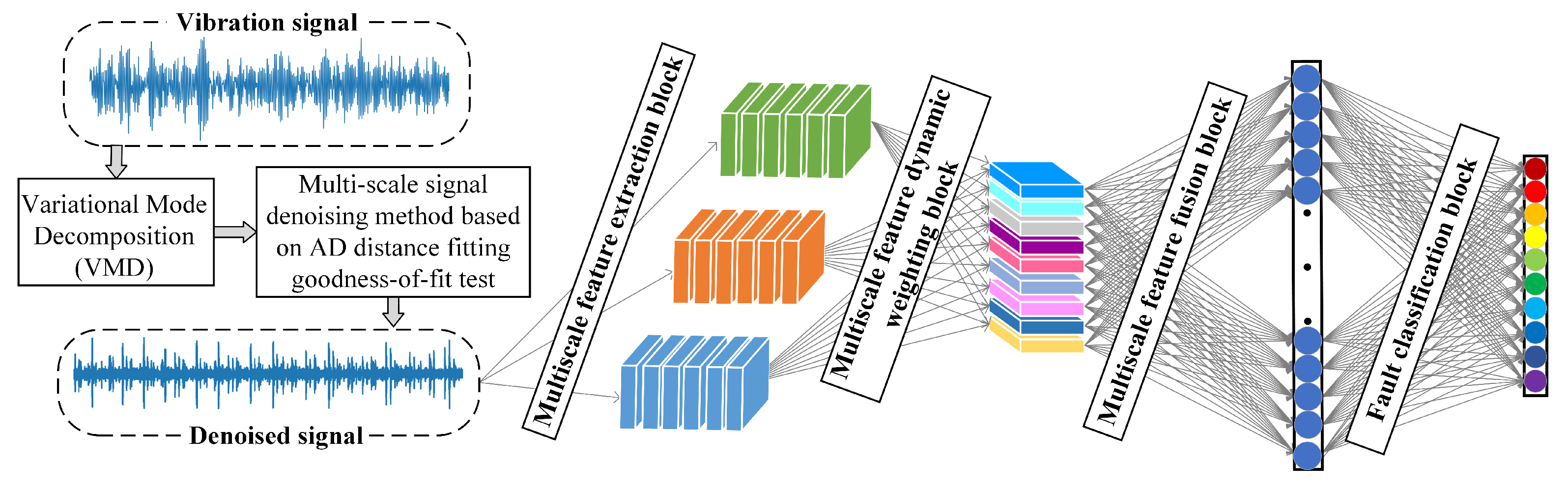
3.3. Rolling-Bearing-Fault Diagnosis Method Based on Dual Multi-Scale Mechanism Applicable to Noisy-Variable Operating Conditions
4. Experimental Validation and Analysis
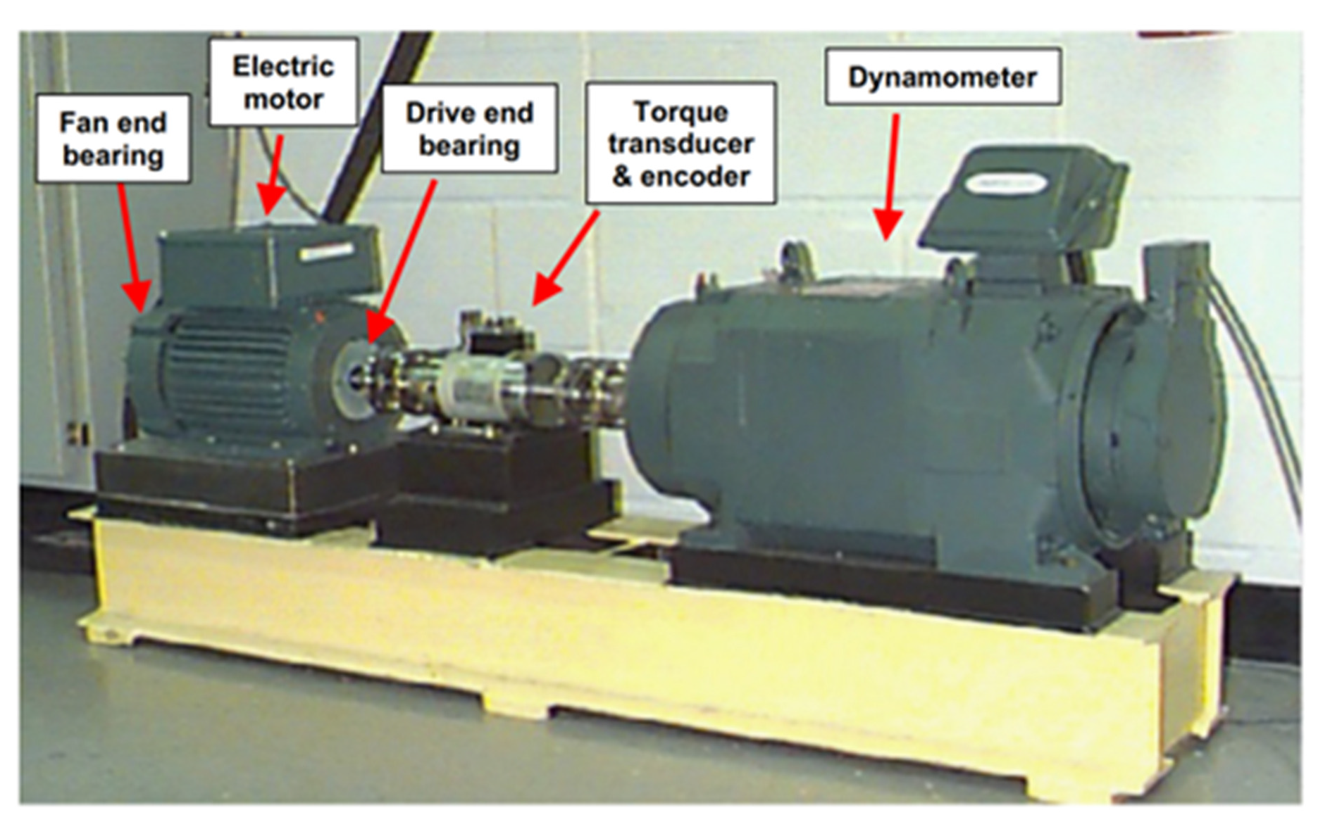
4.1. Description of Experimental Data
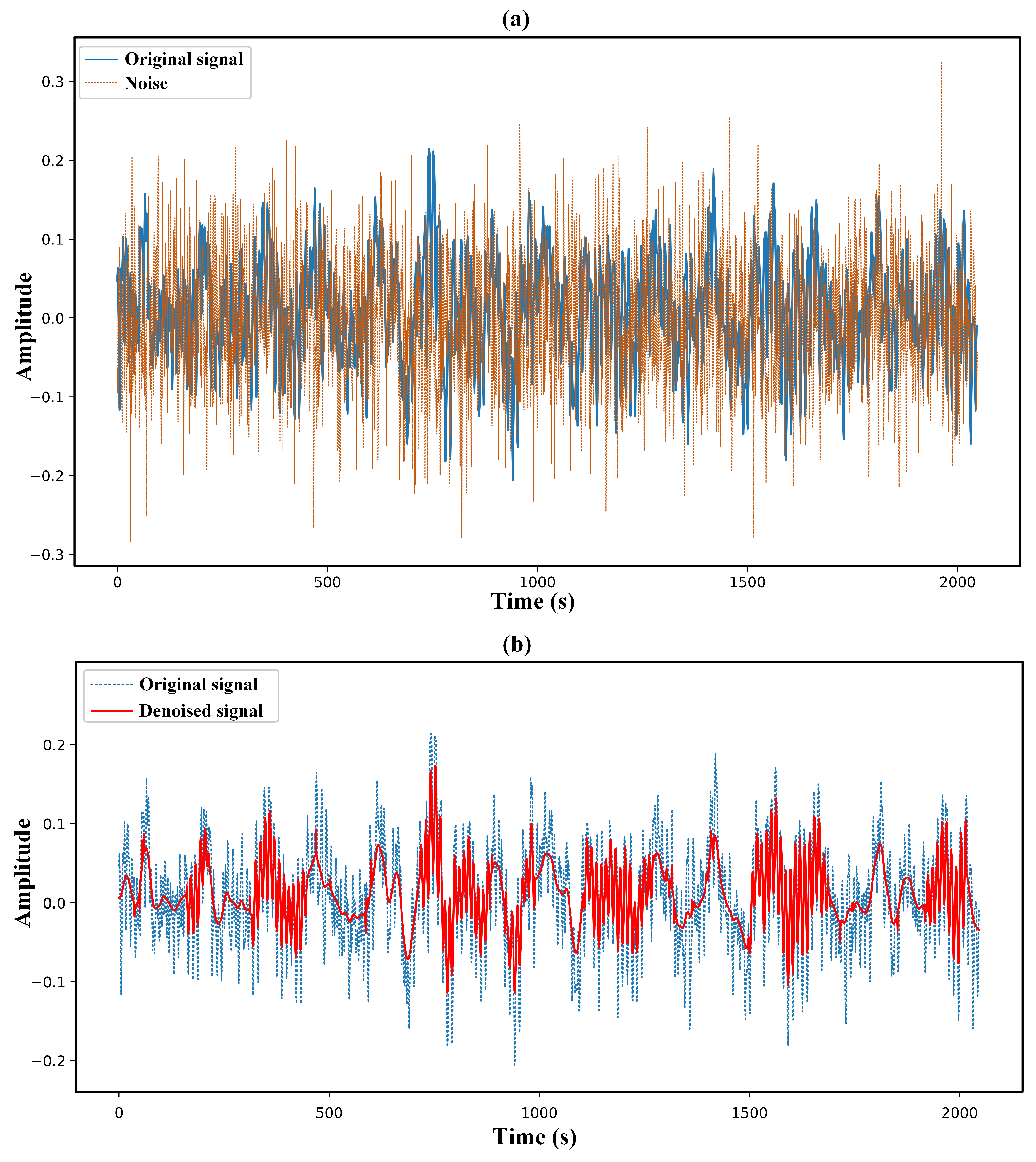
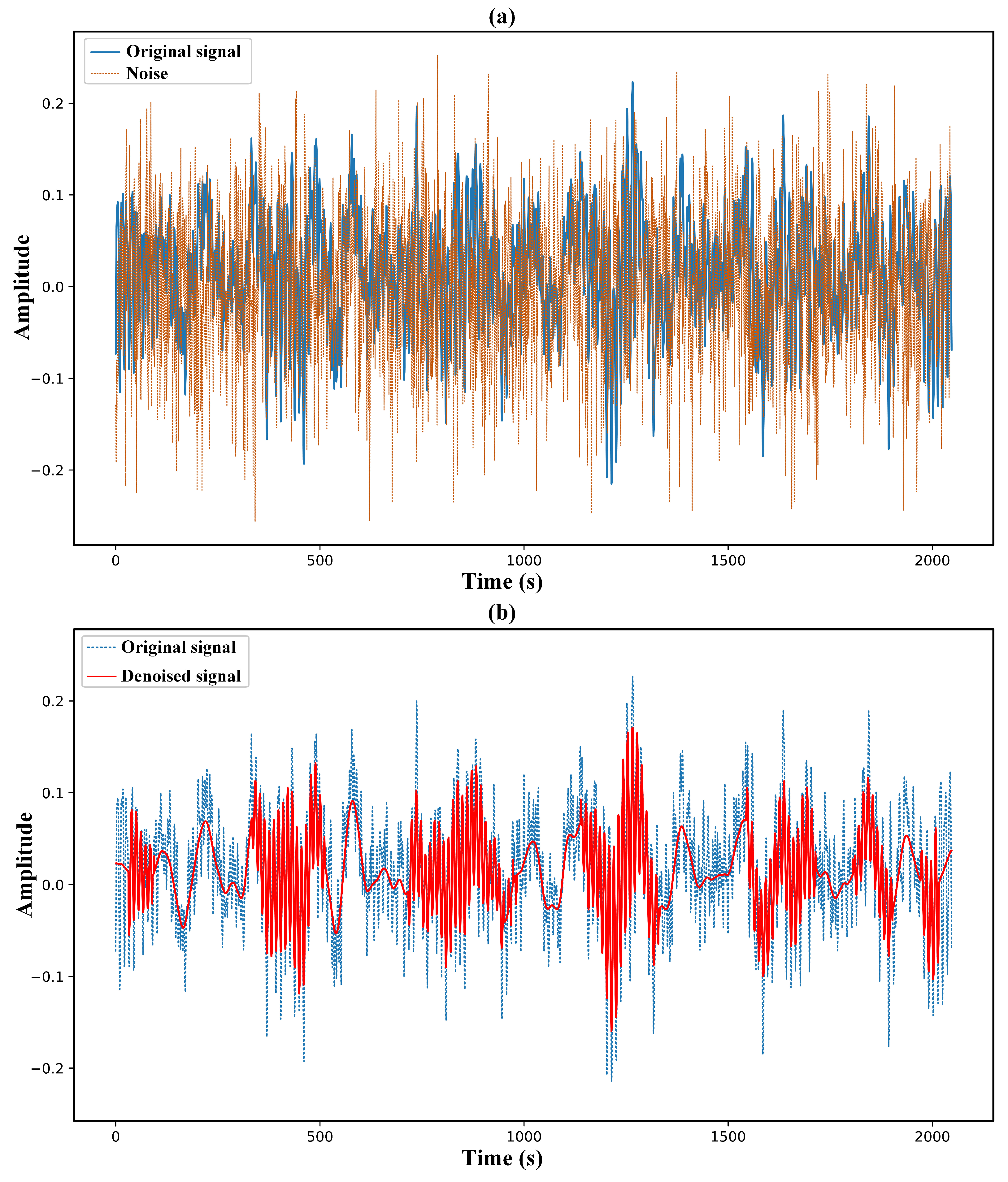
4.2. Denoising Effect of the Proposed Method in Noisy Environments
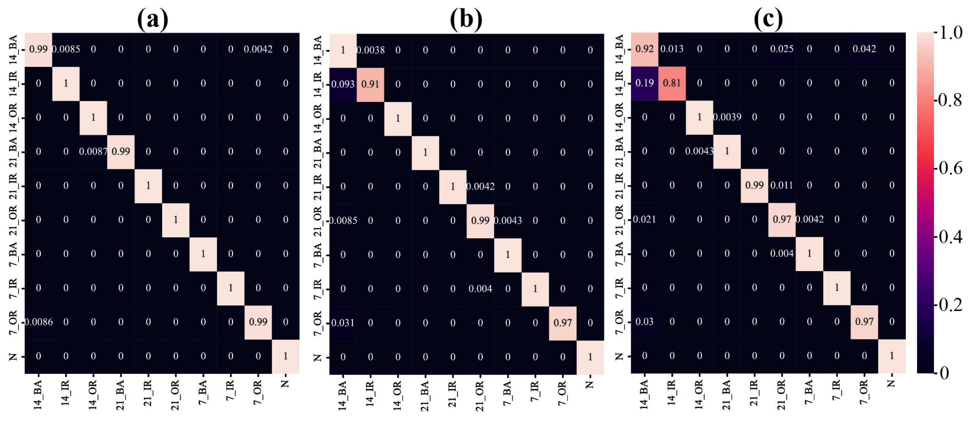
4.3. The Effectiveness of the Proposed Method in Fault Diagnosis Under Varying Operating Conditions
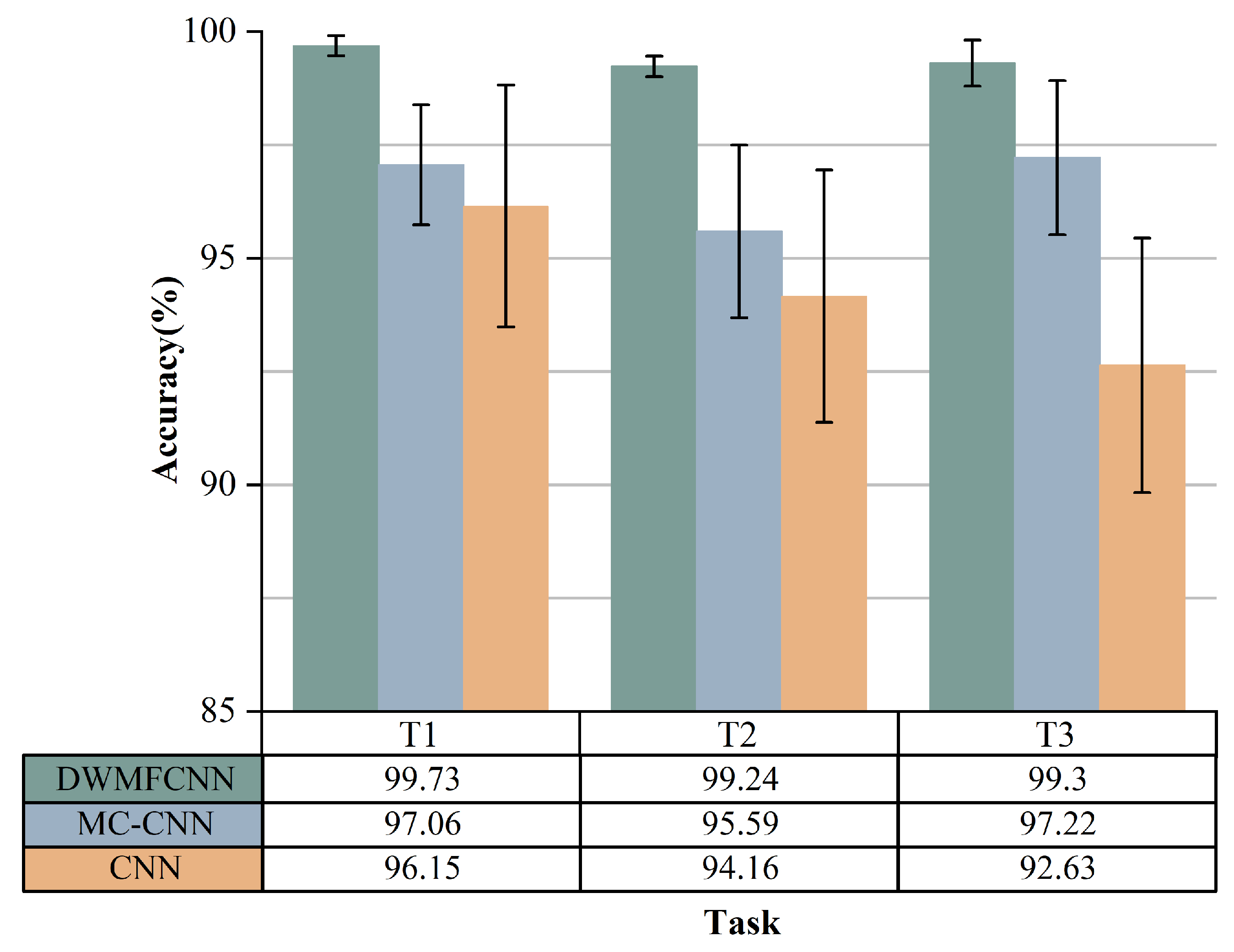
4.3.1. The Effectiveness of the Proposed Method for Fault Diagnosis Under Variable Load Conditions
4.3.2. The Effectiveness of the Proposed Method for Fault Diagnosis Under Variable Speed Conditions
5. Conclusions
Author Contributions
Funding
Data Availability Statement
Conflicts of Interest
References
- Guo, J.; Si, Z.; Xiang, J. A compound fault diagnosis method of rolling bearing based on wavelet scattering transform and improved soft threshold denoising algorithm. Measurement 2022, 196, 111276. [Google Scholar] [CrossRef]
- Wang, L.; Cao, H.; Liu, Z.; Fu, Y.; Ding, J. Joint discriminative and shared dictionary learning with dictionary extension strategy for bearing fault classification. Measurement 2021, 186, 110017. [Google Scholar] [CrossRef]
- Kumar, A.; Gandhi, C.; Zhou, Y.; Tang, H.; Xiang, J. Fault diagnosis of rolling element bearing based on symmetric cross entropy of neutrosophic sets. Measurement 2020, 152, 107318. [Google Scholar] [CrossRef]
- Kumar, A.; Tang, H.; Vashishtha, G.; Xiang, J. Noise subtraction and marginal enhanced square envelope spectrum (MESES) for the identification of bearing defects in centrifugal and axial pump. Mech. Syst. Signal Process. 2022, 165, 108366. [Google Scholar] [CrossRef]
- Kumar, A.; Vashishtha, G.; Gandhi, C.; Tang, H.; Xiang, J. Tacho-less sparse CNN to detect defects in rotor-bearing systems at varying speed. Eng. Appl. Artif. Intell. 2021, 104, 104401. [Google Scholar] [CrossRef]
- Jiang, X.; Wang, J.; Shi, J.; Shen, C.; Huang, W.; Zhu, Z. A coarse-to-fine decomposing strategy of VMD for extraction of weak repetitive transients in fault diagnosis of rotating machines. Mech. Syst. Signal Process. 2019, 116, 668–692. [Google Scholar] [CrossRef]
- Wang, J.; Du, G.; Zhu, Z.; Shen, C.; He, Q. Fault diagnosis of rotating machines based on the EMD manifold. Mech. Syst. Signal Process. 2020, 135, 106443. [Google Scholar] [CrossRef]
- Lei, Y.; Lin, J.; He, Z.; Zuo, M.J. A review on empirical mode decomposition in fault diagnosis of rotating machinery. Mech. Syst. Signal Process. 2013, 35, 108–126. [Google Scholar] [CrossRef]
- Yang, Y.; Pan, H.; Ma, L.; Cheng, J. A roller bearing fault diagnosis method based on the improved ITD and RRVPMCD. Measurement 2014, 55, 255–264. [Google Scholar] [CrossRef]
- Dragomiretskiy, K.; Zosso, D. Variational mode decomposition. IEEE Trans. Signal Process. 2013, 62, 531–544. [Google Scholar] [CrossRef]
- Lv, Z.; Han, S.; Peng, L.; Yang, L.; Cao, Y. Weak fault feature extraction of rolling bearings based on adaptive variational modal decomposition and multiscale fuzzy entropy. Sensors 2022, 22, 4504. [Google Scholar] [CrossRef]
- Li, Z.; Xiao, J.; Ding, X.; Wang, L.; Yang, Y.; Zhang, W.; Du, M.; Shao, Y. A new raw signal fusion method using reweighted VMD for early crack fault diagnosis at spline tooth of clutch friction disc. Measurement 2023, 220, 113414. [Google Scholar] [CrossRef]
- Jin, Z.; Chen, G.; Yang, Z. Rolling bearing fault diagnosis based on WOA-VMD-MPE and MPSO-LSSVM. Entropy 2022, 24, 927. [Google Scholar] [CrossRef]
- Shi, R.; Wang, B.; Wang, Z.; Liu, J.; Feng, X.; Dong, L. Research on fault diagnosis of rolling bearings based on variational mode decomposition improved by the niche genetic algorithm. Entropy 2022, 24, 825. [Google Scholar] [CrossRef]
- Zhou, J.; Xiao, M.; Niu, Y.; Ji, G. Rolling bearing fault diagnosis based on WGWOA-VMD-SVM. Sensors 2022, 22, 6281. [Google Scholar] [CrossRef]
- Yang, Y.; Yin, J.; Zheng, H.; Li, Y.; Xu, M.; Chen, Y. Learn generalization feature via convolutional neural network: A fault diagnosis scheme toward unseen operating conditions. IEEE Access 2020, 8, 91103–91115. [Google Scholar] [CrossRef]
- Gu, J.; Peng, Y.; Lu, H.; Chang, X.; Chen, G. A novel fault diagnosis method of rotating machinery via VMD, CWT and improved CNN. Measurement 2022, 200, 111635. [Google Scholar] [CrossRef]
- Gao, Y.; Kim, C.H.; Kim, J.M. A novel hybrid deep learning method for fault diagnosis of rotating machinery based on extended WDCNN and long short-term memory. Sensors 2021, 21, 6614. [Google Scholar] [CrossRef]
- Zhang, W.; Li, C.; Peng, G.; Chen, Y.; Zhang, Z. A deep convolutional neural network with new training methods for bearing fault diagnosis under noisy environment and different working load. Mech. Syst. Signal Process. 2018, 100, 439–453. [Google Scholar] [CrossRef]
- Zhang, W.; Peng, G.; Li, C.; Chen, Y.; Zhang, Z. A new deep learning model for fault diagnosis with good anti-noise and domain adaptation ability on raw vibration signals. Sensors 2017, 17, 425. [Google Scholar] [CrossRef]
- Sun, H.; Cao, X.; Wang, C.; Gao, S. An interpretable anti-noise network for rolling bearing fault diagnosis based on FSWT. Measurement 2022, 190, 110698. [Google Scholar] [CrossRef]
- Jin, T.; Yan, C.; Chen, C.; Yang, Z.; Tian, H.; Guo, J. New domain adaptation method in shallow and deep layers of the CNN for bearing fault diagnosis under different working conditions. Int. J. Adv. Manuf. Technol. 2023, 124, 3701–3712. [Google Scholar] [CrossRef]
- Li, Y.; Du, X.; Wang, X.; Si, S. Industrial gearbox fault diagnosis based on multi-scale convolutional neural networks and thermal imaging. ISA Trans. 2022, 129, 309–320. [Google Scholar] [CrossRef]
- Qiao, H.; Wang, T.; Wang, P.; Zhang, L.; Xu, M. An adaptive weighted multiscale convolutional neural network for rotating machinery fault diagnosis under variable operating conditions. IEEE Access 2019, 7, 118954–118964. [Google Scholar] [CrossRef]
- Huang, W.; Cheng, J.; Yang, Y.; Guo, G. An improved deep convolutional neural network with multi-scale information for bearing fault diagnosis. Neurocomputing 2019, 359, 77–92. [Google Scholar] [CrossRef]
- Chen, X.; Zhang, B.; Gao, D. Bearing fault diagnosis base on multi-scale CNN and LSTM model. J. Intell. Manuf. 2021, 32, 971–987. [Google Scholar] [CrossRef]
- Shen, Q.; Zhang, Z. Fault diagnosis method for bearing based on attention mechanism and multi-scale convolutional neural network. IEEE Access 2024, 12, 12940–12952. [Google Scholar] [CrossRef]
- Shi, P.; Xue, P.; Liu, A.; Han, D. A novel rotating machinery fault diagnosis method based on adaptive deep belief network structure and dynamic learning rate under variable working conditions. IEEE Access 2021, 9, 44569–44579. [Google Scholar] [CrossRef]
- Liang, H.; Cao, J.; Zhao, X. Multi-scale dynamic adaptive residual network for fault diagnosis. Measurement 2022, 188, 110397. [Google Scholar] [CrossRef]
- Sun, T.; Gao, J.; Meng, L.; Huang, Z.; Yang, S.; Li, M. A bearing fault diagnosis method based on adaptive residual shrinkage network. Measurement 2024, 238, 115416. [Google Scholar] [CrossRef]
- Liu, L.; Cheng, Y.; Song, D.; Zhang, W.; Tang, G.; Luo, Y. A Lightweight Network with Adaptive Input and Adaptive Channel Pruning Strategy for Bearing Fault Diagnosis. IEEE Trans. Instrum. Meas. 2023, 73, 3510911. [Google Scholar] [CrossRef]
- Liu, X.; Wang, J.; Meng, S.; Qiu, X.; Zhao, G. Multi-view rotating machinery fault diagnosis with adaptive co-attention fusion network. Eng. Appl. Artif. Intell. 2023, 122, 106138. [Google Scholar] [CrossRef]
- Jäntschi, L.; Bolboacă, S.D. Computation of probability associated with Anderson–Darling statistic. Mathematics 2018, 6, 88. [Google Scholar] [CrossRef]
- Stephens, M.A. EDF statistics for goodness of fit and some comparisons. J. Am. Stat. Assoc. 1974, 69, 730–737. [Google Scholar] [CrossRef]
- Anderson, T.W.; Darling, D.A. A test of goodness of fit. J. Am. Stat. Assoc. 1954, 49, 765–769. [Google Scholar] [CrossRef]
- Liu, S.; Zhao, R.; Yu, K.; Zheng, B.; Liao, B. Output-only modal identification based on the variational mode decomposition (VMD) framework. J. Sound Vib. 2022, 522, 116668. [Google Scholar] [CrossRef]
- Kang, J.; Luo, Y.; Wang, P.; Wei, Y.; Zhou, Y. Fault Diagnosis of Rotating Machinery under Complex Conditions Based on Multi-Scale Convolutional Neural Networks. J. Phys. Conf. Ser. 2023, 2658, 012038. [Google Scholar] [CrossRef]
- Naveed, K.; Akhtar, M.T.; Siddiqui, M.F.; ur Rehman, N. A statistical approach to signal denoising based on data-driven multiscale representation. Digit. Signal Process. 2021, 108, 102896. [Google Scholar] [CrossRef]
- Ma, W.; Yin, S.; Jiang, C.; Zhang, Y. Variational mode decomposition denoising combined with the Hausdorff distance. Rev. Sci. Instrum. 2017, 88, 035109. [Google Scholar] [CrossRef]
- Liu, Y.; Yang, G.; Li, M.; Yin, H. Variational mode decomposition denoising combined the detrended fluctuation analysis. Signal Process. 2016, 125, 349–364. [Google Scholar] [CrossRef]
- Smith, W.A.; Randall, R.B. Rolling element bearing diagnostics using the Case Western Reserve University data: A benchmark study. Mech. Syst. Signal Process. 2015, 64, 100–131. [Google Scholar] [CrossRef]
- Case Western Reserve University Bearing Data Center. Case Western Reserve University Bearing Data Center Website. 2009. Available online: https://engineering.case.edu/bearingdatacenter (accessed on 1 June 2024).
- Li, X.; Zhang, W.; Ding, Q. A robust intelligent fault diagnosis method for rolling element bearings based on deep distance metric learning. Neurocomputing 2018, 310, 77–95. [Google Scholar] [CrossRef]
- Liu, C.; Cheng, G.; Chen, X.; Pang, Y. Planetary gears feature extraction and fault diagnosis method based on VMD and CNN. Sensors 2018, 18, 1523. [Google Scholar] [CrossRef]


| Fault Types Description | Samples | Category | |||
|---|---|---|---|---|---|
| 0 hp | 1 hp | 2 hp | 3 hp | ||
| N (normal) | 300 | 300 | 300 | 300 | Class 1 |
| 7-OR (outer race fault diameter: 0.007 inch) | 300 | 300 | 300 | 300 | Class 2 |
| 14-OR (outer race fault diameter: 0.014 inch) | 300 | 300 | 300 | 300 | Class 3 |
| 21-OR (outer race fault diameter: 0.021 inch) | 300 | 300 | 300 | 300 | Class 4 |
| 7-BA (ball fault diameter: 0.007 inch) | 300 | 300 | 300 | 300 | Class 5 |
| 14-BA (ball fault diameter: 0.014 inch) | 300 | 300 | 300 | 300 | Class 6 |
| 21-BA (ball fault diameter: 0.021 inch) | 300 | 300 | 300 | 300 | Class 7 |
| 7-IR (inner race fault diameter: 0.007 inch) | 300 | 300 | 300 | 300 | Class 8 |
| 14-IR (inner race fault diameter: 0.014 inch) | 300 | 300 | 300 | 300 | Class 9 |
| 21-IR (inner race fault diameter: 0.021 inch) | 300 | 300 | 300 | 300 | Class 10 |
| Denoising Methods | SNR Gain (dB) | RMSE |
|---|---|---|
| VMD | 1.886 | 0.503 |
| VMD-AD | 5.147 | 0.162 |
| Task | T1 | T2 | T3 |
|---|---|---|---|
| Train | 0 hp + 2 hp + 3 hp | 0 hp + 1 hp + 3 hp | 0 hp + 1 hp + 2 hp |
| Test | 1 hp | 2 hp | 3 hp |
| Module Name | Layer Name | Convolution Kernel /Pooling Size | Number of Convolution Kernels | Activation Function |
|---|---|---|---|---|
| Multiscale Feature Extraction Module | Conv2d | (16,16) | 4 | ReLU |
| Pooling | (4,4) | / | ||
| Conv2d | (6,6) | 4 | ||
| Conv2d | (4,4) | 4 | ||
| Conv2d | (2,2) | 4 | ||
| Concatenate | / | / | ||
| Multiscale Feature Dynamic Weighting Module | Conv2d | (4,4) | 4 | |
| Global average pooling | (2,2) | / | ||
| FC layer | 5 | / | ||
| FC layer | 10 | / | ||
| Weighting layer | / | / | ||
| Multiscale Feature Fusion Module | Conv2d | (4,4) | 4 | |
| Batch Normalization | / | / | ||
| Pooling | (2,2) | / | ||
| Flatten | / | / | ||
| Fault Classification Module | FC layer | 100 | / | |
| Batch Normalization | / | / | ||
| FC layer | 10 | / | Softmax |
| Category | Parameter | Value/Description | Remarks |
|---|---|---|---|
| Data Acquisition | Sampling frequency | 25.6 kHz | Anti-aliasing filtered |
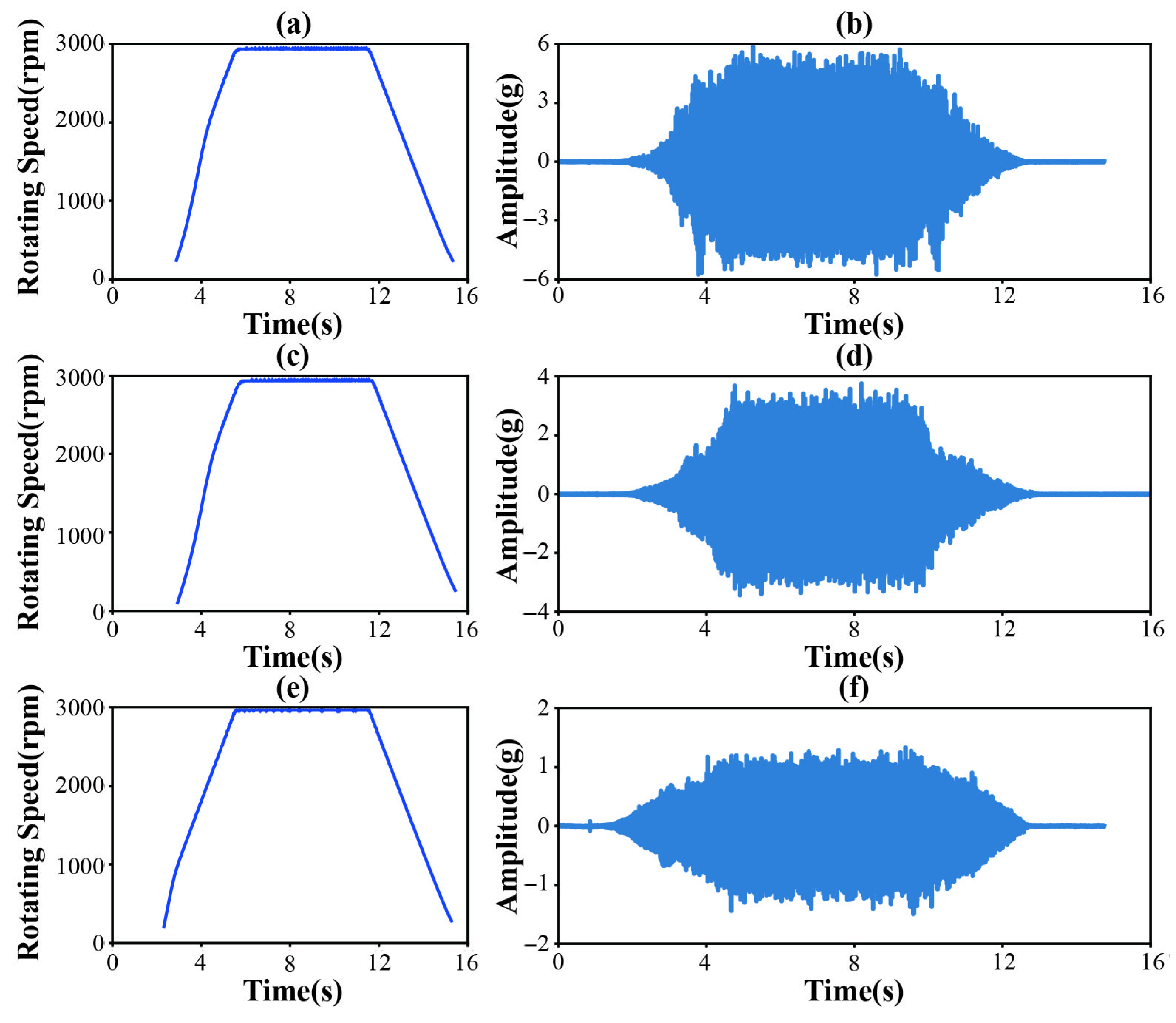
| Duration per experiment | 15 s | 0→3000→0 rpm cycle | |
| Health conditions | N, IF, OF | N: Normal; IF: Inner race fault; OF: Outer race fault | |
| Speed Profile | Acceleration rate | 200 rpm/s | Linear ramp |
| Maximum speed | 3000 rpm | 5 s dwell at maximum |
| Method | Description |
|---|---|
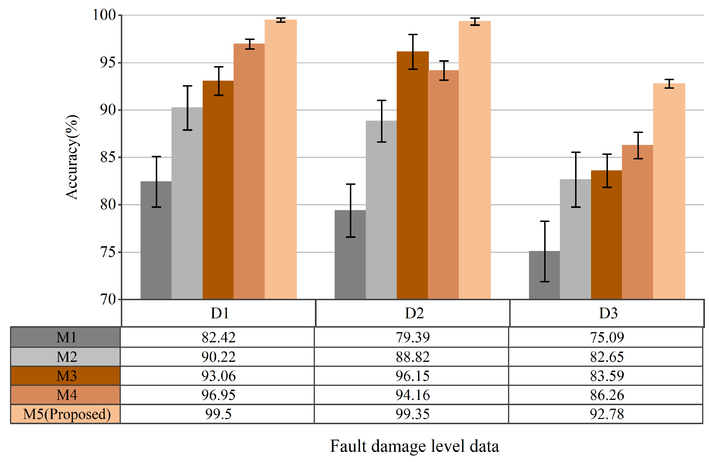
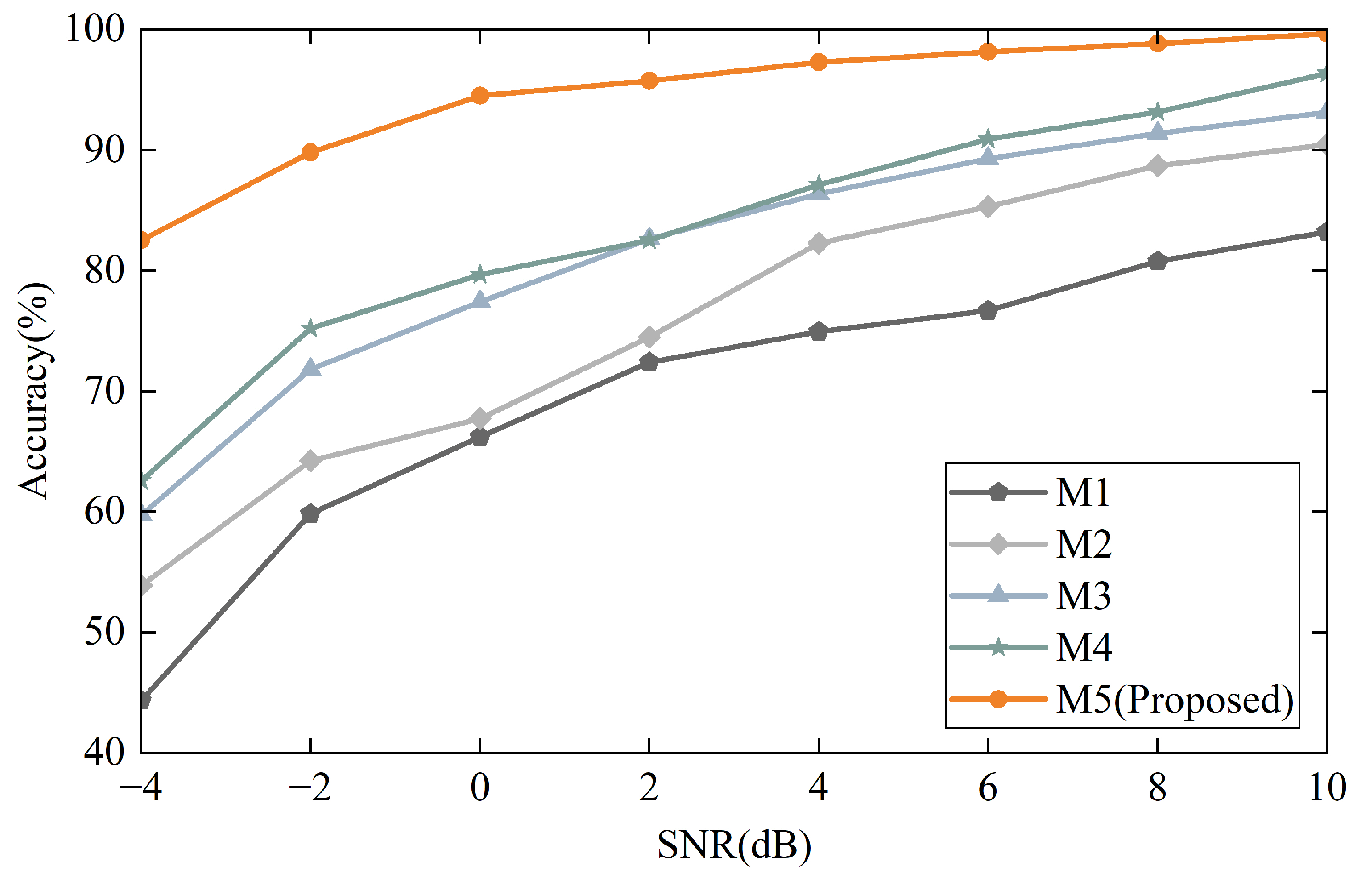
| M1 | WGWOA-VMD-SVM [15], a rolling-bearing-fault diagnosis method based on WGWOA-VMD-SVM. |
| M2 | VMD+CNN [44], a novel feature extraction and fault diagnosis method for planetary gears based on VMD, SVD, and CNN. |
| M3 | CNN-C [16], a fault diagnosis method for unknown working conditions. |
| M4 | WDCNN [20], a fault diagnosis method with noise resistance and domain Adaptation Capability. |
| M5 | VMD-AD+DWMFCNN (proposed method), a rolling-bearing-fault diagnosis method based on a dual multi-scale mechanism applicable to noise-variable operating conditions proposed in this paper. |
Disclaimer/Publisher’s Note: The statements, opinions and data contained in all publications are solely those of the individual author(s) and contributor(s) and not of MDPI and/or the editor(s). MDPI and/or the editor(s) disclaim responsibility for any injury to people or property resulting from any ideas, methods, instructions or products referred to in the content. |
© 2025 by the authors. Licensee MDPI, Basel, Switzerland. This article is an open access article distributed under the terms and conditions of the Creative Commons Attribution (CC BY) license (https://creativecommons.org/licenses/by/4.0/).
Share and Cite
Kang, J.; Wang, T.; Wei, Y.; Garba, U.H.; Tian, Y. A Rolling-Bearing-Fault Diagnosis Method Based on a Dual Multi-Scale Mechanism Applicable to Noisy-Variable Operating Conditions. Sensors 2025, 25, 4649. https://doi.org/10.3390/s25154649
Kang J, Wang T, Wei Y, Garba UH, Tian Y. A Rolling-Bearing-Fault Diagnosis Method Based on a Dual Multi-Scale Mechanism Applicable to Noisy-Variable Operating Conditions. Sensors. 2025; 25(15):4649. https://doi.org/10.3390/s25154649
Chicago/Turabian StyleKang, Jing, Taiyong Wang, Ye Wei, Usman Haladu Garba, and Ying Tian. 2025. "A Rolling-Bearing-Fault Diagnosis Method Based on a Dual Multi-Scale Mechanism Applicable to Noisy-Variable Operating Conditions" Sensors 25, no. 15: 4649. https://doi.org/10.3390/s25154649
APA StyleKang, J., Wang, T., Wei, Y., Garba, U. H., & Tian, Y. (2025). A Rolling-Bearing-Fault Diagnosis Method Based on a Dual Multi-Scale Mechanism Applicable to Noisy-Variable Operating Conditions. Sensors, 25(15), 4649. https://doi.org/10.3390/s25154649