
LCFC-Laptop: A Benchmark Dataset for Detecting Surface Defects in Consumer Electronics

 ,
,
Abstract
1. Introduction
2. Materials and Methods
2.1. LCFC-Laptop Dataset
- Scratches: Visible scratches or scuff marks on laptop surfaces.
- Collisions: Damage caused by impacts or other physical factors, such as dents or cracks.
- Plain particles: Normal surfaces with minor dust or debris, considered minor defects that affect surface appearance but not functionality.
- Dirt: Stains, fingerprints, or other forms of contamination on laptop surfaces that affect cleanliness.
- Improving defect detection accuracy: The dataset includes a diverse range of defect samples, enabling the training of models capable of accurately identifying surface defects on laptops, thereby reducing false positives and false negatives.
- Enhancing automated production line inspection: The dataset serves as essential training data for industrial automation systems, increasing detection speed and accuracy while reducing the costs and errors associated with manual inspection.
- Advancing AI applications in industry: The dataset supports the development of AI technologies in industrial contexts, particularly for product quality control and visual inspection, thereby improving overall production efficiency and quality.
- Accelerating smart manufacturing: By leveraging this dataset, manufacturers can develop more efficient automated quality control systems, further driving the digital transformation of the manufacturing industry.
2.1.1. Statistics for the Object Detection Task
2.1.2. Statistics for the Segmentation Task
2.1.3. Challenges Related to the LCFC-Laptop Dataset
- Model bias toward large-area targets: Loss functions such as cross-entropy and Dice loss are typically influenced by the number of pixels. As a result, large-area classes contribute more to the total loss, making the model more likely to learn these categories effectively. This reduces prediction accuracy for small-area targets, which may even be completely overlooked—a phenomenon known as being “overwhelmed” or “dominated by the head class”.
- Feature loss in small targets: The features of small defects, such as edges or textures, are often blurred or lost through multiple convolutional and downsampling layers in a feature pyramid, making it difficult for the model to recognize tiny abnormal regions. These issues are especially prominent in applications such as consumer electronics, where defects such as microcracks or dust particles are very small.
- Annotation sensitivity: For small-area targets, even slight annotation misalignments can cause a significant drop in the mean intersection over union (mIoU). This is particularly critical in pixel-level tasks, where high precision is required to segment small objects accurately.
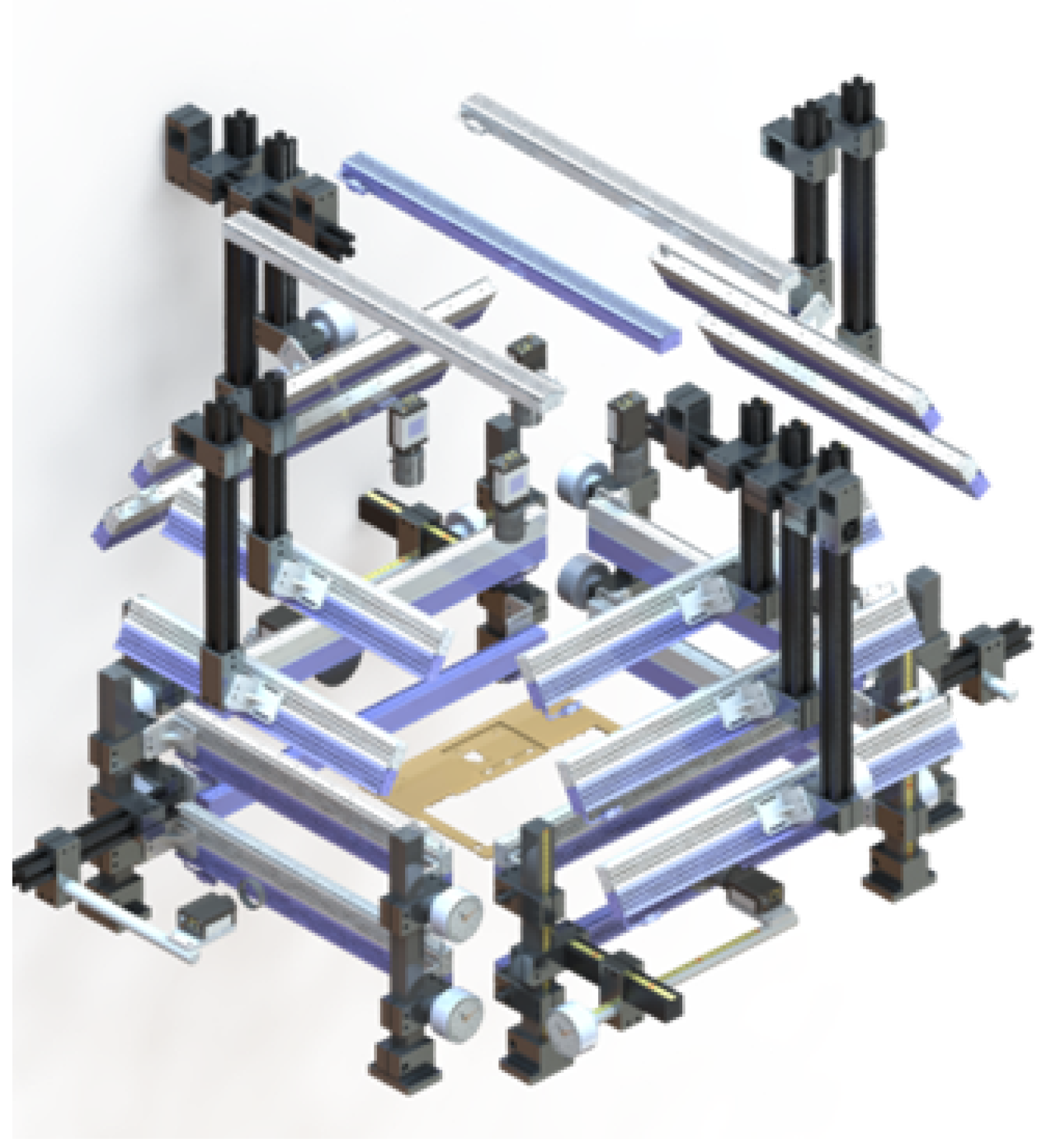
2.2. Optical Sampling System
- White light: Suitable for detecting color abnormalities but has limited resistance to ambient light interference.
- Red light: Ideal for detecting internal defects.
- Blue light: Effective for identifying microcracks and surface burrs.
2.3. Annotation of the LCFC-Laptop Dataset
2.4. Data Evaluation
2.4.1. Rationale for Using Convolution-Based Segmentation Models
2.4.2. The Selected Segmentation Models
DeepLabV3+
- Atrous (dilated) separable convolution is applied in both the atrous spatial pyramid pooling (ASPP) and decoder modules to improve computational efficiency.
- The framework allows control over the resolution of extracted features to balance model precision and computational cost.
YOLOv8-Seg
- Unified detection and segmentation: YOLOv8-Seg integrates object detection and segmentation into a single architecture. Unlike traditional segmentation models requiring separate processing pipelines, it performs bounding-box regression and mask prediction simultaneously, improving efficiency.
- Efficient architecture: YOLOv8-Seg uses a modified CSP-Darknet backbone [52], optimized for lightweight, high-speed inference processes. It employs a neck structure combining feature pyramid networks (FPNs) [53] and path-aggregation networks (PANs) [54] to enhance multiscale feature representations, increasing robustness for objects of varying sizes.
- Convolutional mask prediction: Rather than relying on transformer-based approaches, YOLOv8-Seg employs a convolutional mask prediction head, which is more computationally efficient. Segmentation masks are generated using a dynamic kernel-based approach, with each detected object assigned a segmentation kernel.
- Loss function optimization: The model uses a combination of CIoU loss [55] for bounding-box regression and binary cross-entropy loss for mask prediction, ensuring accurate localization and high-quality segmentation.
- Real-time performance: YOLOv8-Seg achieves real-time processing, making it suitable for applications such as autonomous driving, medical image analysis, video surveillance, and augmented reality.
U-Net
- High accuracy with limited data: Designed for medical imaging, where labeled data are scarce, U-Net effectively learns from small datasets using data augmentation.
- Effective use of skip connections: Unlike standard FCNs, U-Net combines low-level and high-level features to recover fine spatial details, improving boundary segmentation.
- Fully convolutional architecture: The absence of fully connected layers makes the model efficient and compatible with various input sizes.
- Fast training and inference: Its relatively simple architecture enables fast convergence and real-time inference in some applications.
FCNs
2.4.3. Experimental Design
- DeepLabV3+: Used ResNet50 as the backbone with input image dimensions of 1024 × 1024. During training, data augmentation techniques, including random resizing, cropping, and flipping, were applied using preset ratios. The model was trained using stochastic gradient descent (SGD) with a learning rate of 0.01, momentum of 0.9, and batch size of 2.
- FCN: Also used ResNet50 as the backbone, with input image dimensions of 1024 × 1024. The same data augmentation techniques—random resizing, cropping, and flipping—were applied. Training was performed using SGD with a learning rate of 0.01, momentum of 0.9, and batch size of 2.
- U-Net: Used the U-Net-S5-D16 architecture as the backbone, with an FCN head as an auxiliary head, and an input image size of 1024 × 1024. Data augmentation techniques included random resizing, cropping, and flipping. The model was trained using SGD with a learning rate of 0.01, momentum of 0.9, and batch size of 2.
- YOLOv8-Seg: Used the YOLOv8-X model as the backbone, with an input image size of 1280 × 1280. Data augmentation strategies included Mosaic augmentation, random scaling, and cropping. Training was performed using SGD with a learning rate of 0.01, momentum of 0.937, and batch size of 2.
3. Results
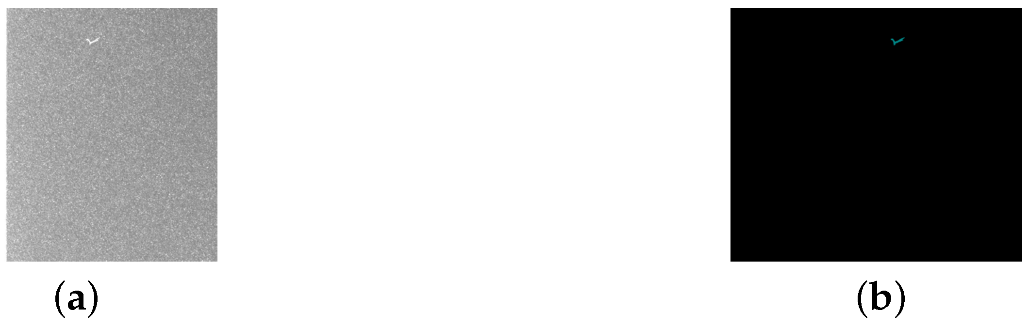
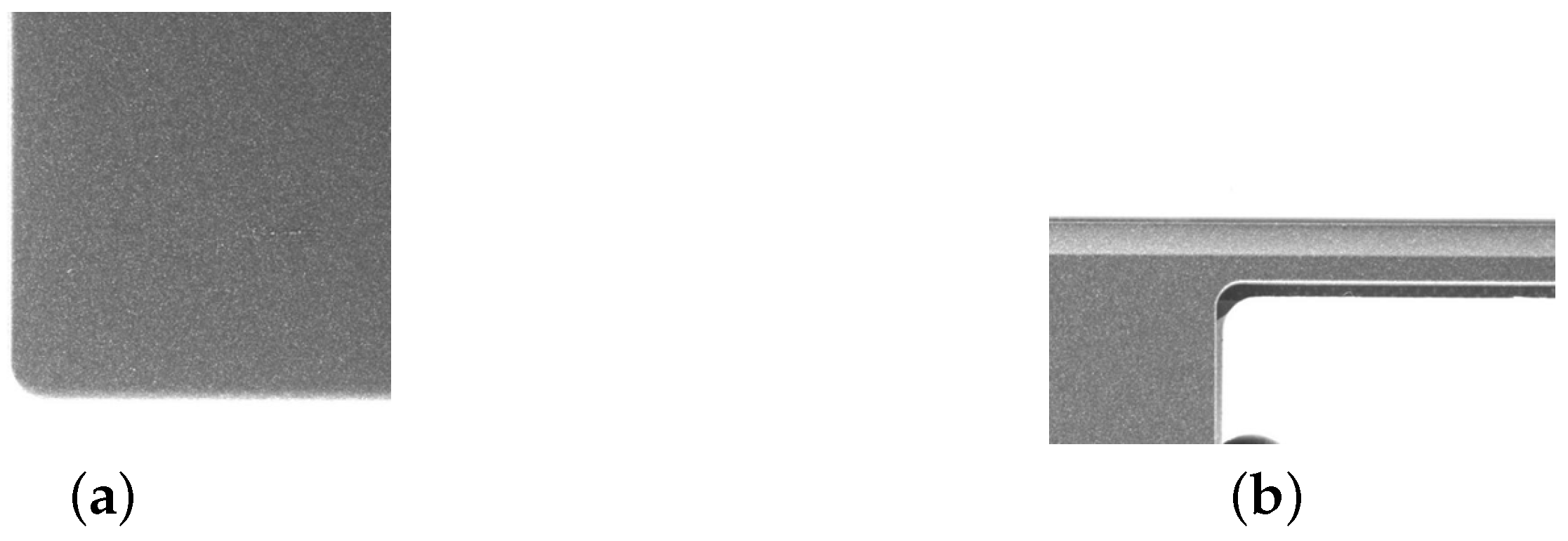
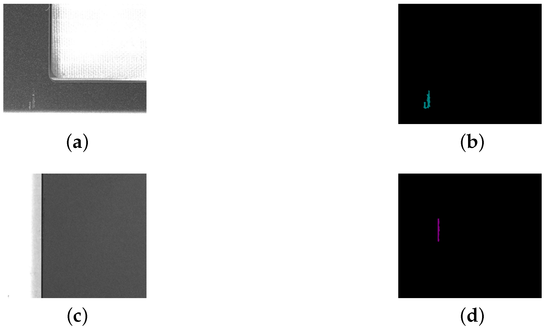
- Blurry defects: As shown in Figure 15, the contrast between defects and their backgrounds was relatively low, making them difficult to distinguish with the naked eye and often resulting in missed annotations. Segmentation models also tended to perform poorly on such low-contrast defects.
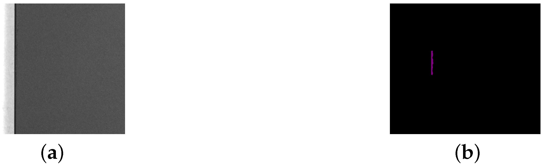
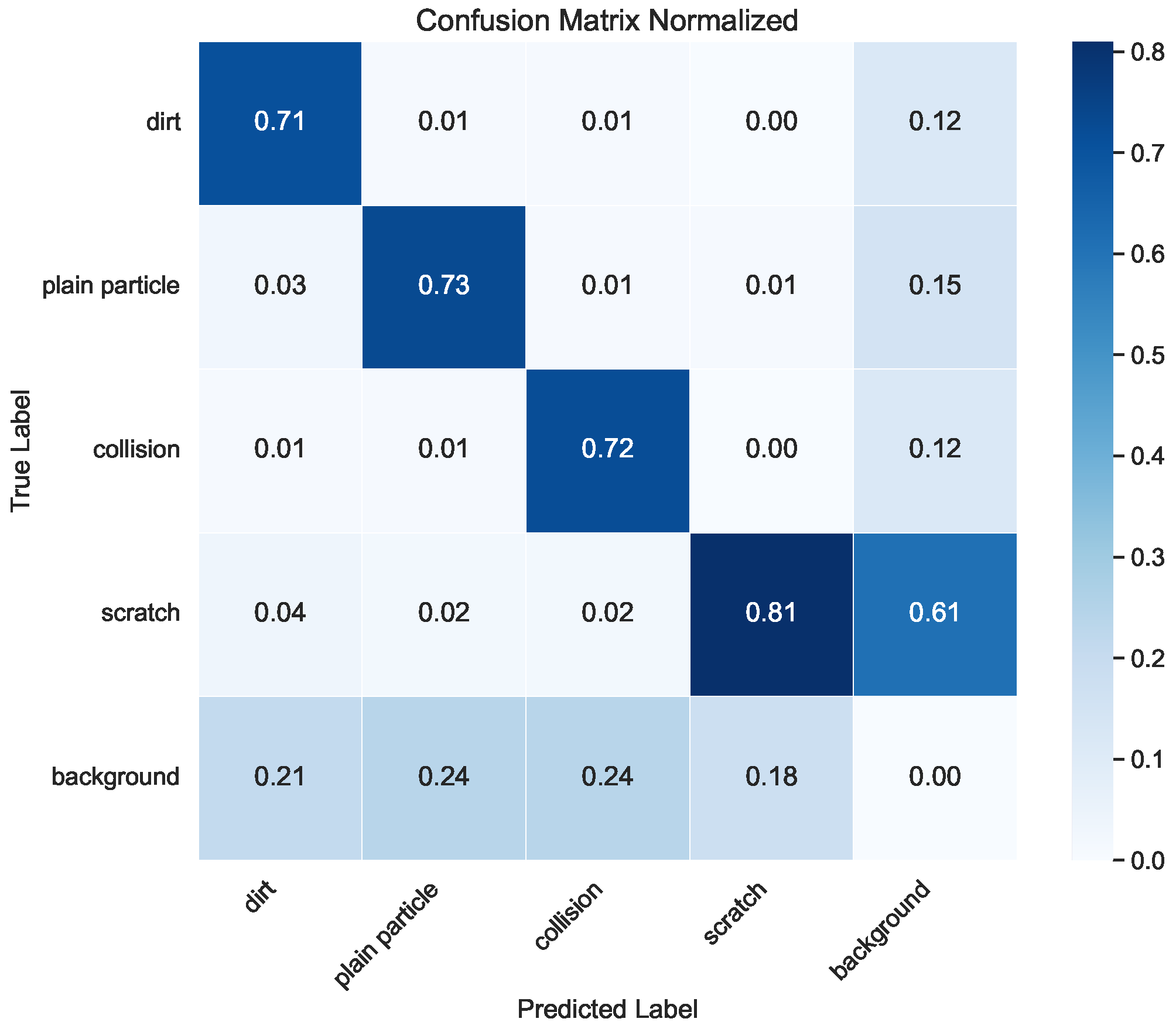
- Visual similarity between defect categories: As illustrated in Figure 16, different types of defects were visually similar, leading to frequent misclassifications. For example, thin, elongated dirt marks can closely resemble scratches, making the two difficult to distinguish.
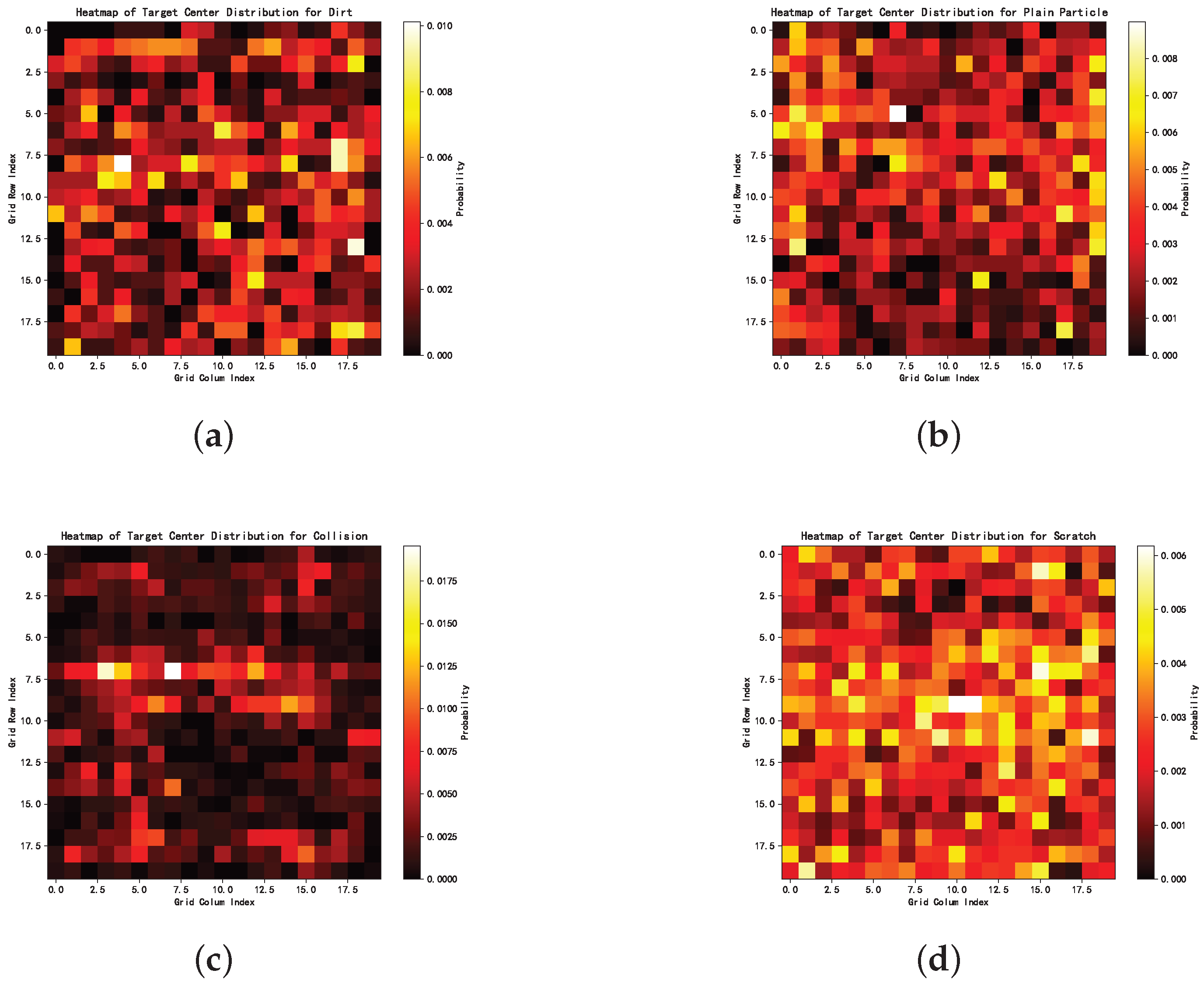
- Randomized spatial distribution: As shown in the heatmaps in Figure 17, defect locations were distributed randomly across the images, without any clear pattern. This randomness may have further increased the convergence difficulty of the networks.
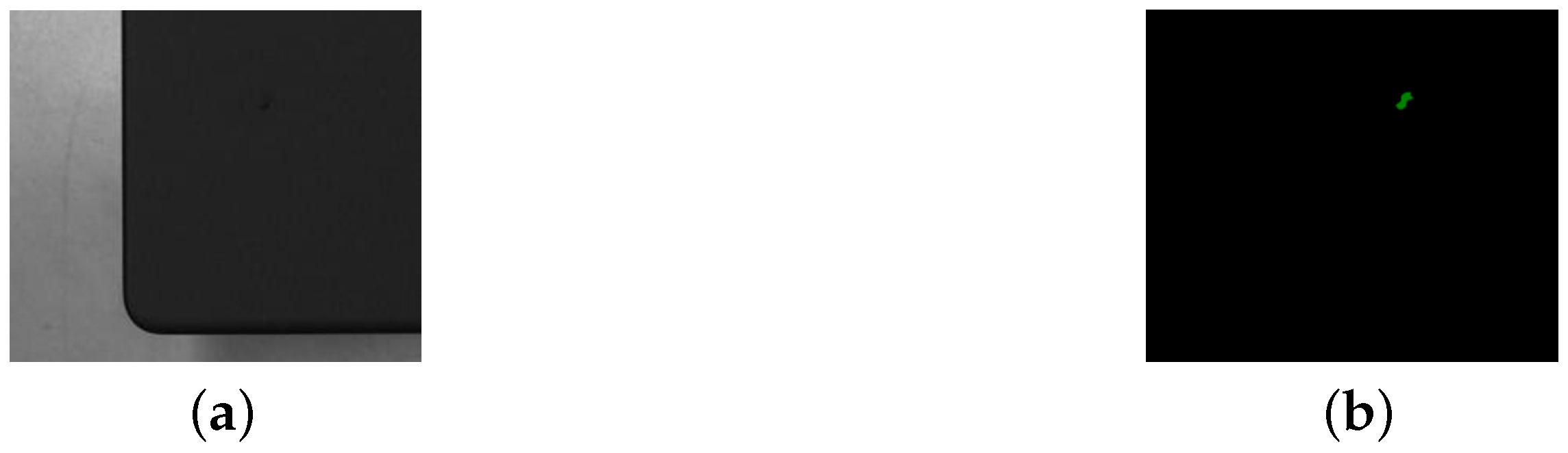
- Particle Characteristics—Defective particles are typically small, irregularly shaped objects such as dust, metal shavings, plastic debris, or coating residues. Although generally small, their shape and color may sometimes contrast with the C-cover surface, affecting visual appearance.
- Particle Location—Particles usually appear on the exposed areas of the C-cover, such as the top panel, bottom, and edges, and tend to accumulate in frequently contacted areas like corners and seams.
- Significance:
- −
- Aesthetic Degradation: The presence of particles reduces product value and compromises appearance, reducing its market appeal.
- −
- Visual Quality Impact: Particles negatively affect perceived quality. Visual imperfections may result in customer rejection, especially when appearance is a key purchasing factor.
- −
- Coating and Surface Treatment: During processes such as spraying and coating, particles can cause uneven coverage, reduced adhesion, bubbling, or peeling, thereby diminishing durability and scratch resistance.
- Significance—In production environments, the detection of particles within the acceptable tolerance range suggests that the current quality control criteria already allow for a certain degree of leniency. However, continued monitoring is essential to prevent future quality degradation. Ensuring that the frequency of such particles does not increase over time is critical to avoiding a gradual rise in defect rates that may eventually exceed acceptable limits.
4. Future Work
5. Conclusions
Author Contributions
Funding
Institutional Review Board Statement
Informed Consent Statement
Data Availability Statement
Acknowledgments
Conflicts of Interest
References
- Global Consumer Electronics Market—2024–2031. 2024. Available online: https://www.marketresearch.com/DataM-Intelligence-4Market-Research-LLP-v4207/Global-Consumer-Electronics-36170587/ (accessed on 10 July 2025).
- Zhang, T.; You, T.; Liu, Z.; Rehman, S.U.; Shi, Y.; Munshi, A. Small sample pipeline DR defect detection based on smooth variational autoencoder and enhanced detection head faster RCNN. Appl. Intell. 2025, 55, 716. [Google Scholar] [CrossRef]
- Bu, C.; Shen, R.; Bai, W.; Chen, P.; Li, R.; Zhou, R.; Li, J.; Tang, Q. CNN-based defect detection and classification of PV cells by infrared thermography method. Nondestruct. Test. Eval. 2025, 40, 1752–1769. [Google Scholar] [CrossRef]
- Hardik, J.; Patel, R.S.; Desai, H.; Vakani, H.; Mistry, M.; Dubey, N. Symptom-based early detection and classification of plant diseases using AI-driven CNN+KNN Fusion Software (ACKFS). Softw. Impacts 2025, 24, 100755. [Google Scholar] [CrossRef]
- Tareef, A. Adaptive Shape Prediction Model (ASPM) for touched and overlapping cell segmentation in cytology images. Softw. Impacts 2023, 17, 100540. [Google Scholar] [CrossRef]
- Zhou, W.; Sun, X.; Qian, X.; Fang, M. Asymmetrical Contrastive Learning Network via Knowledge Distillation for No-Service Rail Surface Defect Detection. IEEE Trans. Neural Netw. Learn. Syst. 2024, 36, 12469–12482. [Google Scholar] [CrossRef]
- Dang, T.V.; Tan, P.X. Hybrid Mobile Robot Path Planning Using Safe JBS-A*B Algorithm and Improved DWA Based on Monocular Camera. J. Intell. Robot. Syst. 2024, 110, 151. [Google Scholar] [CrossRef]
- Nascimento, R.; Ferreira, T.; Rocha, C.D.; Filipe, V.; Silva, M.F.; Veiga, G.; Rocha, L. Quality Inspection in Casting Aluminum Parts: A Machine Vision System for Filings Detection and Hole Inspection. J. Intell. Robot. Syst. 2025, 111, 53. [Google Scholar] [CrossRef]
- Małek, K.; Dybała, J.; Kordecki, A.; Hondra, P.; Kijania, K. OffRoadSynth Open Dataset for Semantic Segmentation using Synthetic-Data-Based Weight Initialization for Autonomous UGV in Off-Road Environments. J. Intell. Robot. Syst. 2024, 110, 76. [Google Scholar] [CrossRef]
- Puchalski, R.; Ha, Q.; Giernacki, W.; Nguyen, H.A.D.; Nguyen, L.V. PADRE—A Repository for Research on Fault Detection and Isolation of Unmanned Aerial Vehicle Propellers. J. Intell. Robot. Syst. 2024, 110, 74. [Google Scholar] [CrossRef]
- Wankhede, P.; Narayanaswamy, N.G.; Kurra, S.; Priyadarshini, A. SPSA: An image processing based software for single point strain analysis. Softw. Impacts 2023, 15, 100484. [Google Scholar] [CrossRef]
- Yu, N.; Wang, J.; Zhang, Z.; Han, Y.; Ding, W. Semantic Prompt Enhancement for Semi-Supervised Low-Light Salient Object Detection. IEEE Trans. Neural Netw. Learn. Syst. 2025, 36, 9933–9945. [Google Scholar] [CrossRef]
- Zhang, M.; Yue, K.; Guo, J.; Zhang, Q.; Zhang, J.; Gao, X. Computational Fluid Dynamic Network for Infrared Small Target Detection. IEEE Trans. Neural Netw. Learn. Syst. 2025. early access. [Google Scholar] [CrossRef]
- Geng, K.; Qiao, J.; Liu, N.; Yang, Z.; Zhang, R.; Li, H. Research on real-time detection of stacked objects based on deep learning. J. Intell. Robot. Syst. 2023, 109, 82. [Google Scholar] [CrossRef]
- Zheng, X.; Lin, X.; Qing, L.; Ou, X. Semantic-Aware Remote Sensing Change Detection with Multi-Scale Cross-Attention. Sensors 2025, 25, 2813. [Google Scholar] [CrossRef] [PubMed]
- Zhang, J.; Zhang, Z.; Chen, Q.; Li, G.; Li, W.; Ding, S.; Xiong, M.; Zhang, W.; Chen, S. Representation Learning Based on Co-Evolutionary Combined With Probability Distribution Optimization for Precise Defect Location. IEEE Trans. Neural Netw. Learn. Syst. 2024, 36, 11989–12003. [Google Scholar] [CrossRef] [PubMed]
- Liu, J.; Zhao, H.; Chen, Z.; Wang, Q.; Shen, X.; Zhang, H. A Dynamic Weights-Based Wavelet Attention Neural Network for Defect Detection. IEEE Trans. Neural Networks Learn. Syst. 2024, 35, 16211–16221. [Google Scholar] [CrossRef] [PubMed]
- Lin, T.Y.; Maire, M.; Belongie, S.; Hays, J.; Zitnick, C.L. Microsoft COCO: Common Objects in Context. In Computer Vision—ECCV 2014; Springer International Publishing: Berlin/Heidelberg, Germany, 2014. [Google Scholar]
- Everingham, M.; Van Gool, L.; Williams, C.K.; Winn, J.; Zisserman, A. The Pascal Visual Object Classes (VOC) Challenge. Int. J. Comput. Vis. 2010, 88, 303–338. [Google Scholar] [CrossRef]
- Bergmann, P.; Fauser, M.; Sattlegger, D.; Steger, C. MVTec AD—A Comprehensive Real-World Dataset for Unsupervised Anomaly Detection. In Proceedings of the 2019 IEEE/CVF Conference on Computer Vision and Pattern Recognition (CVPR), Long Beach, CA, USA, 15–20 June 2019; pp. 9584–9592. [Google Scholar] [CrossRef]
- Zhang, C.; Feng, S.; Wang, X.; Wang, Y. ZJU-Leaper: A Benchmark Dataset for Fabric Defect Detection and a Comparative Study. IEEE Trans. Artif. Intell. 2020, 1, 219–232. [Google Scholar] [CrossRef]
- Gao, T.; Yang, J.; Wang, W.; Fan, X. A domain feature decoupling network for rotating machinery fault diagnosis under unseen operating conditions. Reliab. Eng. Syst. Saf. 2024, 252, 110449. [Google Scholar] [CrossRef]
- Chen, Y.; Ding, Y.; Zhao, F.; Zhang, E.; Wu, Z.; Shao, L. Surface Defect Detection Methods for Industrial Products: A Review. Appl. Sci. 2021, 11, 7657. [Google Scholar] [CrossRef]
- Saberironaghi, A.; Ren, J.; El-Gindy, M. Defect Detection Methods for Industrial Products Using Deep Learning Techniques: A Review. Algorithms 2023, 16, 95. [Google Scholar] [CrossRef]
- Li, X.; Ding, H.; Yuan, H.; Zhang, W.; Pang, J.; Cheng, G.; Chen, K.; Liu, Z.; Loy, C.C. Transformer-Based Visual Segmentation: A Survey. IEEE Trans. Pattern Anal. Mach. Intell. 2024, 46, 10138–10163. [Google Scholar] [CrossRef] [PubMed]
- Xiao, H.; Li, L.; Liu, Q.; Zhu, X.; Zhang, Q. Transformers in medical image segmentation: A review. Biomed. Signal Process. Control 2023, 84, 104791. [Google Scholar] [CrossRef]
- Yao, W.; Bai, J.; Liao, W.; Chen, Y.; Liu, M.; Xie, Y. From CNN to Transformer: A Review of Medical Image Segmentation Models. J. Imaging Inform. Med. 2024, 37, 1529–1547. [Google Scholar] [CrossRef]
- Huang, X.; Deng, Z.; Li, D.; Yuan, X.; Fu, Y. MISSFormer: An Effective Transformer for 2D Medical Image Segmentation. IEEE Trans. Med. Imaging 2023, 42, 1484–1494. [Google Scholar] [CrossRef]
- Roy, S.; Koehler, G.; Ulrich, C.; Baumgartner, M.; Petersen, J.; Isensee, F.; Jäger, P.F.; Maier-Hein, K.H. MedNeXt: Transformer-Driven Scaling of ConvNets for Medical Image Segmentation. In Proceedings of the Medical Image Computing and Computer Assisted Intervention—MICCAI, Vancouver, BC, Canada, 8–12 October 2023; Greenspan, H., Madabhushi, A., Mousavi, P., Salcudean, S., Duncan, J., Syeda-Mahmood, T., Taylor, R., Eds.; Springer: Cham, Switzerland, 2023; pp. 405–415. [Google Scholar]
- Qi, Y.; He, Y.; Qi, X.; Zhang, Y.; Yang, G. Dynamic Snake Convolution based on Topological Geometric Constraints for Tubular Structure Segmentation. In Proceedings of the 2023 IEEE/CVF International Conference on Computer Vision (ICCV), Paris, France, 1–6 October 2023; pp. 6047–6056. [Google Scholar] [CrossRef]
- Yin, Y.; Han, Z.; Jian, M.; Wang, G.G.; Chen, L.; Wang, R. AMSUnet: A neural network using atrous multi-scale convolution for medical image segmentation. Comput. Biol. Med. 2023, 162, 107120. [Google Scholar] [CrossRef]
- Lei, T.; Zhang, D.; Du, X.; Wang, X.; Wan, Y.; Nandi, A.K. Semi-Supervised Medical Image Segmentation Using Adversarial Consistency Learning and Dynamic Convolution Network. IEEE Trans. Med Imaging 2023, 42, 1265–1277. [Google Scholar] [CrossRef]
- Rezvani, S.; Fateh, M.; Jalali, Y.; Fateh, A. FusionLungNet: Multi-scale fusion convolution with refinement network for lung CT image segmentation. Biomed. Signal Process. Control 2025, 107, 107858. [Google Scholar] [CrossRef]
- Gao, R. Rethinking Dilated Convolution for Real-time Semantic Segmentation. In Proceedings of the 2023 IEEE/CVF Conference on Computer Vision and Pattern Recognition Workshops (CVPRW), Vancouver, BC, Canada, 17–24 June 2023; pp. 4675–4684. [Google Scholar] [CrossRef]
- Tragakis, A.; Kaul, C.; Murray-Smith, R.; Husmeier, D. The Fully Convolutional Transformer for Medical Image Segmentation. In Proceedings of the 2023 IEEE/CVF Winter Conference on Applications of Computer Vision (WACV), Waikoloa, HI, USA, 2–7 January 2023; pp. 3649–3658. [Google Scholar] [CrossRef]
- Liang, J.; Yang, C.; Zeng, M.; Wang, X. TransConver: Transformer and convolution parallel network for developing automatic brain tumor segmentation in MRI images. Quant. Imaging Med. Surg. 2022, 12, 2397. [Google Scholar] [CrossRef]
- Dhamija, T.; Gupta, A.; Gupta, S.; Anjum; Katarya, R.; Singh, G. Semantic Segmentation in Medical Images Through Transfused Convolution and Transformer Networks. Appl. Intell. 2023, 53, 1132–1148. [Google Scholar] [CrossRef]
- Tao, H.; Liu, B.; Cui, J.; Zhang, H. A Convolutional-Transformer Network for Crack Segmentation with Boundary Awareness. In Proceedings of the 2023 IEEE International Conference on Image Processing (ICIP), Kuala Lumpur, Malaysia, 8–11 October 2023; pp. 86–90. [Google Scholar] [CrossRef]
- Cai, Y.; Long, Y.; Han, Z.; Liu, M.; Zheng, Y.; Yang, W.; Chen, L. Swin Unet3D: A Three-Dimensional Medical Image Segmentation Network Combining Vision Transformer and Convolution. BMC Med. Inform. Decis. Mak. 2023, 23, 33. [Google Scholar] [CrossRef]
- Ronneberger, O.; Fischer, P.; Brox, T. U-Net: Convolutional Networks for Biomedical Image Segmentation. In Proceedings of the Medical Image Computing and Computer-Assisted Intervention—MICCAI 2015, Munich, Germany, 5–9 October 2015; Navab, N., Hornegger, J., Wells, W.M., Frangi, A.F., Eds.; Springer: Cham, Switzerland, 2015; pp. 234–241. [Google Scholar]
- Shelhamer, E.; Long, J.; Darrell, T. Fully Convolutional Networks for Semantic Segmentation. IEEE Trans. Pattern Anal. Mach. Intell. 2017, 39, 640–651. [Google Scholar] [CrossRef]
- Chen, L.C.; Zhu, Y.; Papandreou, G.; Schroff, F.; Adam, H. Encoder-Decoder with Atrous Separable Convolution for Semantic Image Segmentation. In Proceedings of the Computer Vision—ECCV 2018, Munich, Germany, 8–14 September 2018; Ferrari, V., Hebert, M., Sminchisescu, C., Weiss, Y., Eds.; Springer: Cham, Switzerland, 2018; pp. 833–851. [Google Scholar]
- Ultralytics. YOLOv8. 2025. Available online: https://github.com/ultralytics/ultralytics (accessed on 15 July 2024).
- Redmon, J.; Divvala, S.; Girshick, R.; Farhadi, A. You Only Look Once: Unified, Real-Time Object Detection. In Proceedings of the 2016 IEEE Conference on Computer Vision and Pattern Recognition (CVPR), Los Alamitos, CA, USA, 27–30 June 2016; pp. 779–788. [Google Scholar] [CrossRef]
- Sharma, S.; Kumar, S. The Xception model: A potential feature extractor in breast cancer histology images classification. ICT Express 2022, 8, 101–108. [Google Scholar] [CrossRef]
- Chollet, F. Xception: Deep Learning with Depthwise Separable Convolutions. In Proceedings of the 2017 IEEE Conference on Computer Vision and Pattern Recognition (CVPR), Honolulu, HI, USA, 21–26 July 2017; pp. 1800–1807. [Google Scholar] [CrossRef]
- Shaheed, K.; Mao, A.; Qureshi, I.; Kumar, M.; Hussain, S.; Ullah, I.; Zhang, X. DS-CNN: A pre-trained Xception model based on depth-wise separable convolutional neural network for finger vein recognition. Expert Syst. Appl. 2022, 191, 116288. [Google Scholar] [CrossRef]
- Cordts, M.; Omran, M.; Ramos, S.; Rehfeld, T.; Enzweiler, M.; Benenson, R.; Franke, U.; Roth, S.; Schiele, B. The Cityscapes Dataset for Semantic Urban Scene Understanding. In Proceedings of the 2016 IEEE Conference on Computer Vision and Pattern Recognition (CVPR), Las Vegas, NV, USA, 27–30 June 2016; pp. 3213–3223. [Google Scholar] [CrossRef]
- Kuo, T.C.; Cheng, T.W.; Lin, C.K.; Chang, M.C.; Cheng, K.Y.; Cheng, Y.C. Using DeepLab v3+-based semantic segmentation to evaluate platelet activation. Med Biol. Eng. Comput. 2022, 60, 1775–1785. [Google Scholar] [CrossRef] [PubMed]
- Si, Y.; Gong, D.; Guo, Y.; Zhu, X.; Huang, Q.; Evans, J.; He, S.; Sun, Y. An Advanced Spectral–Spatial Classification Framework for Hyperspectral Imagery Based on DeepLab v3+. Appl. Sci. 2021, 11, 5703. [Google Scholar] [CrossRef]
- Chen, H.; Qin, Y.; Liu, X.; Wang, H.; Zhao, J. An improved DeepLabv3+ lightweight network for remote-sensing image semantic segmentation. Complex Intell. Syst. 2024, 10, 2839–2849. [Google Scholar] [CrossRef]
- Bochkovskiy, A.; Wang, C.Y.; Liao, H.Y.M. YOLOv4: Optimal Speed and Accuracy of Object Detection. arXiv 2020, arXiv:2004.10934. [Google Scholar] [CrossRef]
- Lin, T.Y.; Dollár, P.; Girshick, R.; He, K.; Hariharan, B.; Belongie, S. Feature Pyramid Networks for Object Detection. In Proceedings of the 2017 IEEE Conference on Computer Vision and Pattern Recognition (CVPR), Honolulu, HI, USA, 21–26 July 2017; pp. 936–944. [Google Scholar] [CrossRef]
- Liu, S.; Qi, L.; Qin, H.; Shi, J.; Jia, J. Path Aggregation Network for Instance Segmentation. In Proceedings of the 2018 IEEE/CVF Conference on Computer Vision and Pattern Recognition, Salt Lake City, UT, USA, 18–23 June 2018; pp. 8759–8768. [Google Scholar] [CrossRef]
- Zheng, Z.; Wang, P.; Liu, W.; Li, J.; Ye, R.; Ren, D. Distance-IoU Loss: Faster and Better Learning for Bounding Box Regression. arXiv 2019, arXiv:1911.08287. [Google Scholar] [CrossRef]
- Wang, H.; Wang, G.; Li, Y.; Zhang, K. YOLO-HV: A fast YOLOv8-based method for measuring hemorrhage volumes. Biomed. Signal Process. Control 2025, 100, 107131. [Google Scholar] [CrossRef]
- Hua, Y.; Chen, R.; Qin, H. YOLO-DentSeg: A Lightweight Real-Time Model for Accurate Detection and Segmentation of Oral Diseases in Panoramic Radiographs. Electronics 2025, 14, 805. [Google Scholar] [CrossRef]
- AlSubaie, N.A.; AlMalki, G.A.; AlMutairi, G.N.; AlRumaih, S.A. Road Infrastructure Defect Detection using Yolo8Seg Based Approach. In Proceedings of the 2025 IEEE 6th International Conference on Image Processing, Applications and Systems (IPAS), Lyon, France, 9–11 January 2025; Volume CFP2540Z-ART, pp. 1–6. [Google Scholar] [CrossRef]
- He, K.; Gkioxari, G.; Dollár, P.; Girshick, R. Mask R-CNN. IEEE Trans. Pattern Anal. Mach. Intell. 2020, 42, 386–397. [Google Scholar] [CrossRef]
- Azad, R.; Aghdam, E.K.; Rauland, A.; Jia, Y.; Avval, A.H.; Bozorgpour, A.; Karimijafarbigloo, S.; Cohen, J.P.; Adeli, E.; Merhof, D. Medical Image Segmentation Review: The Success of U-Net. IEEE Trans. Pattern Anal. Mach. Intell. 2024, 46, 10076–10095. [Google Scholar] [CrossRef]
- Zhang, S.; Zhang, C. Modified U-Net for plant diseased leaf image segmentation. Comput. Electron. Agric. 2023, 204, 107511. [Google Scholar] [CrossRef]
- Williams, C.; Falck, F.; Deligiannidis, G.; Holmes, C.; Doucet, A.; Syed, S. A unified framework for U-net design and analysis. In Proceedings of the 37th International Conference on Neural Information Processing Systems, Red Hook, NY, USA, 10–16 December 2023. NIPS ’23. [Google Scholar]
- Yu, Z.; Yu, L.; Zheng, W.; Wang, S. EIU-Net: Enhanced feature extraction and improved skip connections in U-Net for skin lesion segmentation. Comput. Biol. Med. 2023, 162, 107081. [Google Scholar] [CrossRef] [PubMed]
- M. Gab Allah, A.; M. Sarhan, A.; M. Elshennawy, N. Edge U-Net: Brain tumor segmentation using MRI based on deep U-Net model with boundary information. Expert Syst. Appl. 2023, 213, 118833. [Google Scholar] [CrossRef]
- Kotwal, J.; Kashyap, R.; Shafi, P.M.; Kimbahune, V. Enhanced leaf disease detection: UNet for segmentation and optimized EfficientNet for disease classification. Softw. Impacts 2024, 22, 100701. [Google Scholar] [CrossRef]
- Cui, H.; Xing, T.; Ren, J.; Chen, Y.; Yu, Z.; Guo, B.; Guo, X. eSwin-UNet: A Collaborative Model for Industrial Surface Defect Detection. In Proceedings of the 2022 IEEE 28th International Conference on Parallel and Distributed Systems (ICPADS), Nanjing, China, 10–12 January 2023; pp. 379–386. [Google Scholar] [CrossRef]
- Wong, V.W.H.; Ferguson, M.; Law, K.H.; Lee, Y.T.T.; Witherell, P. Segmentation of Additive Manufacturing Defects Using U-Net. J. Comput. Inf. Sci. Eng. 2021, 22, 031005. [Google Scholar] [CrossRef]
- Vasquez, J.; Furuhata, T.; Shimada, K. Image-Enhanced U-Net: Optimizing Defect Detection in Window Frames for Construction Quality Inspection. Buildings 2024, 14, 3. [Google Scholar] [CrossRef]
- Damacharla, P.; Achuth Rao, M.V.; Ringenberg, J.; Javaid, A.Y. TLU-Net: A Deep Learning Approach for Automatic Steel Surface Defect Detection. In Proceedings of the 2021 International Conference on Applied Artificial Intelligence (ICAPAI), Halden, Norway, 19–21 May 2021; pp. 1–6. [Google Scholar] [CrossRef]
- Zhao, H.; Liang, M.; Li, H. Research on gesture segmentation method based on FCN combined with CBAM-ResNet50. Signal Image Video Process. 2024, 18, 7729–7740. [Google Scholar] [CrossRef]


| LCFC-Laptop | MVTec AD | |
|---|---|---|
| Number of defects | 14,478 | 5354 |
| Number of lighting sources | 6 | 1 |
| Application | Surface defect detection in consumer electronics | Industrial defect detection |
| Annotation | Pixel-precise ground truth, object detection | Pixel-precise ground truth |
| Evaluation | Yes | Yes |
| Original resolution | 50005000 | 700700–10241024 |
| Defect Type | Number of Defects |
|---|---|
| Dirt | 11,285 |
| Plain particles | 605 |
| Edge particles | 35 |
| Collisions | 29 |
| Scratches | 1104 |
| Unknown | 1420 |
| All | 14,478 |
| Defect Type | Number of Defects |
|---|---|
| Dirt | 2572 |
| Plain particles | 4788 |
| Collisions | 5265 |
| Scratches | 9868 |
| All | 22,512 |
| Color | Model | Angle (°) |
|---|---|---|
| White | M132 | 0 |
| Blue | M133 | 0 |
| White | M134 | 0 |
| White | M123 | 30 |
| Blue | M124 | 30 |
| White | M125 | 45 |
| Blue | M126 | 45 |
| White | M127 | 60 |
| Blue | M128 | 60 |
| White | M129 | 90 |
| Blue | M130 | 90 |
| Blue | M131 | 90 |
| White | M100 | 30 |
| Blue | M101 | 30 |
| White | M102 | 45 |
| Blue | M103 | 45 |
| White | M105 | 90 |
| Blue | M106 | 90 |
| White | M106 | 90 |
| Blue | M107 | 90 |
| White | M108 | 30 |
| Blue | M109 | 30 |
| White | M110 | 45 |
| Blue | M111 | 45 |
| White | M112 | 90 |
| Blue | M113 | 90 |
| Blue | M114 | 90 |
| White | M115 | 30 |
| Blue | M116 | 30 |
| White | M117 | 45 |
| Blue | M118 | 45 |
| White | M119 | 45 |
| White | M120 | 90 |
| Blue | M121 | 90 |
| Blue | M122 | 90 |
| Wavelength (nm) | Brightness (Luminous Flux) | |
|---|---|---|
| White | Red 620–630 nm U +Blue 465–475 nm U +Green 520–530 nm | 0–130,000 |
| Red | 620–630 nm | 0–130,000 |
| Blue | 465–475 nm | 0–130,000 |
| Model | Accuracy (mAP@50 on COCO) | Inference Speed (FPS on RTX 3090) | Computational Complexity |
|---|---|---|---|
| FCN | 30+ FPS | Low | |
| DeepLabV3+ | 10–20 FPS | High | |
| U-Net | 15–25 FPS | Medium | |
| YOLOv8-Seg | 50+ FPS | Low–Medium |
| Model | Strengths | Weaknesses |
|---|---|---|
| FCN | - Simple and efficient - Works with variable input sizes - End-to-end trainable | - Lower segmentation accuracy - Lacks fine-grained details |
| DeepLabV3+ | - High segmentation accuracy - Strong boundary preservation - Performs well on complex datasets | - Slow inference speed - High computational cost |
| U-Net | - Suitable for medical and industrial segmentation - Strong boundary refinement - Performs well on small datasets | - High memory consumption - Not optimized for real-time use |
| YOLOv8-Seg | - Real-time performance - Combines object detection and segmentation - Efficient on edge devices | - Lower accuracy than DeepLabV3+ and U-Net - May struggle with fine-grained segmentation |
| Model | Batch Size | Epochs | Learning Rate | Optimizer |
|---|---|---|---|---|
| YOLOv8-Seg | 2 | 100 | 0.01 | SGD |
| Mask R-CNN | 2 | 100 | 0.01 | SGD |
| DeepLabV3+ | 2 | 100 | 0.01 | SGD |
| U-Net | 2 | 100 | 0.01 | SGD |
| YOLOv8-Seg | DeepLabV3+ | FCN | U-Net | |
|---|---|---|---|---|
| Number of parameters | 11.78 M | 41.22 M | 47.13 M | 28.99 M |
| FLOPs | 0.04 T | 0.71 T | 0.79 T | 0.81 T |
| IoU (dirt) | 0.74 | 0.50 | 0.59 | 0.42 |
| IoU (plain particles) | 0.83 | 0.49 | 0.61 | 0.41 |
| IoU (collisions) | 0.58 | 0.52 | 0.60 | 0.41 |
| IoU (scratches) | 0.77 | 0.52 | 0.59 | 0.41 |
| mIoU | 0.73 | 0.51 | 0.60 | 0.41 |
| YOLOv8-Seg | DeepLabV3+ | FCN | U-Net | |
|---|---|---|---|---|
| Number of parameters | 11.78 M | 41.22 M | 47.13 M | 28.99 M |
| FLOPs | 0.04 T | 0.71 T | 0.79 T | 0.81 T |
| IoU (dirt) | 0.62 | 0.56 | 0.61 | 0.46 |
| IoU (plain particles) | 0.66 | 0.52 | 0.61 | 0.47 |
| IoU (collisions) | 0.60 | 0.49 | 0.60 | 0.47 |
| IoU (scratches) | 0.67 | 0.53 | 0.63 | 0.46 |
| mIoU | 0.64 | 0.52 | 0.61 | 0.46 |
| YOLOv8-Seg | DeepLabV3+ | FCN | U-Net | |
|---|---|---|---|---|
| Number of parameters | 11.78 M | 41.22 M | 47.13 M | 28.99 M |
| FLOPs | 0.04 T | 0.71 T | 0.79 T | 0.81 T |
| IoU (dirt) | 0.60 | 0.52 | 0.59 | 0.41 |
| IoU (plain particles) | 0.62 | 0.49 | 0.58 | 0.40 |
| IoU (collisions) | 0.49 | 0.53 | 0.60 | 0.40 |
| IoU (scratches) | 0.68 | 0.52 | 0.59 | 0.41 |
| mIoU | 0.60 | 0.52 | 0.59 | 0.41 |
| Epoch | Learning Rate | Optimizer | mIoU |
|---|---|---|---|
| 150 | 0.01 | SGD | 0.597 |
| 150 | 0.02 | SGD | 0.751 |
| 100 | 0.01 | SGD | 0.704 |
| 150 | 0.01 | Adam | failed to converge |
| 100 | 0.02 | SGD | 0.763 |
| 100 | 0.01 | Adam | failed to converge |
| 150 | 0.02 | Adam | failed to converge |
| 100 | 0.02 | Adam | failed to converge |
| Precision | Recall | |
|---|---|---|
| Dirt | 0.716 | 0.677 |
| Plain particles | 0.717 | 0.614 |
| Collisions | 0.706 | 0.599 |
| Scratches | 0.769 | 0.769 |
| U-Net | YOLOv8-Seg | |
|---|---|---|
| Clear | 0.413 | 0.751 |
| Mildly blurred | 0.399 | 0.732 |
| Heavily blurred | 0.379 | 0.691 |
| mIoU | |
|---|---|
| Without unknown samples | 73.4% |
| With unknown samples | 70.6% |
| mIoU | |
|---|---|
| FPN | 73.2% |
| PAN | 65.6% |
| PAN+FPN | 78.4% |
| mIoU | |
|---|---|
| Backbone with attention | 71.2% |
| Backbone without attention | 70.6% |
| mIoU | |
|---|---|
| Baseline | 78.4% |
| −20% brightness | 78.7% |
| −40% brightness | 78.1% |
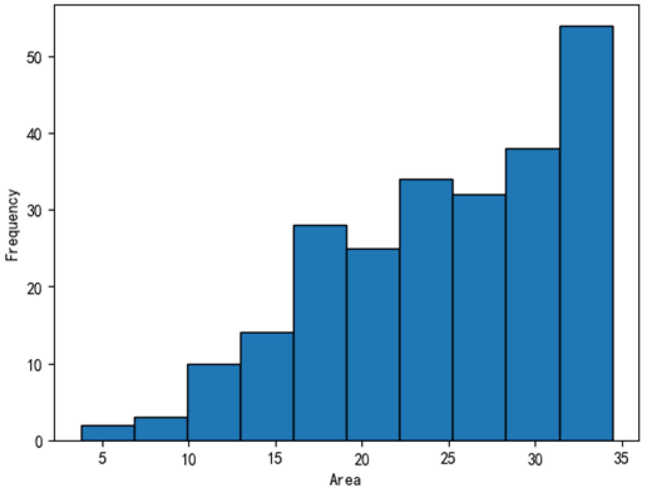
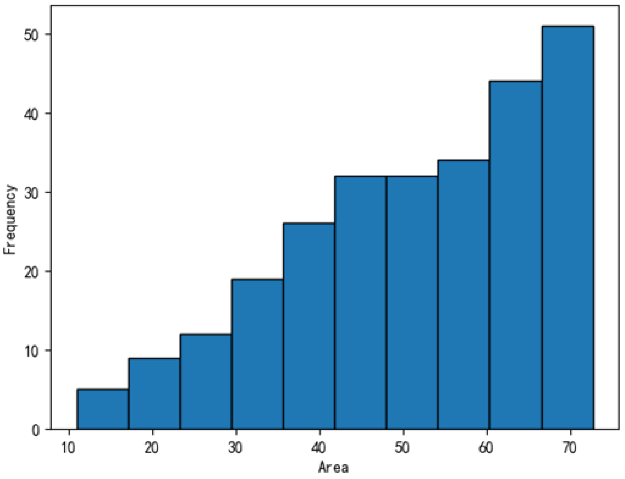
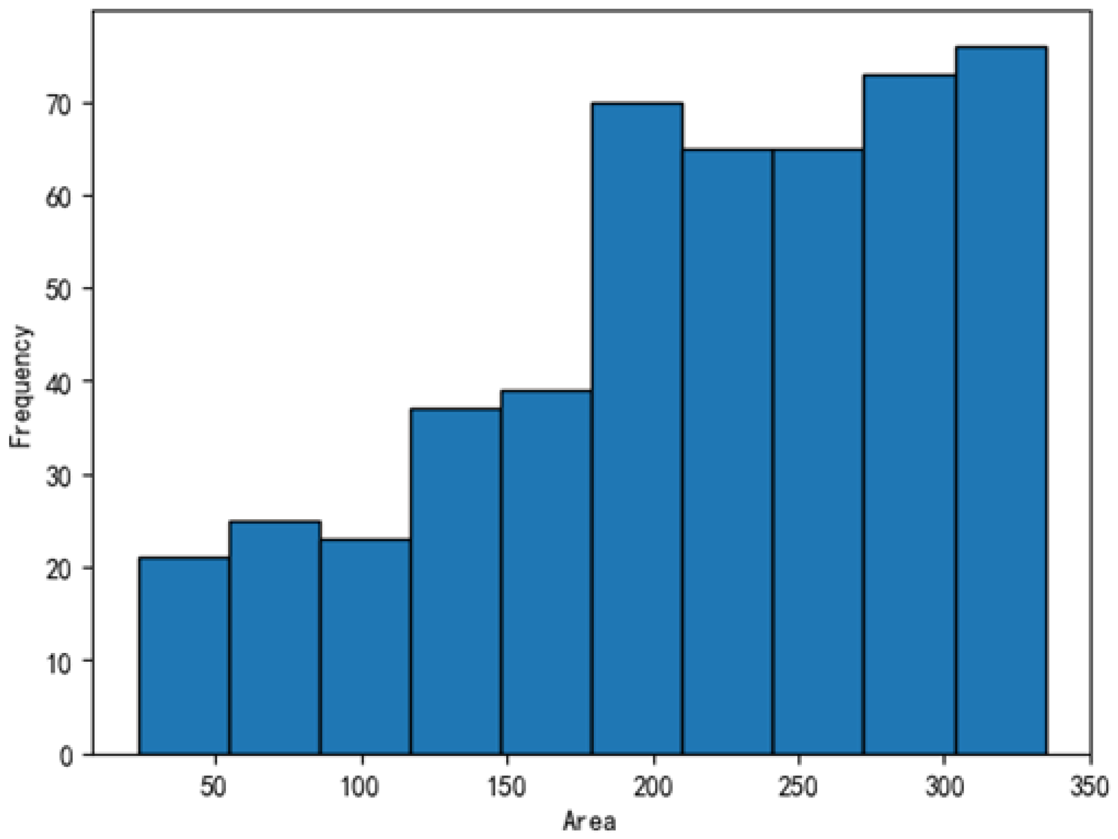
| Plain Particles | Collisions | Dirt | Scratches | |
|---|---|---|---|---|
| Mean area (pixels2) | 251.65 | 679.86 | 5101.20 | 1867.24 |
| Standard deviation of area (pixels2) | 411.05 | 61,205.08 | 67,441.41 | 2848.38 |
| Plain Particles | Collisions | Dirt | Scratches | |
|---|---|---|---|---|
| Mean perimeter (pixels) | 58.40 | 118.45 | 332.87 | 299.52 |
| Standard deviation of perimeter (pixels) | 42.42 | 98.13 | 241.24 | 177.77 |
| Plain Particles | Collisions | Dirt | Scratches | |
|---|---|---|---|---|
| Mean defect length (pixels) | 16.09 | 41.15 | 147.07 | 118.18 |
| Standard deviation of defect length (pixels) | 25.20 | 49.71 | 131.23 | 82.91 |
Disclaimer/Publisher’s Note: The statements, opinions and data contained in all publications are solely those of the individual author(s) and contributor(s) and not of MDPI and/or the editor(s). MDPI and/or the editor(s) disclaim responsibility for any injury to people or property resulting from any ideas, methods, instructions or products referred to in the content. |
© 2025 by the authors. Licensee MDPI, Basel, Switzerland. This article is an open access article distributed under the terms and conditions of the Creative Commons Attribution (CC BY) license (https://creativecommons.org/licenses/by/4.0/).
Share and Cite
Dai, H.-F.; Wang, J.-R.; Zhong, Q.; Qin, D.; Liu, H.; Guo, F. LCFC-Laptop: A Benchmark Dataset for Detecting Surface Defects in Consumer Electronics. Sensors 2025, 25, 4535. https://doi.org/10.3390/s25154535
Dai H-F, Wang J-R, Zhong Q, Qin D, Liu H, Guo F. LCFC-Laptop: A Benchmark Dataset for Detecting Surface Defects in Consumer Electronics. Sensors. 2025; 25(15):4535. https://doi.org/10.3390/s25154535
Chicago/Turabian StyleDai, Hua-Feng, Jyun-Rong Wang, Quan Zhong, Dong Qin, Hao Liu, and Fei Guo. 2025. "LCFC-Laptop: A Benchmark Dataset for Detecting Surface Defects in Consumer Electronics" Sensors 25, no. 15: 4535. https://doi.org/10.3390/s25154535
APA StyleDai, H.-F., Wang, J.-R., Zhong, Q., Qin, D., Liu, H., & Guo, F. (2025). LCFC-Laptop: A Benchmark Dataset for Detecting Surface Defects in Consumer Electronics. Sensors, 25(15), 4535. https://doi.org/10.3390/s25154535