
Masks-to-Skeleton: Multi-View Mask-Based Tree Skeleton Extraction with 3D Gaussian Splatting


Abstract
1. Introduction
2. Related Work
2.1. Three-Dimensional Tree Skeleton Extraction
2.1.1. Particle-Flow Modeling
2.1.2. Geometry-Based Methods
2.1.3. Learning-Based Methods
2.2. Image-Guided 3D Structure Reconstruction via Differentiable Rendering
3. Method
3.1. Preprocessing and Initialization
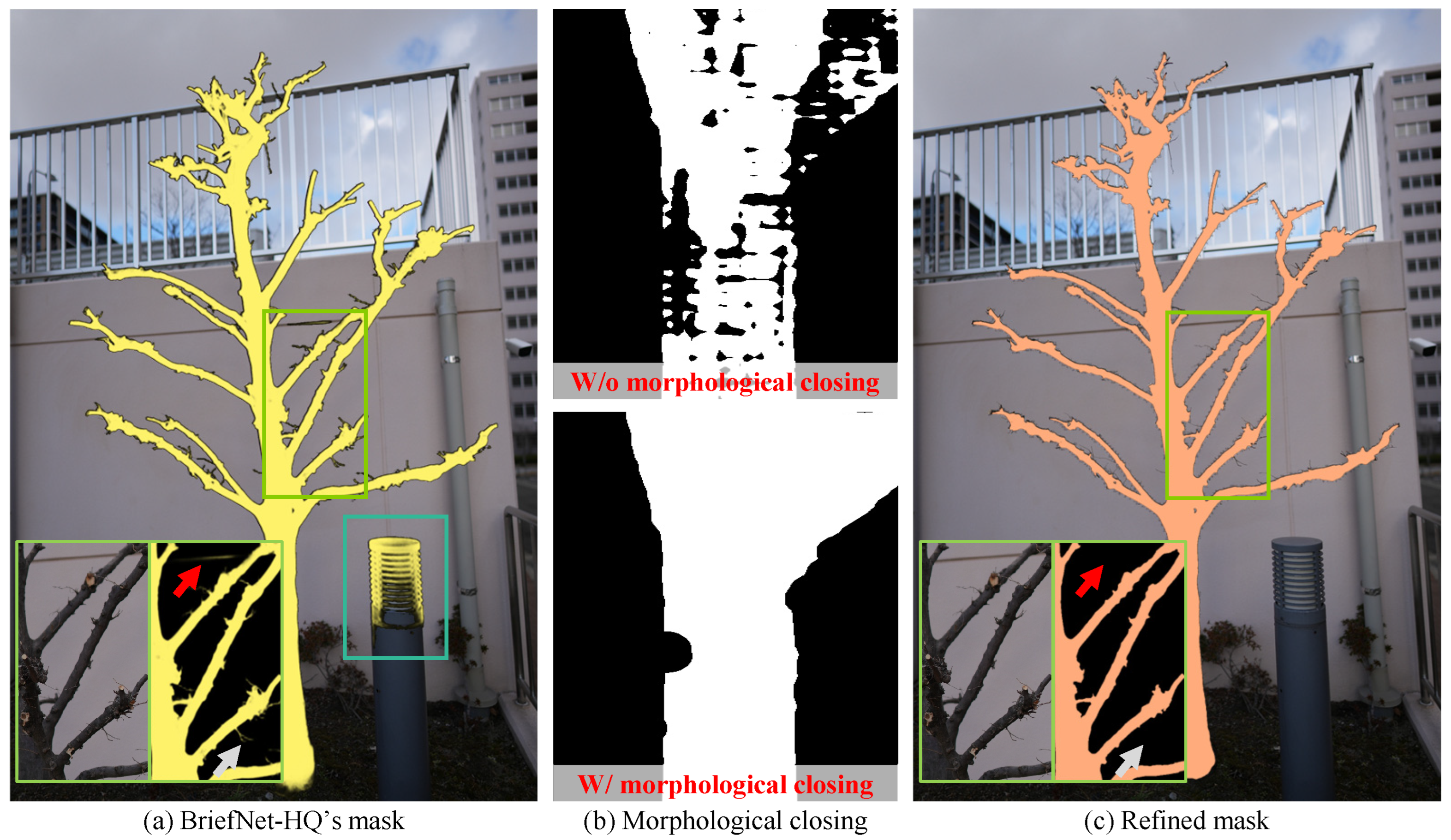
3.1.1. Mask Extraction
3.1.2. Graph Initialization
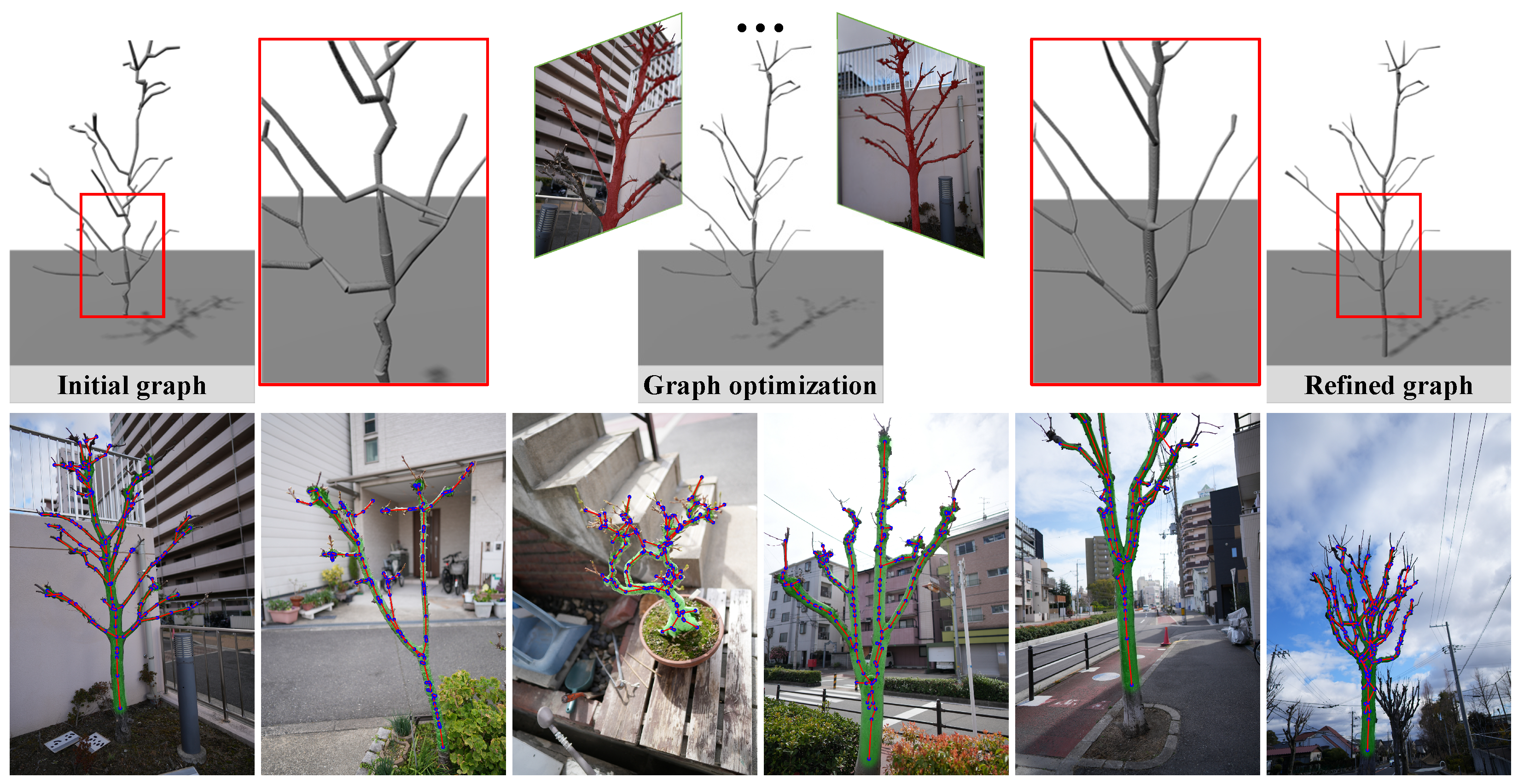
3.2. Mask-Guided Graph Refinement
3.2.1. Three-Dimensional Gaussian Splatting
3.2.2. Mask-Guided Graph Refinement
3.3. Structure-Aware Graph Optimization
3.3.1. Silhouette Supervision
3.3.2. Graph Geometry Regularization
Repulsion Loss
Edge Length Loss
Angle Fold Loss
Midpoint Direction Loss
Radius Lower Bound Loss
3.4. Overall Algorithm
| Algorithm 1: Mask-Guided Tree Skeleton Reconstruction. |
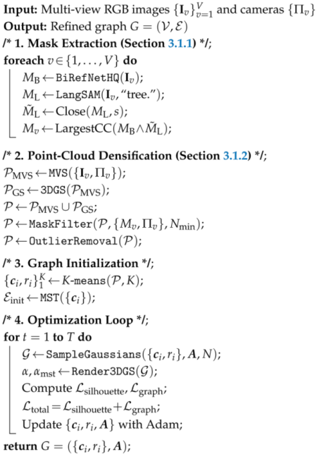 |
4. Experiments
4.1. Implementation Details
Hyper-Parameters
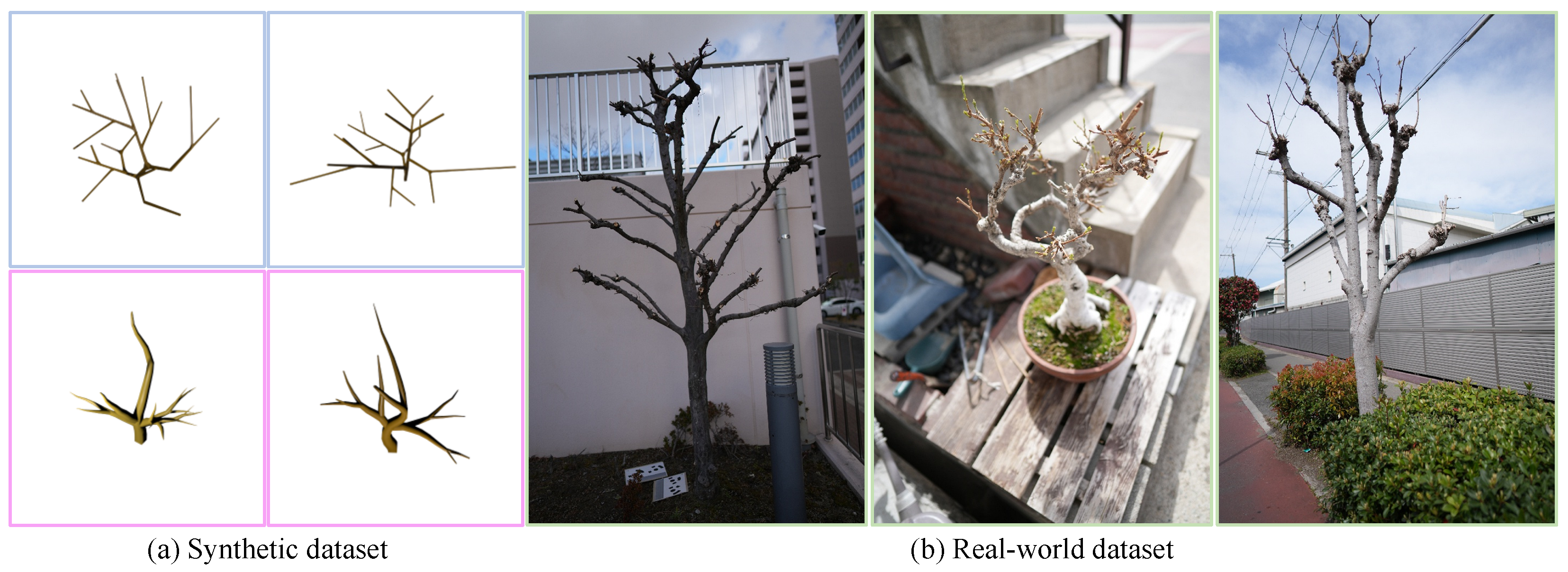
4.2. Dataset
4.3. Evaluation Metrics
4.3.1. Chamfer Distance
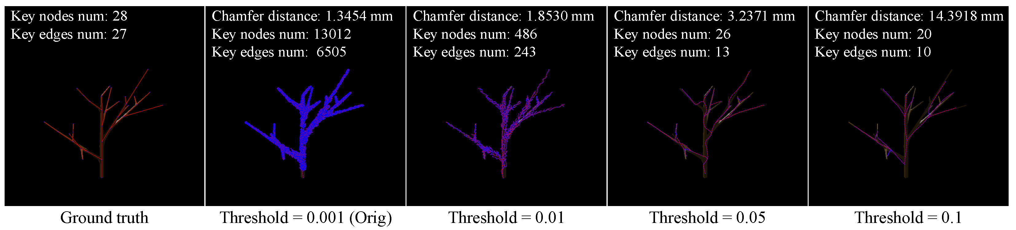
4.3.2. Node and Edge Count
4.3.3. Tree Rate
4.4. Baselines
4.4.1. adTree
4.4.2. Smart-Tree
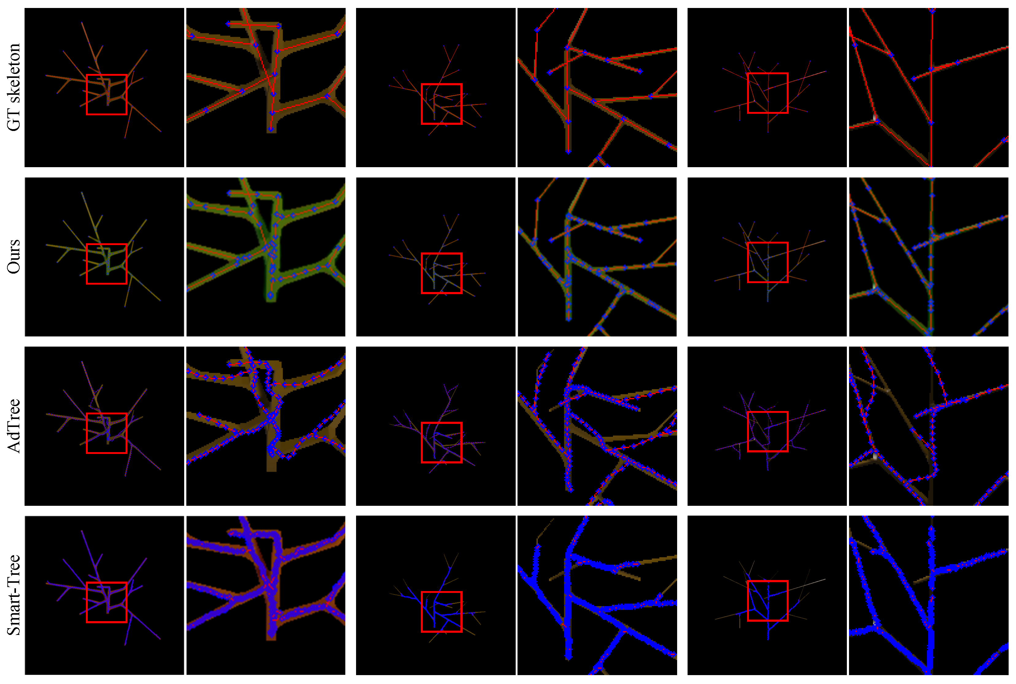
4.5. Results on the Synthetic Dataset
4.5.1. L-System-Based Dataset
4.5.2. Mtree Dataset
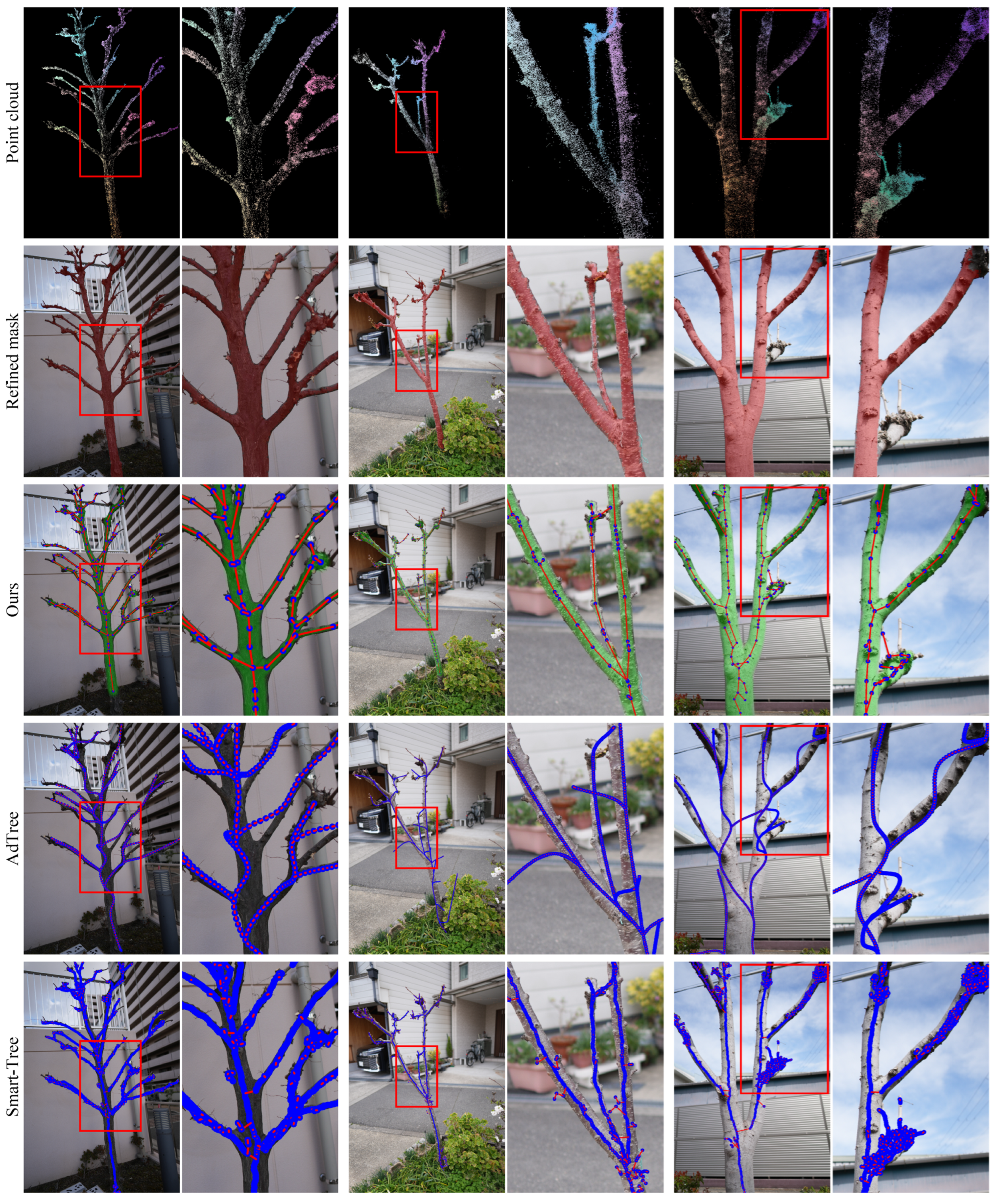
4.6. Results on the Real-World Dataset
4.7. Ablation Study
4.7.1. Without Geometry Regularization ()
4.7.2. Without an SFS Layer
4.7.3. Without an SFS Layer and Geometry Regularization
5. Conclusions
Limitations and Future Work
Author Contributions
Funding
Data Availability Statement
Conflicts of Interest
References
- Chaudhury, A.; Godin, C. Skeletonization of plant point cloud data using stochastic optimization framework. Front. Plant Sci. 2020, 11, 773. [Google Scholar] [CrossRef]
- Gentilhomme, T.; Villamizar, M.; Corre, J.; Odobez, J.M. Towards smart pruning: ViNet, a deep-learning approach for grapevine structure estimation. Comput. Electron. Agric. 2023, 207, 107736. [Google Scholar] [CrossRef]
- Cabrera-Bosquet, L.; Fournier, C.; Brichet, N.; Welcker, C.; Suard, B.; Tardieu, F. High-throughput estimation of incident light, light interception and radiation-use efficiency of thousands of plants in a phenotyping platform. New Phytol. 2016, 212, 269–281. [Google Scholar] [CrossRef]
- Sheng, W.; Wen, W.; Xiao, B.; Guo, X.; Du, J.J.; Wang, C.; Wang, Y. An accurate skeleton extraction approach from 3D point clouds of maize plants. Front. Plant Sci. 2019, 10, 248. [Google Scholar] [CrossRef]
- Fan, G.; Nan, L.; Chen, F.; Dong, Y.; Wang, Z.; Li, H.; Chen, D. A new quantitative approach to tree attributes estimation based on LiDAR point clouds. Remote Sens. 2020, 12, 1779. [Google Scholar] [CrossRef]
- Kankare, V.; Holopainen, M.; Vastaranta, M.; Puttonen, E.; Yu, X.; Hyyppä, J.; Vaaja, M.; Hyyppä, H.; Alho, P. Individual tree biomass estimation using terrestrial laser scanning. ISPRS J. Photogramm. Remote Sens. 2013, 75, 64–75. [Google Scholar] [CrossRef]
- Gaillard, M.; Miao, C.; Schnable, J.; Benes, B. Sorghum segmentation by skeleton extraction. In Proceedings of the European Conference on Computer Vision (ECCV) Workshops, Online, 23–28 August 2020; pp. 296–311. [Google Scholar] [CrossRef]
- Miao, T.; Zhu, C.; Xu, T.; Yang, T.; Li, N.; Zhou, Y.; Deng, H. Automatic stem-leaf segmentation of maize shoots using three-dimensional point cloud. Comput. Electron. Agric. 2021, 187, 106310. [Google Scholar] [CrossRef]
- Arikapudi, R.; Vougioukas, S. Robotic Tree-fruit harvesting with arrays of Cartesian Arms: A study of fruit pick cycle times. Comput. Electron. Agric. 2023, 211, 108023. [Google Scholar] [CrossRef]
- Zahid, A.; Mahmud, M.S.; He, L.; Heinemann, P.; Choi, D.; Schupp, J. Technological advancements towards developing a robotic pruner for apple trees: A review. Comput. Electron. Agric. 2021, 189, 106383. [Google Scholar] [CrossRef]
- Liang, X.; Kankare, V.; Hyyppä, J.; Wang, Y.; Kukko, A.; Haggrén, H.; Yu, X.; Kaartinen, H.; Jaakkola, A.; Guan, F.; et al. Terrestrial laser scanning in forest inventories. ISPRS J. Photogramm. Remote Sens. 2016, 115, 63–77. [Google Scholar] [CrossRef]
- Olofsson, K.; Holmgren, J.; Olsson, H. Tree stem and height measurements using terrestrial laser scanning and the RANSAC algorithm. Remote Sens. 2014, 6, 4323–4344. [Google Scholar] [CrossRef]
- Wu, S.; Wen, W.; Wang, Y.; Fan, J.; Wang, C.; Gou, W.; Guo, X. MVS-Pheno: A portable and low-cost phenotyping platform for maize shoots using multiview stereo 3D reconstruction. Plant Phenomics 2020, 2020, 1848437. [Google Scholar] [CrossRef]
- Neubert, B.; Franken, T.; Deussen, O. Approximate image-based tree-modeling using particle flows. ACM Trans. Graph. 2007, 26, 88. [Google Scholar] [CrossRef]
- Zhang, X.; Li, H.; Dai, M.; Ma, W.; Quan, L. Data-driven synthetic modeling of trees. IEEE Trans. Vis. Comput. Graph. 2014, 20, 1214–1226. [Google Scholar] [CrossRef]
- Isokane, T.; Okura, F.; Ide, A.; Matsushita, Y.; Yagi, Y. Probabilistic plant modeling via multi-view image-to-image translation. In Proceedings of the IEEE/CVF Conference on Computer Vision and Pattern Recognition (CVPR), Salt Lake City, UT, USA, 18–23 June 2018; pp. 2906–2915. [Google Scholar] [CrossRef]
- Gorte, B.; Pfeifer, N. Structuring laser-scanned trees using 3D mathematical morphology. Int. Arch. Photogramm. Remote Sens. 2004, 35, 929–933. [Google Scholar]
- Bucksch, A.; Lindenbergh, R.C. CAMPINO: A skeletonization method for point cloud processing. ISPRS J. Photogramm. Remote Sens. 2008, 63, 115–127. [Google Scholar] [CrossRef]
- Su, Z.; Zhao, Y.; Zhao, C.; Guo, X.; Li, Z. Skeleton extraction for tree models. Math. Comput. Model. 2011, 54, 1115–1120. [Google Scholar] [CrossRef]
- Xu, H.; Gossett, N.; Chen, B. Knowledge and heuristic-based modeling of laser-scanned trees. ACM Trans. Graph. 2007, 26, 19. [Google Scholar] [CrossRef]
- Yan, D.M.; Wintz, J.; Mourrain, B.; Wang, W.; Boudon, F.; Godin, C. Efficient and robust reconstruction of botanical branching structure from laser scanned points. In Proceedings of the IEEE International Conference on Computer-Aided Design and Computer Graphics (CAD/Graphics), Huangshan, China, 19–21 August 2009; pp. 572–575. [Google Scholar] [CrossRef]
- Liu, Y.; Guo, J.; Benes, B.; Deussen, O.; Zhang, X.; Huang, H. TreePartNet: Neural decomposition of point clouds for 3D tree reconstruction. ACM Trans. Graph. 2021, 40, 232. [Google Scholar] [CrossRef]
- Livny, Y.; Yan, F.; Olson, M.; Chen, B.; Zhang, H.; El-Sana, J. Automatic reconstruction of tree skeletal structures from point clouds. ACM Trans. Graph. 2010, 29, 151. [Google Scholar] [CrossRef]
- Du, S.; Lindenbergh, R.; Ledoux, H.; Stoter, J.; Nan, L. AdTree: Accurate, detailed, and automatic modelling of laser-scanned trees. Remote Sens. 2019, 11, 2074. [Google Scholar] [CrossRef]
- Zhen, W.; Zhang, L.; Fang, T.; Mathiopoulos, P.T.; Qu, H.; Dong, C.; Yuebin, W. A structure-aware global optimization method for reconstructing 3-D tree models from terrestrial laser scanning data. IEEE Trans. Geosci. Remote Sens. 2014, 52, 5653–5669. [Google Scholar] [CrossRef]
- Dobbs, H.; Batchelor, O.; Green, R.; Atlas, J. Smart-Tree: Neural medial axis approximation of point clouds for 3D tree skeletonization. In Proceedings of the Iberian Conference on Pattern Recognition and Image Analysis (IbPRIA), Alicante, Spain, 27–30 June 2023; pp. 351–362. [Google Scholar] [CrossRef]
- Kerbl, B.; Kopanas, G.; Leimkühler, T.; Drettakis, G. 3D Gaussian splatting for real-time radiance field rendering. ACM Trans. Graph. 2023, 42, 139:1–139:14. [Google Scholar] [CrossRef]
- Zheng, P.; Gao, D.; Fan, D.P.; Liu, L.; Laaksonen, J.; Ouyang, W.; Sebe, N. Bilateral reference for high-resolution dichotomous image segmentation. CAAI Artif. Intell. Res. 2024, 3, 9150038. [Google Scholar] [CrossRef]
- Okura, F. 3D modeling and reconstruction of plants and trees: A cross-cutting review across computer graphics, vision, and plant phenotyping. Breed Sci. 2022, 72, 31–47. [Google Scholar] [CrossRef]
- Ai, M.; Yao, Y.; Hu, Q.; Wang, Y.; Wang, W. An automatic tree skeleton extraction approach based on multi-view slicing using terrestrial LiDAR scans data. Remote Sens. 2020, 12, 3824. [Google Scholar] [CrossRef]
- Bucksch, A. A practical introduction to skeletons for the plant sciences. Appl. Plant Sci. 2014, 2, 1400005. [Google Scholar] [CrossRef]
- Huang, H.; Wu, S.; Cohen-Or, D.; Gong, M.; Zhang, H.; Li, G.; Chen, B. L1-medial skeleton of point cloud. ACM Trans. Graph. 2013, 32, 65. [Google Scholar] [CrossRef]
- Ziamtsov, I.; Navlakha, S. Machine learning approaches to improve three basic plant phenotyping tasks using three-dimensional point clouds. Plant Physiol. 2019, 181, 1425–1440. [Google Scholar] [CrossRef]
- Verroust, A.; Lazarus, F. Extracting skeletal curves from 3D scattered data. In Proceedings of the International Conference on Shape Modeling and Applications (SMA), Aizu-Wakamatsu, Japan, 1–4 March 1999; pp. 194–201. [Google Scholar] [CrossRef]
- Bartolozzi, J.; Kuruc, M. A hybrid approach to procedural tree skeletonization. In Proceedings of the ACM SIGGRAPH 2017 Talks, Los Angeles, CA, USA, 30 July–3 August 2017. [Google Scholar] [CrossRef]
- Cárdenas, J.L.; Ogayar, C.J.; Feito, F.R.; Jurado, J.M. Modeling of the 3D tree skeleton using real-world data: A survey. IEEE Trans. Vis. Comput. Graph. 2023, 29, 4920–4935. [Google Scholar] [CrossRef]
- Hartley, R.; Jayathunga, S.; Morgenroth, J.; Pearse, G. Tree branch characterisation from point clouds: A comprehensive review. Curr. For. Rep. 2024, 10, 360–385. [Google Scholar] [CrossRef]
- Zhang, Y.; Wang, L.; Zou, C.; Wu, T.; Ma, R. Diff3DS: Generating view-consistent 3D sketch via differentiable curve rendering. In Proceedings of the International Conference on Learning Representations (ICLR), Singapore, 24–28 April 2025. [Google Scholar]
- Choi, C.; Lee, J.; Park, J.; Kim, Y.M. 3Doodle: Compact abstraction of objects with 3D strokes. ACM Trans. Graph. 2024, 43, 107. [Google Scholar] [CrossRef]
- Xing, X.; Wang, C.; Zhou, H.; Zhang, J.; Yu, Q.; Xu, D. Diffsketcher: Text guided vector sketch synthesis through latent diffusion models. In Proceedings of the International Conference on Neural Information Processing Systems (NeurIPS), New Orleans, LA, USA, 10–16 December 2023; pp. 15869–15889. [Google Scholar]
- Li, T.M.; Lukáč, M.; Michaël, G.; Ragan-Kelley, J. Differentiable vector graphics rasterization for editing and learning. ACM Trans. Graph. 2020, 39, 193:1–193:15. [Google Scholar] [CrossRef]
- Liu, X.; Santo, H.; Toda, Y.; Okura, F. TreeFormer: Single-view plant skeleton estimation via tree-constrained graph generation. In Proceedings of the IEEE/CVF Winter Conference on Applications of Computer Vision (WACV), Tucson, AZ, USA, 26 February–6 March 2025. [Google Scholar] [CrossRef]
- Ye, V.; Li, R.; Kerr, J.; Turkulainen, M.; Yi, B.; Pan, Z.; Seiskari, O.; Ye, J.; Hu, J.; Tancik, M.; et al. gsplat: An open-source library for Gaussian splatting. J. Mach. Learn. Res. 2025, 26, 34:1–34:17. [Google Scholar]


| Method | L-System-Based Dataset | Mtree Dataset | ||||||
|---|---|---|---|---|---|---|---|---|
| Chamfer Distance | Tree Rate | Chamfer Distance | Tree Rate | |||||
| (mm) ↓ | (cm) ↓ | |||||||
| AdTree | 3.06 ± 0.68 | 14.18 | 1.04 | 0.0 | 53.91 ± 79.19 | 1.52 | 10.40 | 0.0 |
| Smart-Tree | 8.86 ± 16.66 | 2.22 | 22.28 | 0.0 | 31.15 ± 76.69 | 3.66 | 20.76 | 0.0 |
| Ours | 0.19 ± 0.20 | 0.22 | 0.22 | 100.0 | 15.66 ± 8.12 | 2.28 | 2.24 | 100.0 |
Disclaimer/Publisher’s Note: The statements, opinions and data contained in all publications are solely those of the individual author(s) and contributor(s) and not of MDPI and/or the editor(s). MDPI and/or the editor(s) disclaim responsibility for any injury to people or property resulting from any ideas, methods, instructions or products referred to in the content. |
© 2025 by the authors. Licensee MDPI, Basel, Switzerland. This article is an open access article distributed under the terms and conditions of the Creative Commons Attribution (CC BY) license (https://creativecommons.org/licenses/by/4.0/).
Share and Cite
Liu, X.; Xu, K.; Shinoda, R.; Santo, H.; Okura, F. Masks-to-Skeleton: Multi-View Mask-Based Tree Skeleton Extraction with 3D Gaussian Splatting. Sensors 2025, 25, 4354. https://doi.org/10.3390/s25144354
Liu X, Xu K, Shinoda R, Santo H, Okura F. Masks-to-Skeleton: Multi-View Mask-Based Tree Skeleton Extraction with 3D Gaussian Splatting. Sensors. 2025; 25(14):4354. https://doi.org/10.3390/s25144354
Chicago/Turabian StyleLiu, Xinpeng, Kanyu Xu, Risa Shinoda, Hiroaki Santo, and Fumio Okura. 2025. "Masks-to-Skeleton: Multi-View Mask-Based Tree Skeleton Extraction with 3D Gaussian Splatting" Sensors 25, no. 14: 4354. https://doi.org/10.3390/s25144354
APA StyleLiu, X., Xu, K., Shinoda, R., Santo, H., & Okura, F. (2025). Masks-to-Skeleton: Multi-View Mask-Based Tree Skeleton Extraction with 3D Gaussian Splatting. Sensors, 25(14), 4354. https://doi.org/10.3390/s25144354