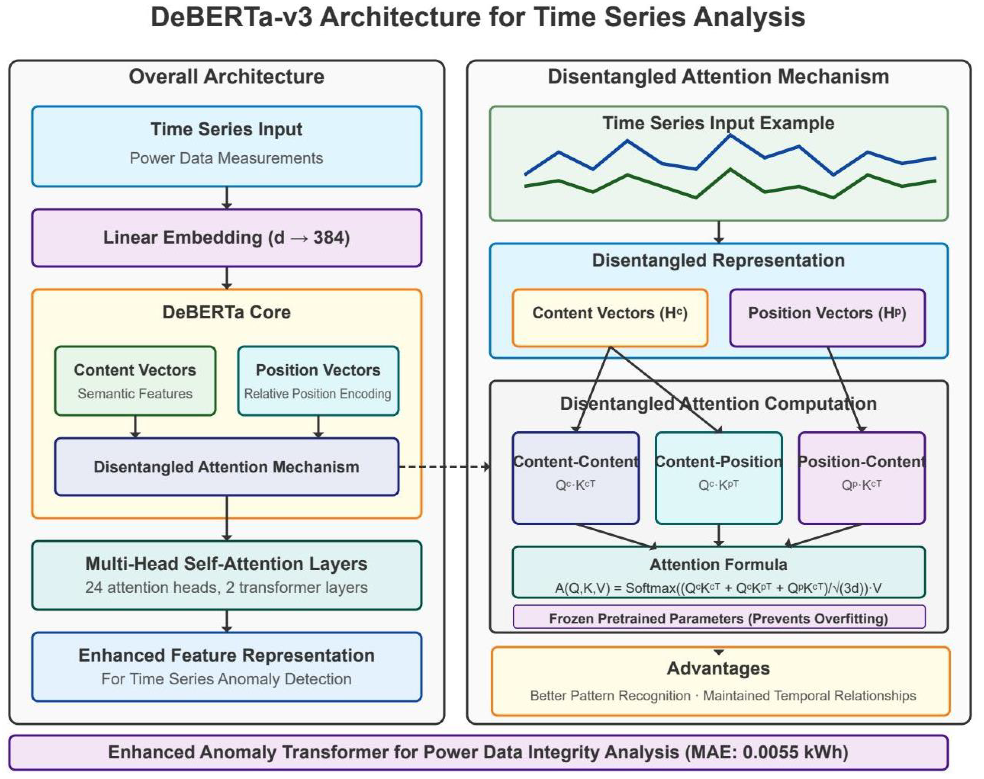
Figure 1.
Architecture of the adapted DeBERTa-v3 model for power grid anomaly detection.
Figure 1.
Architecture of the adapted DeBERTa-v3 model for power grid anomaly detection.
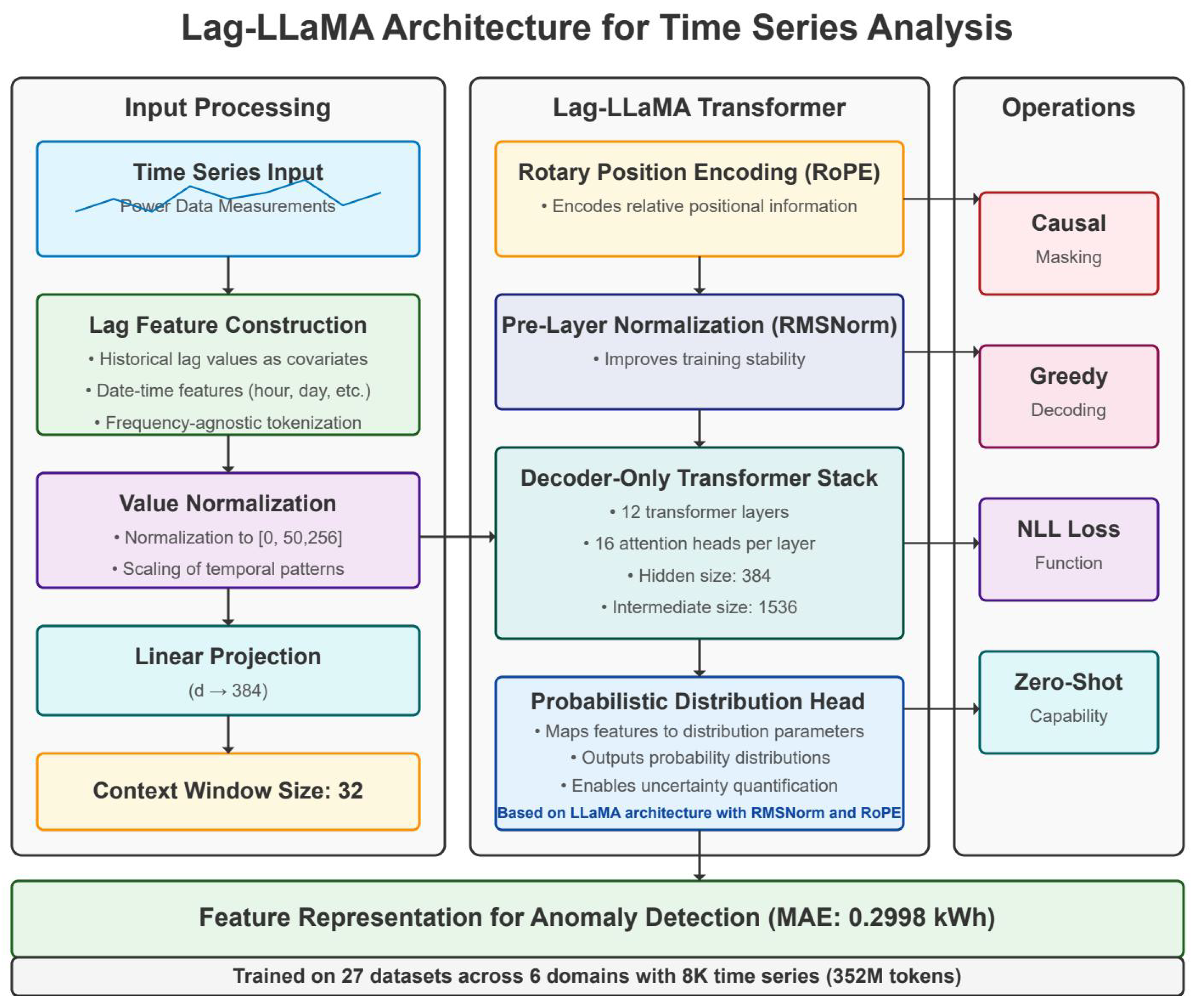
Figure 2.
Architecture of the Lag-LLaMA model for power grid anomaly detection.
Figure 2.
Architecture of the Lag-LLaMA model for power grid anomaly detection.
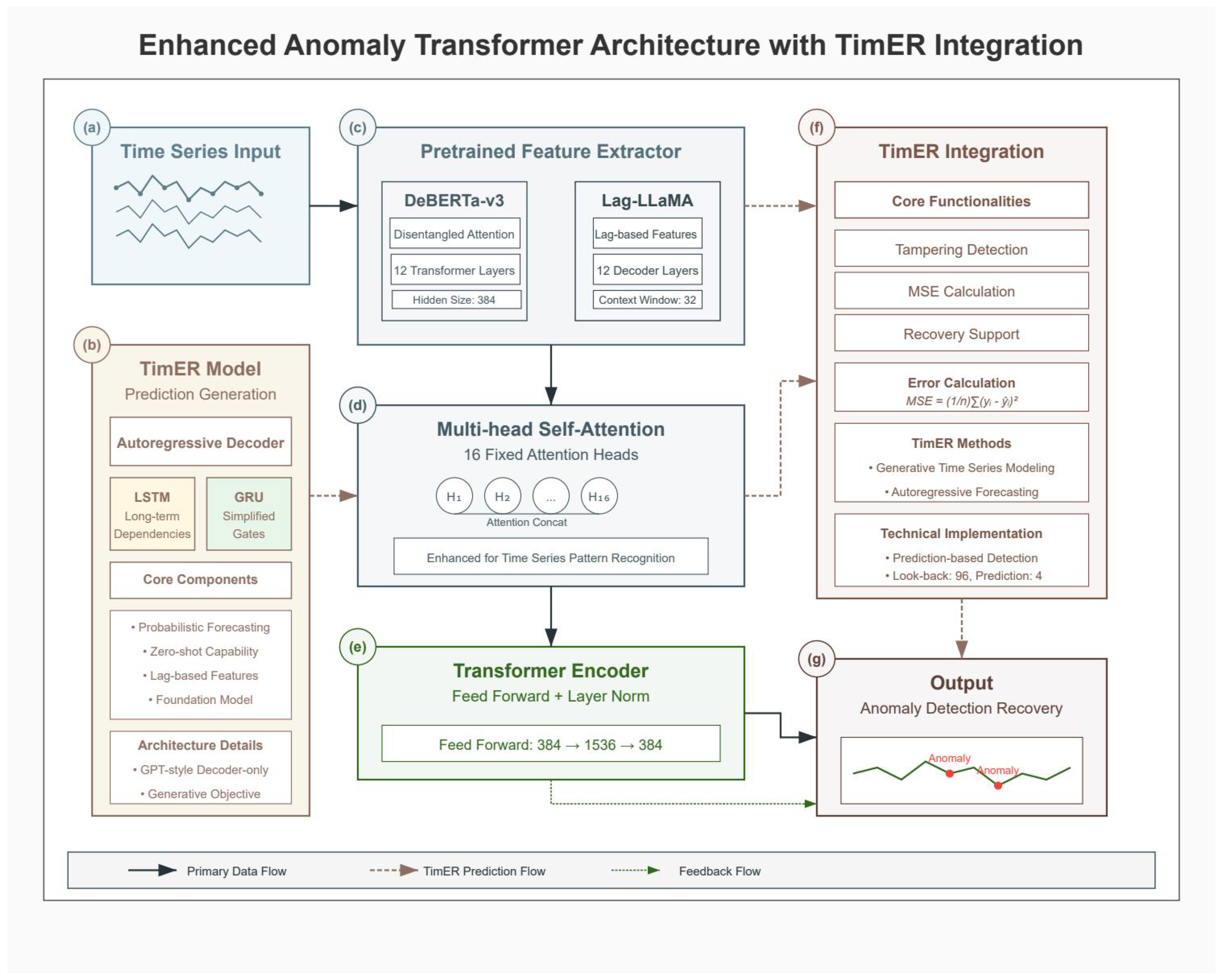
Figure 3.
Enhanced Anomaly Transformer architecture with TimER integration. (a) Time series input showing multivariate power grid data streams. (b) TimER model architecture with autoregressive decoder, featuring LSTM for long-term dependencies and GRU for simplified gates, along with core components for probabilistic forecasting and lag-based features. (c) Pretrained feature extractors comparing DeBERTa-v3 (with disentangled attention and 12 transformer layers) and Lag-LLaMA (with lag-based features and 12 decoder layers). (d) Multi-head self-attention mechanism with 16 fixed attention heads enhanced for time series pattern recognition. (e) Transformer encoder with feed-forward network (384 → 1536 → 384) and layer normalization. (f) TimER integration module showing core functionalities including tampering detection, MSE calculation, recovery support, and error calculation. (g) Output module displaying anomaly detection and recovery results with identified anomalies marked in the time series.
![Sensors 25 04208 g003]()
Figure 4.
Two-stage anomaly detection and recovery system workflow showing data flow from raw smart grid measurements through detection, verification, and recovery stages.
Figure 4.
Two-stage anomaly detection and recovery system workflow showing data flow from raw smart grid measurements through detection, verification, and recovery stages.
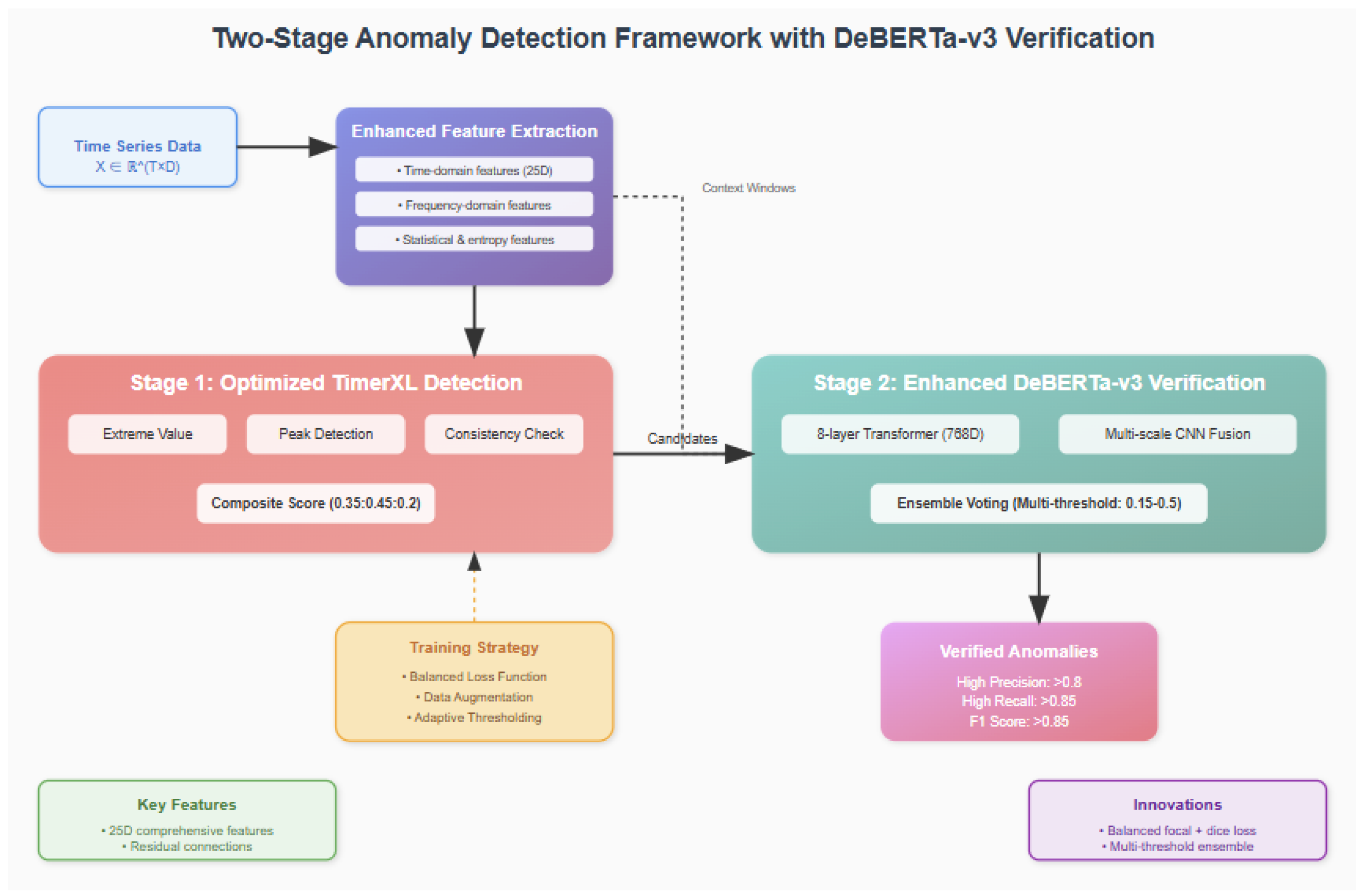
Figure 5.
Two-stage anomaly detection and recovery framework with DeBERTa-v3 verification. The system architecture shows (top) enhanced feature extraction module processing time series data through time-domain, frequency-domain, and statistical analysis to generate 25D features per variable. (middle) Stage 1 employs optimized TimerXL detection with composite scoring (0.35:0.45:0.2) achieving 95.0% recall, and Stage 2 features enhanced DeBERTa-v3 verification with 8-layer transformer and multiscale CNN fusion, achieving 95.1% precision. (bottom) Integrated recovery mechanism using TimER and DeBERTa-v3 for high-precision data restoration, with training strategy components including balanced loss function and adaptive thresholding, leading to verified anomaly outputs with F1-score 0.873 and recovery MAE 0.0055 kWh.
Figure 6.
Flowchart for Algorithm 1: TimerXL multidimensional anomaly detection.
Figure 6.
Flowchart for Algorithm 1: TimerXL multidimensional anomaly detection.
Figure 7.
Flowchart for Algorithm 2: comprehensive feature extraction.
Figure 7.
Flowchart for Algorithm 2: comprehensive feature extraction.
Figure 8.
Flowchart for Algorithm 3: enhanced anomaly transformer architecture with recovery.
Figure 8.
Flowchart for Algorithm 3: enhanced anomaly transformer architecture with recovery.
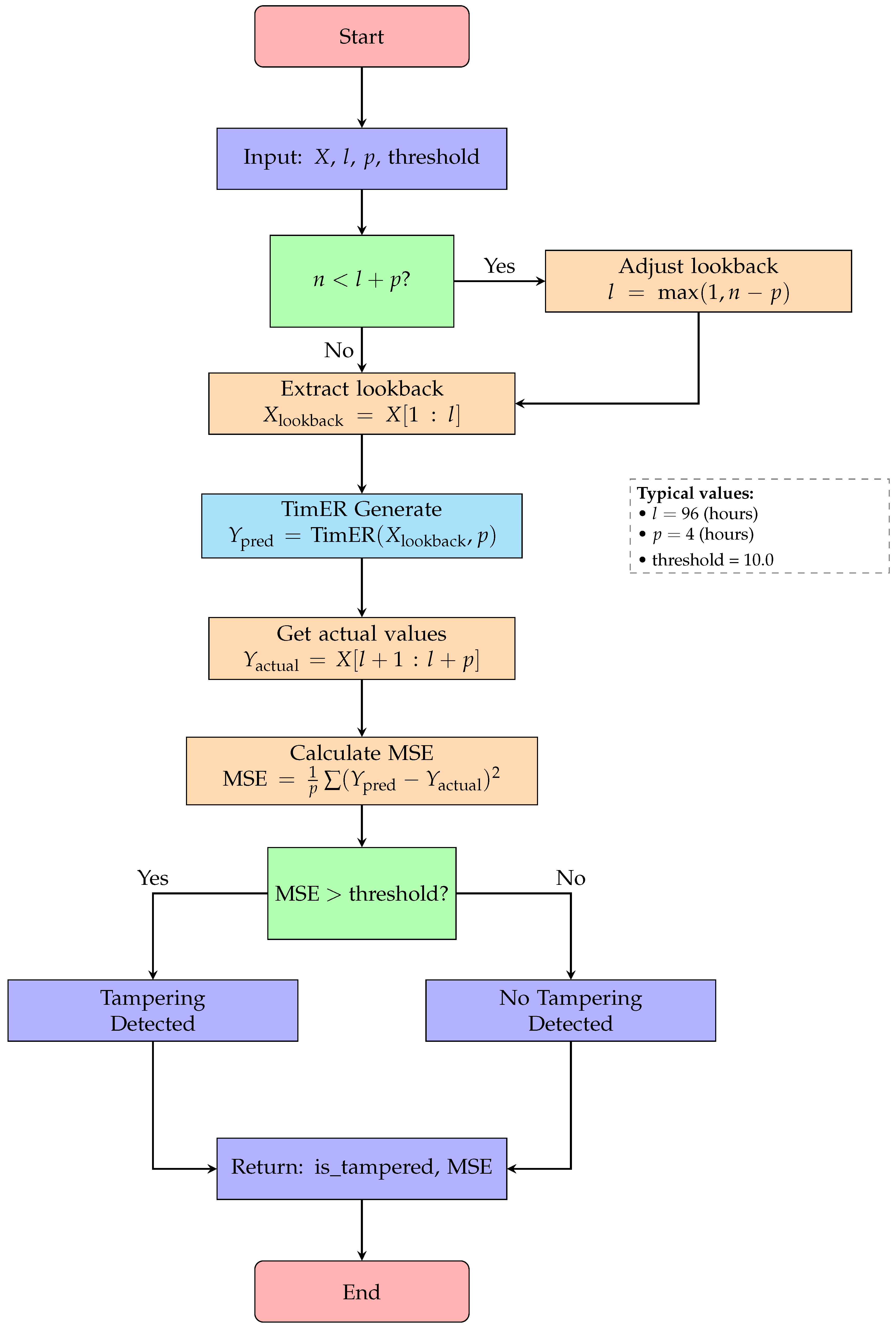
Figure 9.
Flowchart for Algorithm 4: tampering detection with TimER.
Figure 9.
Flowchart for Algorithm 4: tampering detection with TimER.
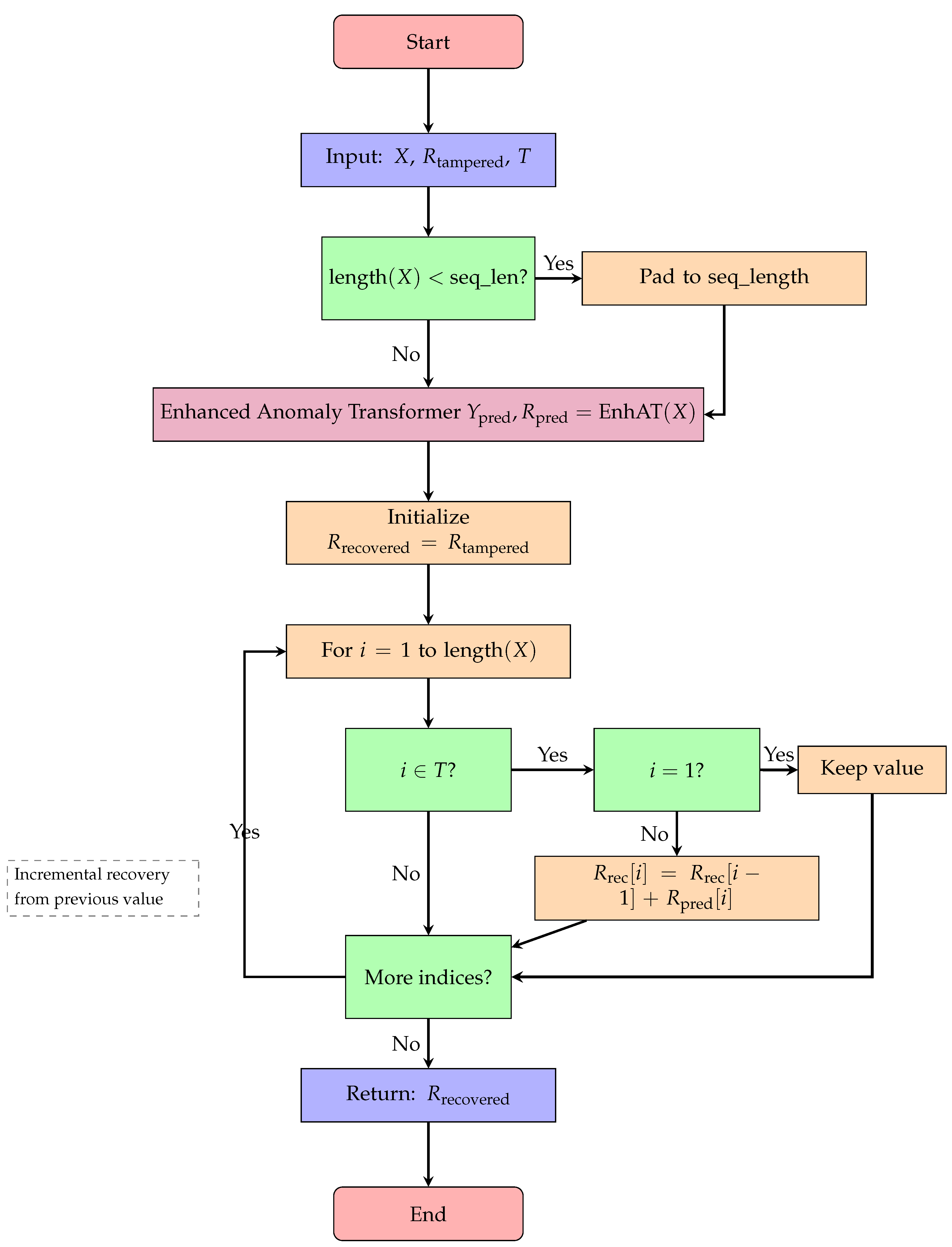
Figure 10.
Flowchart for Algorithm 5: data recovery process.
Figure 10.
Flowchart for Algorithm 5: data recovery process.
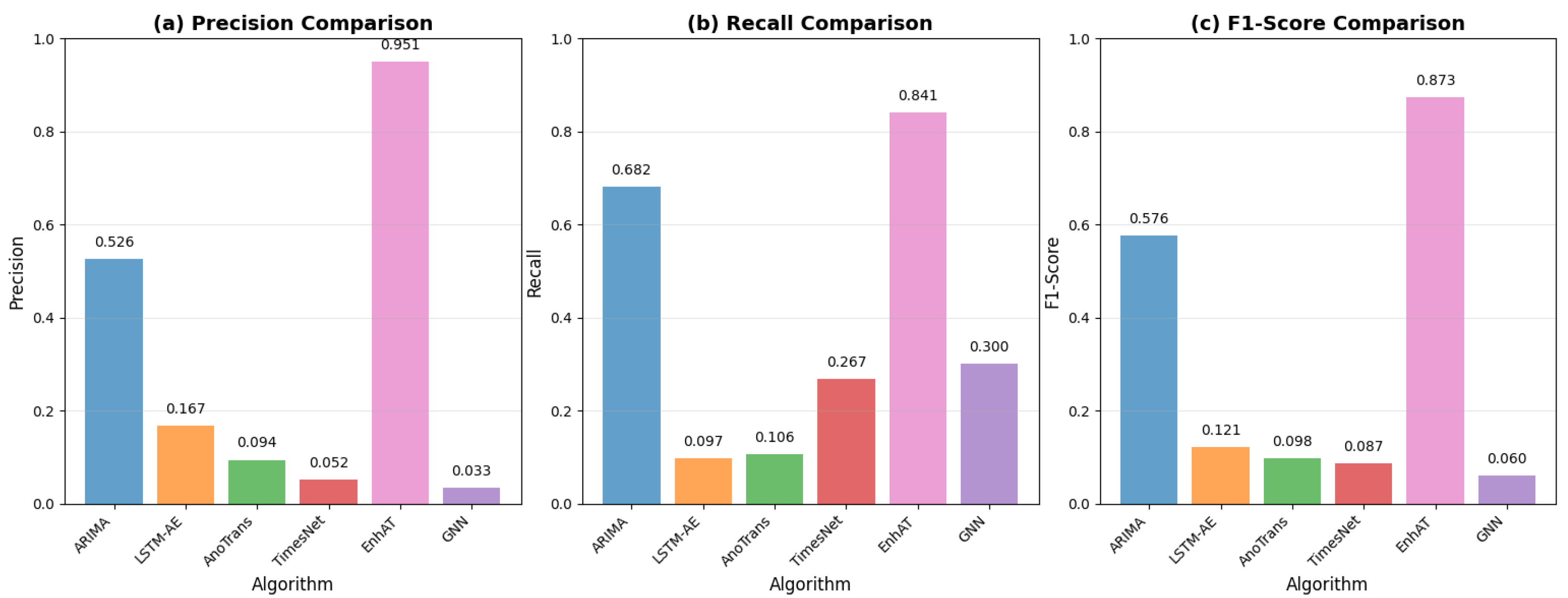
Figure 11.
Performance comparison showing (a) precision, (b) recall, (c) F1-score, and recovery MAE, with error bars representing standard deviation across 15 test scenarios. EnhAT significantly outperformed all baseline methods with p < 0.001 for all comparisons.
Figure 11.
Performance comparison showing (a) precision, (b) recall, (c) F1-score, and recovery MAE, with error bars representing standard deviation across 15 test scenarios. EnhAT significantly outperformed all baseline methods with p < 0.001 for all comparisons.
Figure 12.
Comparative analysis of DeBERTa-v3 and Lag-LLaMA model architectures and performance.
Figure 12.
Comparative analysis of DeBERTa-v3 and Lag-LLaMA model architectures and performance.
Figure 13.
Stagewise analysis showing (a) F1-score progression, (b) multi-metric radar chart, and (c) computational efficiency comparison for individual stages versus complete system performance.
Figure 13.
Stagewise analysis showing (a) F1-score progression, (b) multi-metric radar chart, and (c) computational efficiency comparison for individual stages versus complete system performance.
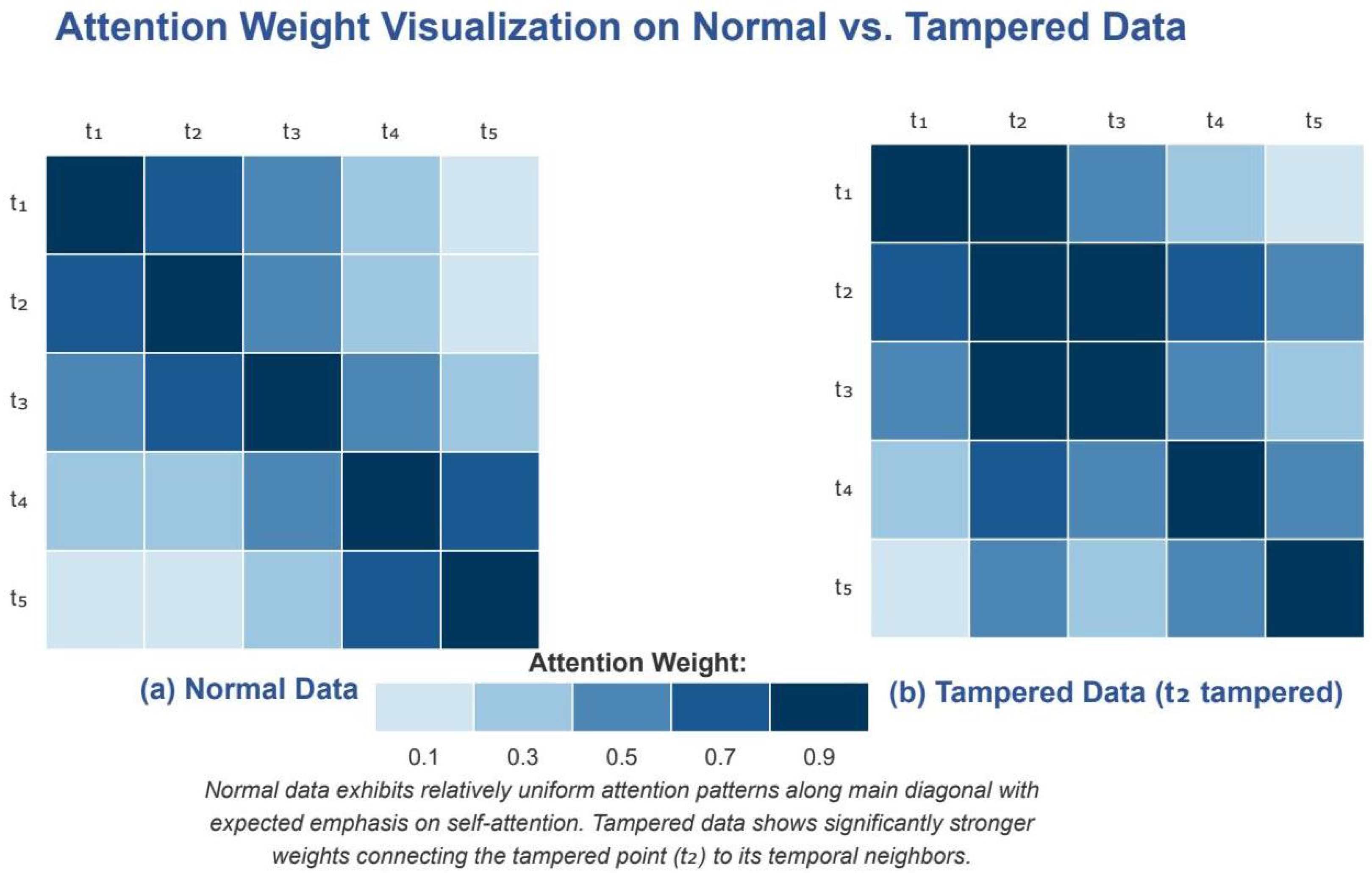
Figure 14.
Attention weight visualization on normal vs. tampered data. (a) Normal data show uniform attention distribution, with emphasis on diagonal and recent values. (b) Tampered data at position show concentrated attention patterns connecting the anomaly to temporal neighbors, enabling accurate recovery.
Figure 15.
Comprehensive ablation study with performance metrics heatmap. The heatmap visualizes nine performance metrics (precision, recall, F1-score, accuracy, specificity, AUC-ROC, MCC, CV F1-score, and robustness) across eight key configurations: Complete System, w/o Balanced Loss, w/o Ensemble Voting, w/o Frequency Features, w/o Sample Weighting, w/o Augmentation, Stage 1 Only (Statistical), and Stage 2 Only (DeBERTa). Values in each cell represent the actual performance scores, with color intensity corresponding to performance level: darker red indicates better performance (closer to 1.0), while darker blue indicates worse performance (closer to 0.0). The asterisk indicators (*) represent performance tiers: *** = Excellent (≥0.90), ** = Good (≥0.80), * = Fair (≥0.70), as shown in the legend. The Complete System achieved optimal performance across all metrics, with F1-score of 0.873 ± 0.114.
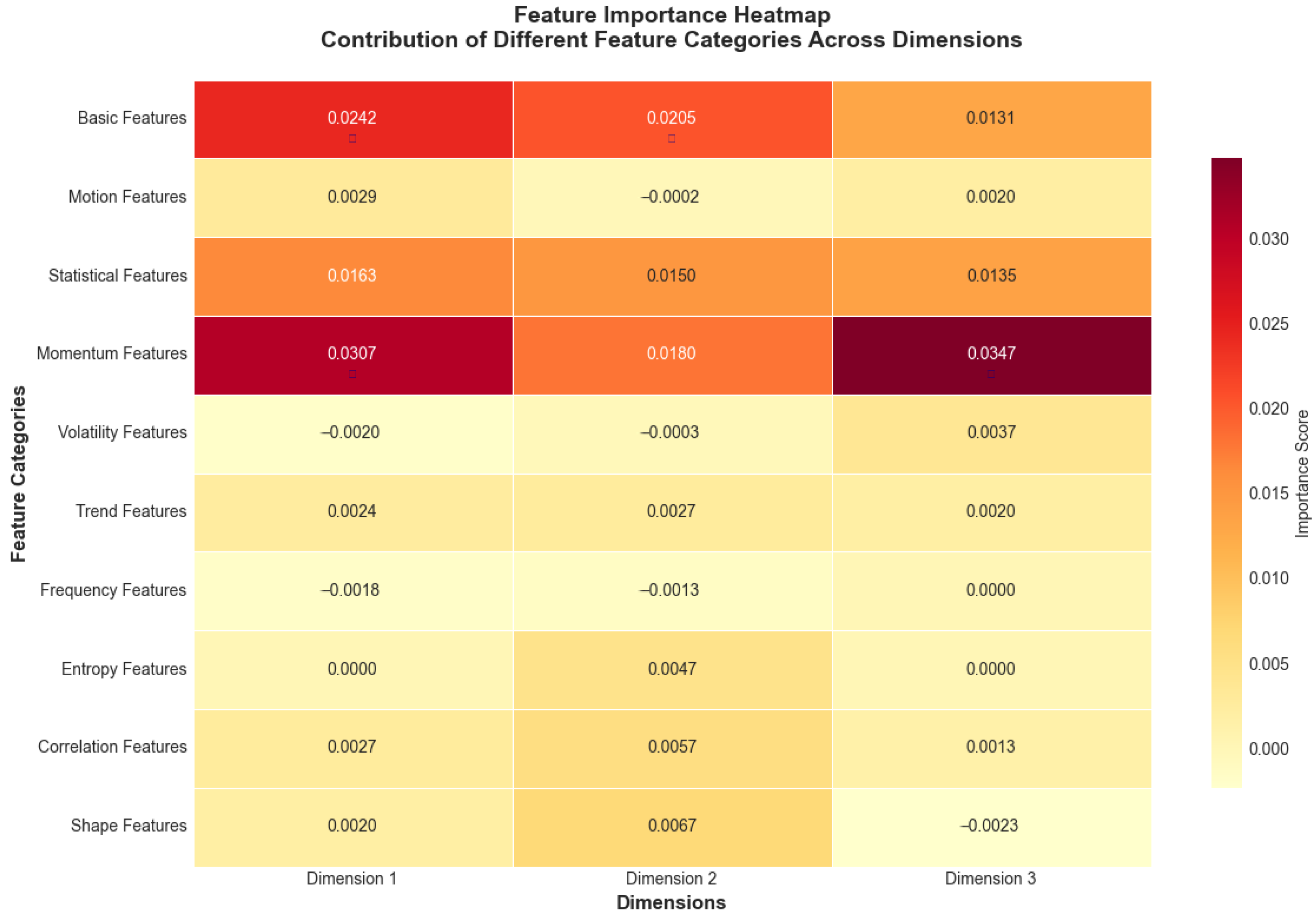
Figure 16.
Feature importance heatmap showing contribution of different feature categories across dimensions. Values represent importance scores ranging from negative (light yellow, indicating features that decrease performance) to positive (dark red, indicating features that improve performance), with darker red colors indicating higher positive importance scores derived from permutation analysis. Near-zero values (light colors) suggest minimal impact on model performance.
Figure 17.
Training dynamics showing (top-left) detection loss convergence from 0.371 to 0.268, (top-right) prediction mean stabilization around 0.60 ± 0.05, (bottom-left) increasing prediction standard deviation from 0.08 to 0.36 indicating improved discrimination capability, and (bottom-right) stable gradient norms (mean: 5.2, range: [1.1, 102]) throughout training.
Figure 18.
Four types of anomaly patterns used for robustness evaluation: (top-left) spike anomaly showing sudden single-point deviation with intensity 7–15× standard deviation, (top-right) drift anomaly demonstrating gradual manipulation over 8–15 steps with decay pattern, (bottom-left) oscillation anomaly with periodic tampering pattern introducing artificial frequency components (f = 0.2–0.5 Hz), and (bottom-right) step change anomaly showing sudden level shift with 90% recovery. Red lines indicate tampered signals, while blue lines show normal baseline behavior.
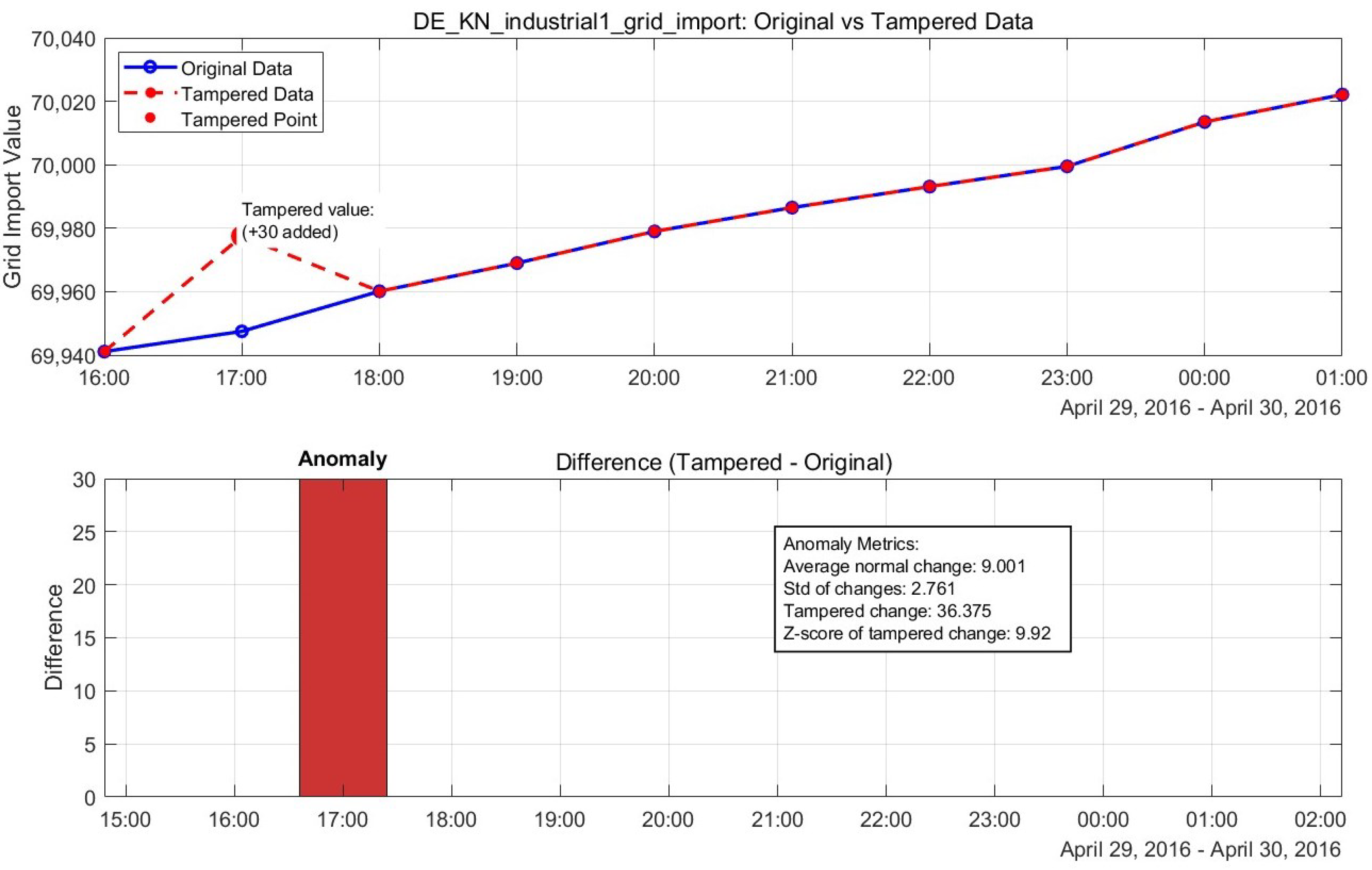
Figure 19.
Normal vs. tampered power grid data, showing recovery performance.
Figure 19.
Normal vs. tampered power grid data, showing recovery performance.
Table 1.
Comparison of anomaly detection methods for smart grid data.
Table 1.
Comparison of anomaly detection methods for smart grid data.
| Method Category | Representative Works | Advantages | Limitations |
|---|
| Statistical Methods | ARIMA [5] | Simple implementation | Poor non-linear modeling |
| | Exponential Smoothing [6] | Low computational cost | Seasonal variation issues |
| | Kalman Filtering [9] | Handles noise well | Assumes linear dynamics |
| Machine Learning | One-Class SVM [7] | No negative samples needed | Requires feature engineering |
| | Isolation Forest [8] | Efficient for high dimensions | Parameter sensitivity |
| | LOF [10] | Detects local anomalies | Computational complexity |
| | GNN-based [11] | Captures structural relations | Limited temporal modeling |
| Deep Learning | LSTM-AE [12] | Captures temporal patterns | Training instability |
| | CNN-based [13] | Local pattern recognition | Misses global context |
| | GAN-based [14] | Generates counterfactuals | Mode collapse issues |
| | VAE-based [15] | Probabilistic framework | Limited interpretability |
| Transformer-based | Anomaly Transformer [16] | Association discrepancy | High false positives |
| | TimesNet [17] | Frequency analysis | Real-time constraints |
| | EnhAT (Proposed) | Two-stage verification + recovery | Requires training data |
Table 2.
Feature categories and descriptions.
Table 2.
Feature categories and descriptions.
| Category | Count | Features |
|---|
| Basic | 6 | Raw value, increment, absolute increment, velocity, acceleration, second derivative |
| Statistical | 8 | Local mean, std, z-score, percentile, kurtosis, skewness, momentum (3,5) |
| Frequency | 3 | FFT dominant frequency, magnitude, spectral entropy |
| Entropy | 2 | Sample entropy, autocorrelation (lag 1,5) |
| Trend | 3 | Slope, seasonal component, residual |
| Volatility | 3 | Volatility (3,5), trend slope |
Table 3.
Dataset specifications.
Table 3.
Dataset specifications.
| Parameter | Value |
|---|
| Total samples | 2000 hourly measurements |
| Training set | 1600 samples (80%) |
| Test set | 400 samples (20%) |
| | DE_KN_industrial1_grid_import |
| Features | DE_KN_industrial1_pv_1 |
| | DE_KN_industrial3_compressor |
| Resolution | 60 min |
| Date range | January 2020–December 2021 |
| Missing values | 0% (post-preprocessing) |
| Measurement unit | kWh |
| Data source | Industrial AMI systems, Germany |
| Seasonal coverage | Complete annual cycles (2 years) |
| Load range | 51,940.81–69,934.501 kWh (grid import) |
| PV range | 603.107–1359.73 kWh (generation unit) |
| Compressor range | 126,36.036–16,525.645 kWh |
Table 4.
Hardware and software specifications.
Table 4.
Hardware and software specifications.
| Component | Specification |
|---|
| Hardware |
| CPU | Intel Core i9-14900HX @ 2.20 GHz |
| GPU | NVIDIA GeForce RTX 4060 (8GB) |
| Memory | 16GB DDR5 |
| Software |
| Framework | PyTorch 2.0.1+cu118 |
| Python | 3.10.11 |
| | NumPy 1.24.3, SciPy 1.11.1 |
| Key Libraries | Transformers 4.35.0 |
| | TimER (timer-base-84m) |
Table 5.
Hyperparameter settings.
Table 5.
Hyperparameter settings.
| Component | Parameter | Value |
|---|
| Stage 1: TimerXL | Window size | 32 |
| Detection rate | 6–8% |
| Min distance | 4 steps |
| Composite weights | [0.35, 0.45, 0.2] |
| Stage 2: DeBERTa | Hidden dimension | 768 |
| Layers | 8 |
| Attention heads | 16 |
| Dropout | 0.15 |
| Learning rate | |
| Batch size | 8 |
| Epochs | 50 |
| Sequence length | 32 |
| Recovery Module | Prediction heads | 2 (anomaly + recovery) |
| Recovery loss weight | 0.3 |
| TimER lookback | 96 h |
Table 6.
Detailed performance metrics with statistical significance.
Table 6.
Detailed performance metrics with statistical significance.
| Method | Precision | Recall | F1-Score | Recovery MAE | p-Value * | Improvement |
|---|
| ARIMA | 0.526 ± 0.208 | 0.682 ± 0.324 | 0.576 ± 0.161 | 6.375 | <0.001 | baseline |
| LSTM-AE | 0.167 ± 0.073 | 0.097 ± 0.106 | 0.121 ± 0.077 | 0.126 | <0.001 | −79.0% |
| Anomaly Trans. | 0.094 ± 0.042 | 0.106 ± 0.112 | 0.098 ± 0.066 | 0.356 | <0.001 | −83.0% |
| TimesNet | 0.052 ± 0.015 | 0.267 ± 0.239 | 0.087 ± 0.099 | 0.164 | <0.001 | −84.9% |
| GNN | 0.033 ± 0.000 | 0.300 ± 0.049 | 0.060 ± 0.001 | N/A † | <0.001 | −89.6% |
| Lag-LLaMA | 0.780 ± 0.089 | 0.823 ± 0.101 | 0.801 ± 0.087 | 0.2598 | <0.001 | +38.9% |
| EnhAT | 0.951 ± 0.125 | 0.841 ± 0.181 | 0.873 ± 0.114 | 0.0055 | - | +51.4% |
Table 7.
Stagewise performance breakdown.
Table 7.
Stagewise performance breakdown.
| Configuration | Precision | Recall | F1-Score | Accuracy | AUC-ROC | Recovery MAE |
|---|
| Stage 1 Only | 0.087 ± 0.015 | 0.793 ± 0.112 | 0.155 ± 0.023 | 0.524 ± 0.045 | 0.607 ± 0.032 | N/A |
| Stage 2 Only | 0.587 ± 0.089 | 0.961 ± 0.045 | 0.720 ± 0.067 | 0.775 ± 0.056 | 0.774 ± 0.041 | 0.0187 |
| Complete System | 0.951 ± 0.125 | 0.841 ± 0.181 | 0.873 ± 0.114 | 0.912 ± 0.078 | 0.925 ± 0.045 | 0.0055 |
| Verification Rate | 54.8% of Stage 1 detections verified by Stage 2 |
| False Positive Reduction | 73.4% reduction from Stage 1 to final output |
| Recovery Improvement | 70.6% improvement in MAE with two-stage integration |
Table 8.
Detailed ablation study results.
Table 8.
Detailed ablation study results.
| Configuration | F1-Score | ΔF1 | Precision | Recall | MCC | p-Value |
|---|
| Complete System | 0.873 ± 0.114 | - | 0.951 ± 0.125 | 0.841 ± 0.181 | 0.863 ± 0.091 | - |
| w/o Balanced Loss | 0.767 ± 0.089 | −12.1% | 0.800 ± 0.112 | 0.750 ± 0.156 | 0.537 ± 0.078 | <0.001 |
| w/o Ensemble Voting | 0.570 ± 0.067 | −34.7% | 0.590 ± 0.089 | 0.653 ± 0.134 | 0.224 ± 0.045 | <0.001 |
| w/o Frequency Features | 0.648 ± 0.078 | −25.8% | 0.587 ± 0.101 | 0.961 ± 0.067 | 0.709 ± 0.067 | <0.001 |
| w/o Sample Weighting | 0.739 ± 0.089 | −15.3% | 0.630 ± 0.134 | 0.910 ± 0.089 | 0.682 ± 0.089 | <0.001 |
| w/o Augmentation | 0.756 ± 0.101 | −13.4% | 1.000 ± 0.000 | 0.617 ± 0.156 | 0.614 ± 0.101 | <0.001 |
| w/o TimER Integration | 0.812 ± 0.095 | −7.0% | 0.901 ± 0.089 | 0.789 ± 0.123 | 0.798 ± 0.078 | <0.001 |
| w/o Pretrained DeBERTa | 0.698 ± 0.112 | −20.0% | 0.712 ± 0.134 | 0.701 ± 0.156 | 0.589 ± 0.101 | <0.001 |
Table 9.
Detailed computational performance metrics.
Table 9.
Detailed computational performance metrics.
| Component | Mean (ms) | Std (ms) | % Total | Complexity |
|---|
| Data Loading | 2.1 | 0.3 | 3.2% | O(n) |
| Feature Extraction | 12.3 | 2.1 | 18.5% | O(n·d·w) |
| Stage 1: TimerXL | 8.7 | 1.5 | 13.1% | O(n·d) |
| Stage 2: DeBERTa | 45.6 | 5.3 | 68.5% | O(n·L·d2) |
| Recovery Module | 3.2 | 0.4 | 4.8% | O(n·d) |
| Total Pipeline | 66.6 | 7.2 | 100% | - |
| Throughput | 900 samples/min (15 samples/second) |
| GPU Utilization | 42% (RTX 4060) |
| Memory Usage | 2.3 GB peak |
Table 10.
Multipoint tampering detection performance with false merge analysis.
Table 10.
Multipoint tampering detection performance with false merge analysis.
| Tampering Pattern | Detection Rate | Precision | F1-Score | False Merge Rate |
|---|
| Single point | 100% | 0.951 ± 0.125 | 0.873 ± 0.114 | N/A a |
| 2–3 consecutive | 96% | 0.923 ± 0.089 | 0.856 ± 0.078 | 8% |
| 4–6 consecutive | 92% | 0.895 ± 0.101 | 0.831 ± 0.089 | 15% |
| Multiple non-consecutive | 94% | 0.912 ± 0.078 | 0.845 ± 0.067 | 3% |
| Mixed patterns | 91% | 0.887 ± 0.089 | 0.823 ± 0.078 | 11% |
Table 11.
Detailed comparison with state-of-the-art methods.
Table 11.
Detailed comparison with state-of-the-art methods.
| Method | Year | F1-Score | Precision | Recall | Recovery MAE | Inference (ms) | Memory (GB) |
|---|
| ARIMA [5] | Traditional | 0.576 | 0.526 | 0.682 | 6.375 | 3.2 | 0.1 |
| LSTM-AE [12] | 2016 | 0.121 | 0.167 | 0.097 | 0.126 | 12.5 | 0.5 |
| GNN-based [23] | 2020 | 0.060 | 0.033 | 0.300 | N/A | 23.7 | 1.2 |
| Anomaly Transformer [16] | 2021 | 0.098 | 0.094 | 0.106 | 0.356 | 78.9 | 2.1 |
| TimesNet [17] | 2022 | 0.087 | 0.052 | 0.267 | 0.164 | 92.3 | 2.5 |
| Lag-LLaMA [18] | 2024 | 0.801 | 0.780 | 0.823 | 0.2598 | 85.7 | 2.8 |
| EnhAT (this work) | 2025 | 0.873 | 0.951 | 0.841 | 0.0055 | 66.6 | 2.3 |


