
Ensembling a Learned Volterra Polynomial with a Neural Network for Joint Nonlinear Distortions and Mismatch Errors Calibration of Time-Interleaved Pipelined ADCs

Abstract
1. Introduction
2. Comprehensive Analysis of Nonlinear Distortions and Mismatch Errors in TI-Pipelined ADCs
2.1. Nonlinear Distortions
2.2. Mismatch Errors
2.2.1. Offset Mismatch and Gain Mismatch
2.2.2. Timing Skew Mismatch
2.3. Comprehensive Analysis
3. Learned Volterra–Neural Network Ensemble Model
3.1. Overall Architecture
3.2. Learned Volterra Front-End: Static Baseline Distortion Forward Mapping
3.3. Neural Network Back-End: Dynamic Nonlinear Distortion and Mismatch Error Inverse Mapping
4. Dataset Construction and Training of the Ensemble Model
5. Results and Discussion
5.1. Simulation Results
5.2. Measurement Results
5.3. Ablation Analysis of Our Ensemble Model
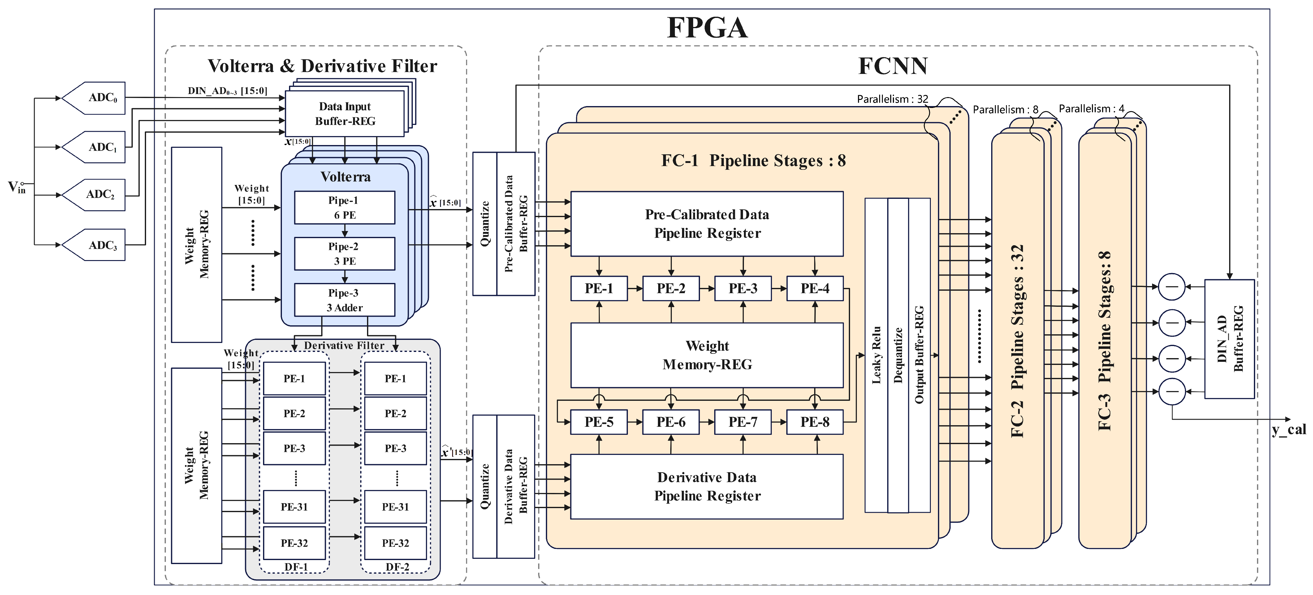
5.4. Hardware Implementation
6. Conclusions
Author Contributions
Funding
Institutional Review Board Statement
Informed Consent Statement
Data Availability Statement
Conflicts of Interest
References
- Lyu, Y.; Hu, Y. A Matching Strategy Based on Full-Permutation Bisection for Data Converters. IEEE Trans. Circuits Syst. I Regul. Pap. 2023, 70, 2711–2721. [Google Scholar] [CrossRef]
- Gagliardi, F.; Scintu, D.; Piotto, M.; Bruschi, P.; Dei, M. Static-Linearity Enhancement Techniques for Digital-to-Analog Converters Exploiting Optimal Arrangements of Unit Elements. IEEE Trans. Very Large Scale Integr. Syst. 2024, 32, 2243–2256. [Google Scholar] [CrossRef]
- Wu, K.C.; Wu, M.S.; Hong, H.C. Multiple correlation estimation based digital background calibration scheme for pipelined ADCs. In Proceedings of the 2019 IEEE International Symposium on Circuits and Systems (ISCAS), Sapporo, Japan, 26–29 May 2019; pp. 1–5. [Google Scholar]
- Liu, X.; Xu, H.; Johansson, H.; Wang, Y.; Li, N. Correlation-based calibration for nonlinearity mismatches in dual-channel tiadcs. IEEE Trans. Circuits Syst. II Express Briefs 2019, 67, 585–589. [Google Scholar]
- Niu, H.; Yuan, J. A spectral-correlation-based blind calibration method for time-interleaved ADCs. IEEE Trans. Circuits Syst. I Regul. Pap. 2020, 67, 5007–5017. [Google Scholar] [CrossRef]
- Ni, M.; Wang, X.; Li, F.; Rhee, W.; Wang, Z. A 13-bit 2-GS/s time-interleaved ADC with improved correlation-based timing skew calibration strategy. IEEE Trans. Circuits Syst. I Regul. Pap. 2021, 69, 481–494. [Google Scholar] [CrossRef]
- Xiang, Y.; Zhou, D.; Song, M.; Zhai, D.; Lan, J.; Ren, J.; Ye, F. A Comprehensive Digital Calibration for Pipelined ADCs Using Cascaded Nonlinearity Correction. IEEE Trans. Very Large Scale Integr. Syst. 2025, 33, 1192–1196. [Google Scholar] [CrossRef]
- Shi, L.; Zhao, W.; Wu, J.; Chen, C. Digital background calibration techniques for pipelined ADC based on comparator dithering. IEEE Trans. Circuits Syst. II Express Briefs 2012, 59, 239–243. [Google Scholar] [CrossRef]
- Moosazadeh, T.; Yavari, M. A calibration technique for pipelined ADCs using self-measurement and histogram-based test methods. IEEE Trans. Circuits Syst. II Express Briefs 2015, 62, 826–830. [Google Scholar] [CrossRef]
- Jiani, M.; Shoaei, O. Fast background calibration of linear and non-linear errors in pipeline analog-to-digital converters. IEEE Trans. Circuits Syst. II Express Briefs 2021, 69, 884–888. [Google Scholar] [CrossRef]
- Cao, W.; Yu, C.; Zhu, A. Digital post-correction of analog-to-digital converters with real-time FPGA implementation. In Proceedings of the 2015 26th Irish Signals and Systems Conference (ISSC), Carlow, Ireland, 24–25 June 2015; pp. 1–4. [Google Scholar]
- Qiu, Y.; Zhou, J.; Liu, Y.; Huangfu, Y. A Novel Calibration Method of Gain and Time-skew Mismatches for Time-interleaved ADCs Based on Neural Network. In Proceedings of the 2019 IEEE MTT-S International Wireless Symposium (IWS), Guangzhou, China, 19–22 May 2019; pp. 1–3. [Google Scholar]
- Chen, M.; Wu, Y.; Lan, J.; Ye, F.; Chen, C.; Ren, J. A calibration scheme for nonlinearity of the SAR-pipelined ADCs based on a shared neural network. In Proceedings of the IEEE Asia Pacific Conference on Circuits and Systems (APCCAS), Ha Long, Vietnam, 8–10 December 2020; pp. 205–208. [Google Scholar]
- Chen, M.; Zhao, Y.; Xu, N.; Ye, F.; Ren, J. A partially binarized and fixed neural network based calibrator for SAR-pipelined ADCs achieving 95.0-dB SFDR. In Proceedings of the 2021 IEEE International Symposium on Circuits and Systems (ISCAS), Daegu, Republic of Korea, 22–28 May 2021; pp. 1–4. [Google Scholar]
- Zhai, D.; Jiang, W.; Jia, X.; Lan, J.; Guo, M.; Sin, S.W.; Ye, F.; Liu, Q.; Ren, J.; Chen, C. High-speed and time-interleaved adcs using additive-neural-network-based calibration for nonlinear amplitude and phase distortion. IEEE Trans. Circuits Syst. I Regul. Pap. 2022, 69, 4944–4957. [Google Scholar] [CrossRef]
- Peng, X.; Ye, X.; Liu, H.; Lu, Z.; Xiao, Y.; Peng, Y.; Tang, H. A neural network based calibration technique for TI-ADCs with derivative information. In Proceedings of the 2023 IEEE International Symposium on Circuits and Systems (ISCAS), Monterey, CA, USA, 21–25 May 2023; pp. 1–5. [Google Scholar]
- Peng, Y.; Xiao, Y.; Chen, L.; Tang, H.; Peng, X. A Novel Calibration Algorithm for ADCs Based on Inverse Mapping by Neural Network. IEEE Trans. Circuits Syst. II Express Briefs 2024, 71, 3283–3287. [Google Scholar] [CrossRef]
- Ware, E.; Correll, J.; Lee, S.; Flynn, M. 6GS/s 8-channel CIC SAR TI-ADC with neural network calibration. In Proceedings of the ESSCIRC 2022—IEEE 48th European Solid State Circuits Conference (ESSCIRC), Milan, Italy, 19–22 September 2022; pp. 325–328. [Google Scholar]
- Lu, Z.; Zhang, B.; Peng, X.; Liu, H.; Ye, X.; Li, Y.; Peng, Y.; Xiao, Y.; Zhang, W.; Tang, H. A New Artificial Neural Network-Based Calibration Mechanism for ADCs: A Time-Interleaved ADC Case Study. IEEE Trans. Very Large Scale Integr. Syst. 2024, 32, 1184–1194. [Google Scholar] [CrossRef]
- Ali, A.M.; Dinc, H.; Bhoraskar, P.; Bardsley, S.; Dillon, C.; McShea, M.; Periathambi, J.P.; Puckett, S. A 12-b 18-GS/s RF sampling ADC with an integrated wideband track-and-hold amplifier and background calibration. IEEE J. Solid-State Circuits 2020, 55, 3210–3224. [Google Scholar] [CrossRef]
- Ali, A.M.; Dinc, H.; Bhoraskar, P.; Dillon, C.; Puckett, S.; Gray, B.; Speir, C.; Lanford, J.; Brunsilius, J.; Derounian, P.R.; et al. A 14 bit 1 GS/s RF sampling pipelined ADC with background calibration. IEEE J. Solid-State Circuits 2014, 49, 2857–2867. [Google Scholar] [CrossRef]
- Miki, T.; Morie, T.; Ozeki, T.; Dosho, S. An 11-b 300-MS/s double-sampling pipelined ADC with on-chip digital calibration for memory effects. IEEE J. Solid-State Circuits 2012, 47, 2773–2782. [Google Scholar] [CrossRef]
- Nikaeen, P.; Murmann, B. Digital compensation of dynamic acquisition errors at the front-end of high-performance A/D converters. IEEE J. Sel. Top. Signal Process. 2009, 3, 499–508. [Google Scholar] [CrossRef]
- Li, D.; Feng, T.; Ding, J.; Shen, Y.; Liu, S.; Zhu, Z. A Wideband Input Buffer Based on Cascade Complementary Source Follower. IEEE Trans. Very Large Scale Integr. Syst. 2024, 32, 962–966. [Google Scholar] [CrossRef]
- Ali, A.M.; Dinc, H.; Bhoraskar, P.; Puckett, S.; Morgan, A.; Zhu, N.; Yu, Q.; Dillon, C.; Gray, B.; Lanford, J.; et al. A 14-bit 2.5 GS/s and 5GS/s RF sampling ADC with background calibration and dither. In Proceedings of the 2016 IEEE Symposium on VLSI Circuits (VLSI-Circuits), Honolulu, HI, USA, 15–17 June 2016; pp. 1–2. [Google Scholar]
- Yuan, J.; Fung, S.W.; Chan, K.Y.; Xu, R. An interpolation-based calibration architecture for pipeline ADC with nonlinear error. IEEE Trans. Instrum. Meas. 2011, 61, 17–25. [Google Scholar] [CrossRef]
- Chen, J.; Kao, S.h.; He, H.; Zhuo, W.; Wen, S.; Lee, C.H.; Chan, S.H.G. Run, don’t walk: Chasing higher FLOPS for faster neural networks. In Proceedings of the 2023 IEEE/CVF Conference on Computer Vision and Pattern Recognition, Vancouver, BC, Canada, 17–24 June 2023; pp. 12021–12031. [Google Scholar]
- Kim, H.; Khan, M.U.K.; Kyung, C.M. Efficient neural network compression. In Proceedings of the 2019 IEEE/CVF Conference on Computer Vision and Pattern Recognition, Long Beach, CA, USA, 15–20 June 2019; pp. 12569–12577. [Google Scholar]
- Leung, F.H.F.; Lam, H.K.; Ling, S.H.; Tam, P.K.S. Tuning of the structure and parameters of a neural network using an improved genetic algorithm. IEEE Trans. Neural Netw. 2003, 14, 79–88. [Google Scholar] [CrossRef]
- Liu, S.; Lyu, N.; Cui, J.; Zou, Y. Improved blind timing skew estimation based on spectrum sparsity and ApFFT in time-interleaved ADCs. IEEE Trans. Instrum. Meas. 2018, 68, 73–86. [Google Scholar] [CrossRef]
- Xu, W.; Yao, B.; Cheng, Q.; Du, Z.; Qiu, L. A Reference Assisted Background Calibration Technique With Constant Input Impedance for Time-Interleaved ADCs. IEEE Trans. Circuits Syst. II Express Briefs 2024, 71, 4437–4441. [Google Scholar] [CrossRef]
- Esser, S.K.; McKinstry, J.L.; Bablani, D.; Appuswamy, R.; Modha, D.S. Learned step size quantization. In Proceedings of the 2020 8th International Conference on Learning Representations (ICLR), Addis Ababa, Ethiopia, 26 April–1 May 2020. [Google Scholar]


| Memory Depth | SFDR (First Order) | SFDR (Second Order) | SFDR (Third Order) | SFDR (Fourth Order) | SFDR (Fifth Order) |
|---|---|---|---|---|---|
| One | 61.85 dB | 64.37 dB | 67.37 dB | 70.38 dB | 70.11 dB |
| Two | 61.89 dB | 65.91 dB | 70.46 dB | 70.83 dB | 70.65 dB |
| Three | 61.88 dB | 64.78 dB | 69.48 dB | 70.39 dB | 70.76 dB |
| Four | 61.91 dB | 65.43 dB | 69.63 dB | 69.99 dB | 70.43 dB |
| [7] | [17] | [19] | [15] | [31] | This Work | ||
|---|---|---|---|---|---|---|---|
| ADC Architecture | Pipelined | TI-pipelined | TI-pipelined | TI-SAR | TI-SAR | TI-pipelined | TI-pipelined |
| Resolution (bit) | 12 | 12 | 12 | 10 | 12 | 12 | 16 |
| Sampling Rate (SPS) | 800 M | 600 M | 5400 M | 5000 M | 3000 M | 3000 M | 1000 M |
| Channel | 1 | 4 | 4 | 16 | 3 | 4 | 4 |
| Calibration errors | Nonlinearity | Nonlinearity and Mismatch 1 | Nonlinearity and Mismatch | Dynamic and Static Errors | , , 2 | Nonlinearity and Mismatch | Nonlinearity and Mismatch |
| Normalized Frequency | N/A | N/A | [0 0.5] | N/A | N/A | [0 0.5] | [0 0.5] |
| Calibrator Type | DFT-LMS | FCNN-based | CNN-based | FCNN-based | REF-based | FCNN-based | FCNN-based |
| SFDR (dB) | 72.1 | 71.23 | 78.25 | 72.50 | 70.0 | 79.70 | 80.90 |
| SNDR (dB) | 54.9 | 59.19 | 53.98 | 48.20 | 63.5 | 55.63 | 62.43 |
| Parameters | - | 13.19k | 51.4k | 24.61k | - | 4.4k | 4.4k |
| FLOPs | - | 106.95M | 103.55M | 11.53M | - | 8.57M | 8.57M |
| ADC Architecture | Method | SNDR (Before) | SNDR (After) | SFDR (Before) | SFDR (After) |
|---|---|---|---|---|---|
| TI-pipelined ADC1 | V-model 1 | 35.35 dB | 37.29 dB | 35.47 dB | 35.50 dB |
| TI-pipelined ADC1 | E-model 2 | 37.29 dB | 55.63 dB | 35.50 dB | 79.70 dB |
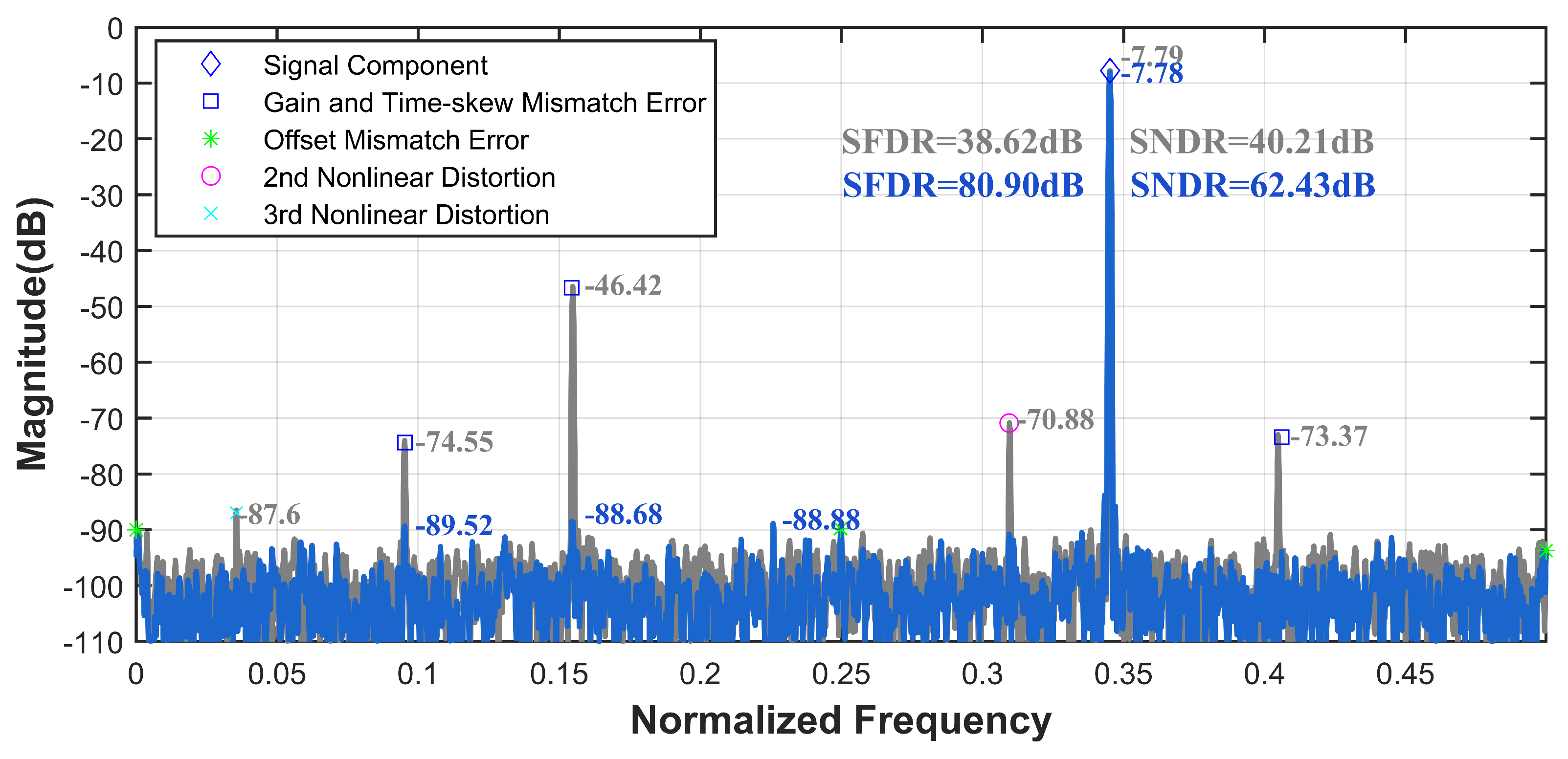
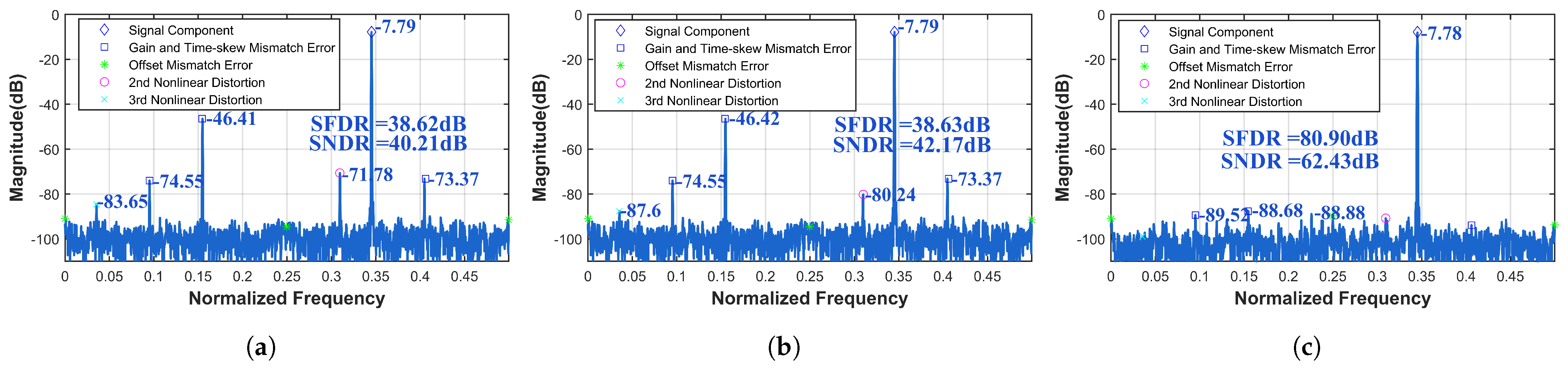
| TI-pipelined ADC2 | V-model | 40.21 dB | 42.17 dB | 38.62 dB | 38.63 dB |
| TI-pipelined ADC2 | E-model | 42.17 dB | 62.43 dB | 38.63 dB | 80.90 dB |
| Resource | Utilization | Available | Utilization % |
|---|---|---|---|
| LUT | 3480 | 341,280 | 1.02 |
| LUTRAM | 738 | 184,320 | 0.40 |
| FF | 28,800 | 682,560 | 4.22 |
| DSP | 328 | 3528 | 9.30 |
Disclaimer/Publisher’s Note: The statements, opinions and data contained in all publications are solely those of the individual author(s) and contributor(s) and not of MDPI and/or the editor(s). MDPI and/or the editor(s) disclaim responsibility for any injury to people or property resulting from any ideas, methods, instructions or products referred to in the content. |
© 2025 by the authors. Licensee MDPI, Basel, Switzerland. This article is an open access article distributed under the terms and conditions of the Creative Commons Attribution (CC BY) license (https://creativecommons.org/licenses/by/4.0/).
Share and Cite
Liu, Y.; Hao, M.; Xu, H.; Gao, X.; Zheng, H. Ensembling a Learned Volterra Polynomial with a Neural Network for Joint Nonlinear Distortions and Mismatch Errors Calibration of Time-Interleaved Pipelined ADCs. Sensors 2025, 25, 4059. https://doi.org/10.3390/s25134059
Liu Y, Hao M, Xu H, Gao X, Zheng H. Ensembling a Learned Volterra Polynomial with a Neural Network for Joint Nonlinear Distortions and Mismatch Errors Calibration of Time-Interleaved Pipelined ADCs. Sensors. 2025; 25(13):4059. https://doi.org/10.3390/s25134059
Chicago/Turabian StyleLiu, Yan, Mingyu Hao, Hui Xu, Xiang Gao, and Haiyong Zheng. 2025. "Ensembling a Learned Volterra Polynomial with a Neural Network for Joint Nonlinear Distortions and Mismatch Errors Calibration of Time-Interleaved Pipelined ADCs" Sensors 25, no. 13: 4059. https://doi.org/10.3390/s25134059
APA StyleLiu, Y., Hao, M., Xu, H., Gao, X., & Zheng, H. (2025). Ensembling a Learned Volterra Polynomial with a Neural Network for Joint Nonlinear Distortions and Mismatch Errors Calibration of Time-Interleaved Pipelined ADCs. Sensors, 25(13), 4059. https://doi.org/10.3390/s25134059