
Distributed Multi-Agent Deep Reinforcement Learning-Based Transmit Power Control in Cellular Networks


Abstract
1. Introduction
2. Related Works
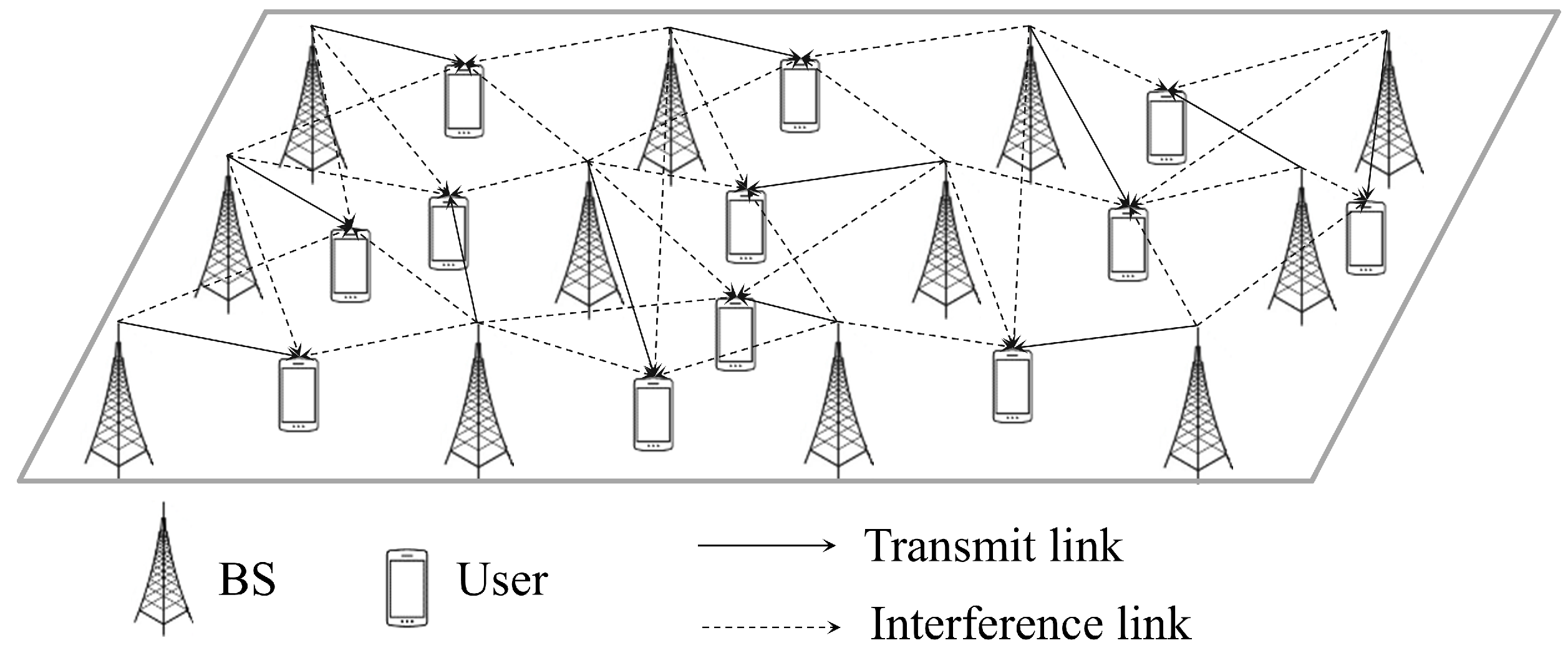
3. System Model
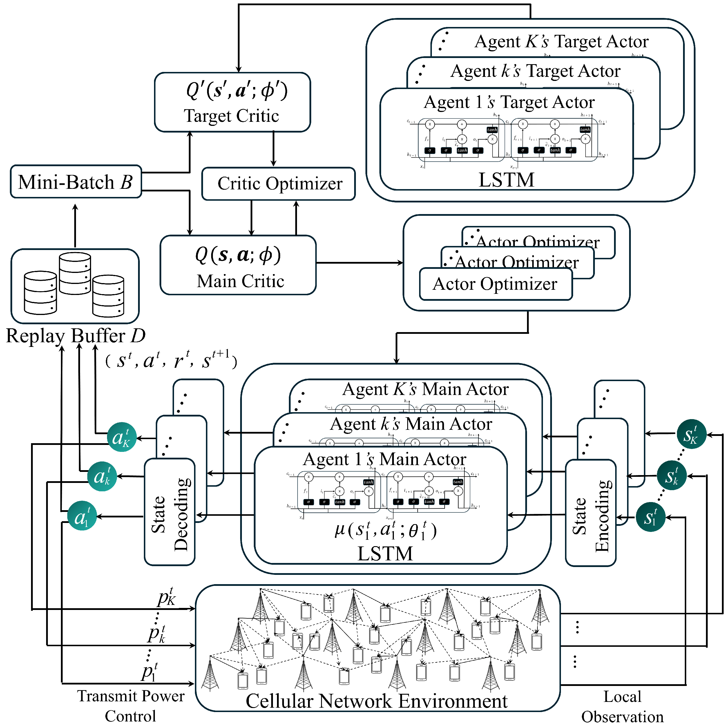
4. Proposed LSTM-Based MAAC Network for Transmit Power Control
4.1. Typical MADRL Network
4.2. Proposed MAAC Network
| Algorithm 1 The training of the proposed network with K agents. |
|
5. Simulation Results
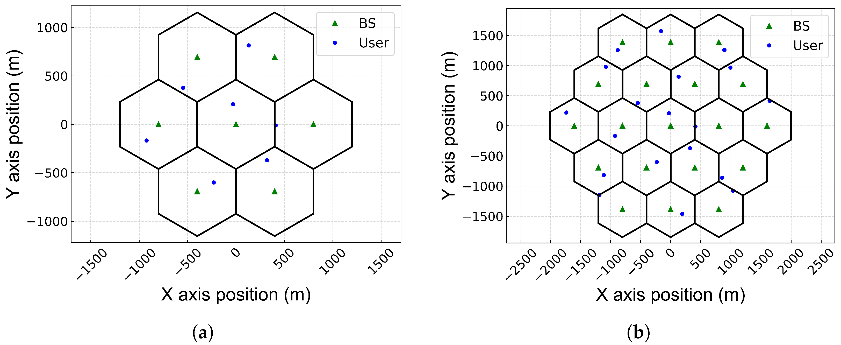
5.1. Simulation Environment
5.2. Signaling Overhead Due to Information Exchanges Between Agents
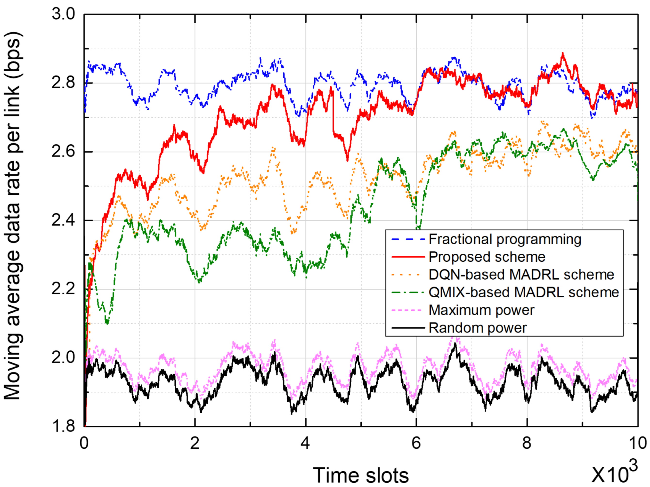
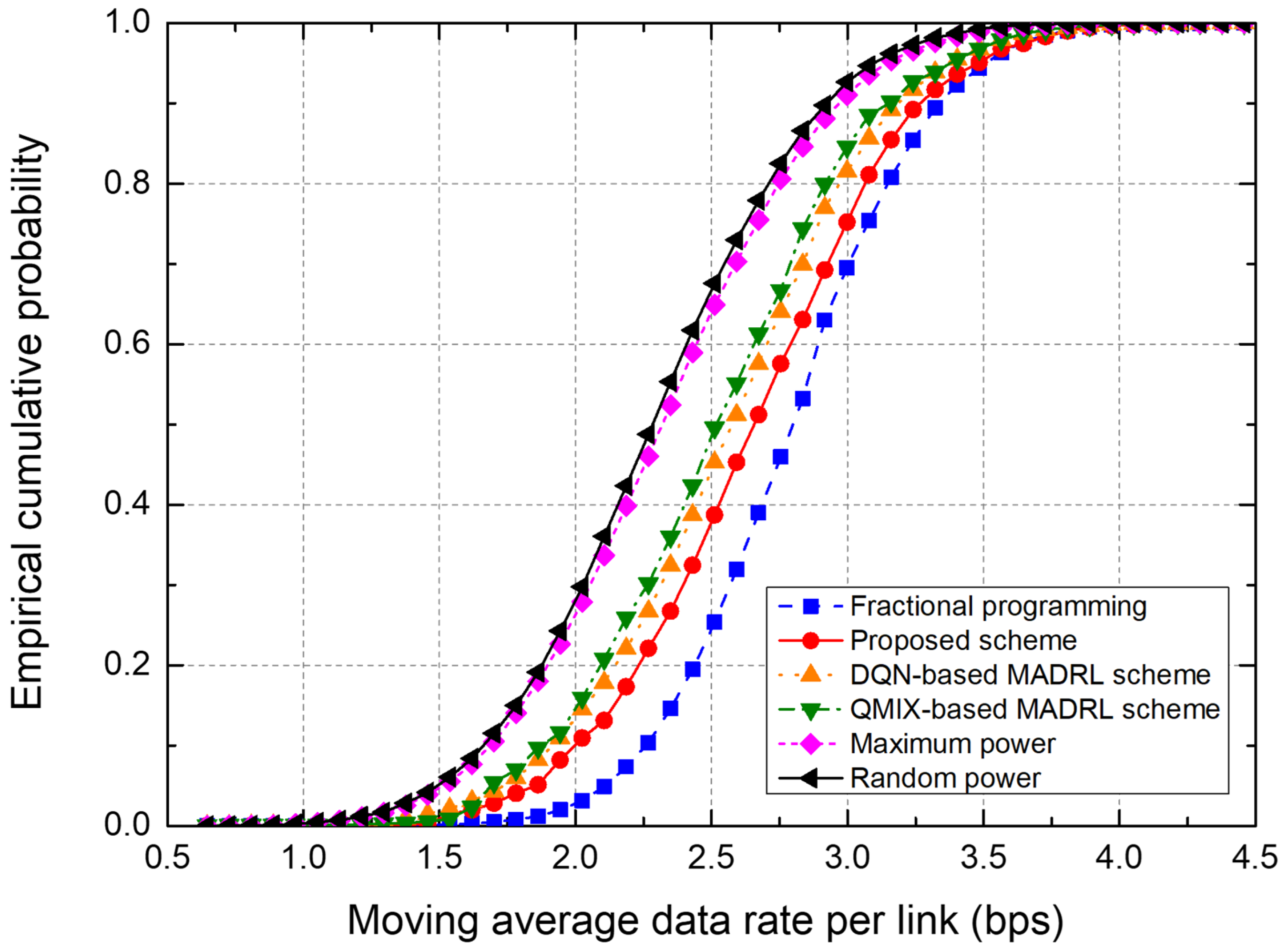
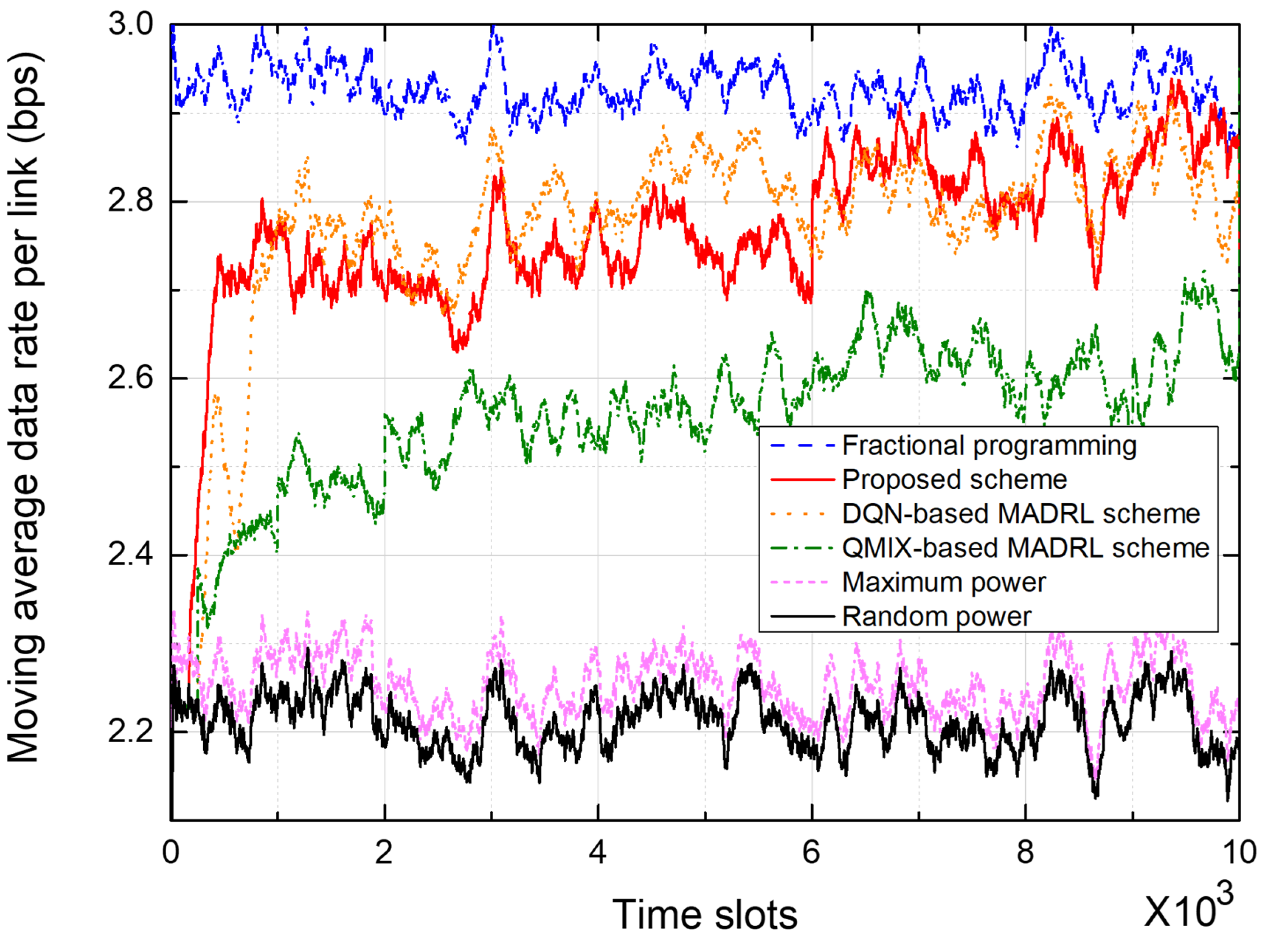
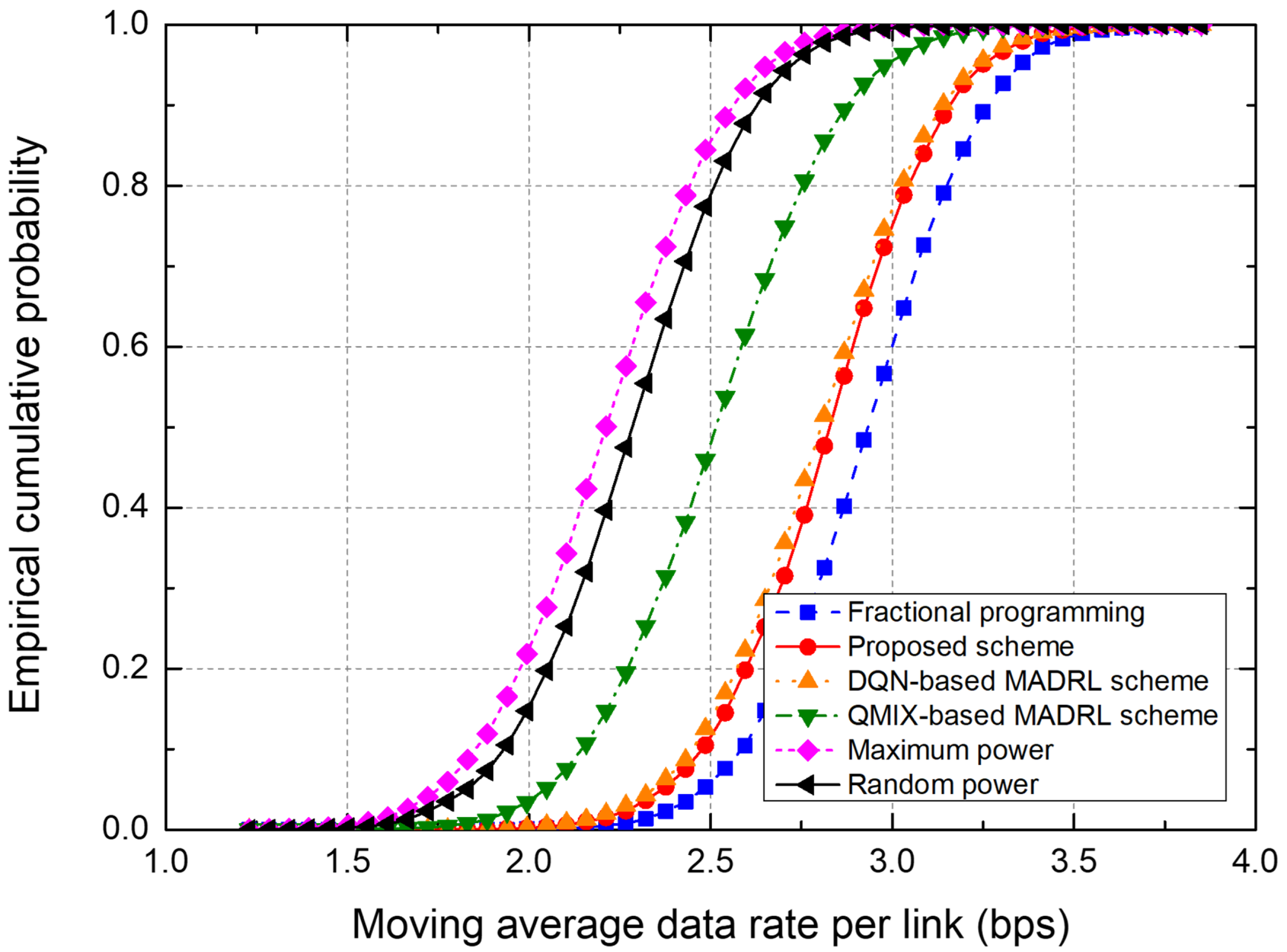
5.3. Average Data Rate Performance
5.4. Complexity Performance
6. Conclusions
Author Contributions
Funding
Data Availability Statement
Conflicts of Interest
References
- Xu, Y.; Gui, G.; Gacanin, H.; Adachi, F. A Survey on resource allocation for 5G heterogeneous networks: Current Research, future trends, and challenges. IEEE Commun. Surv. Tutor. 2021, 23, 668–695. [Google Scholar] [CrossRef]
- Lohan, P.; Kantarci, B.; Ferrag, M.A.; Tihanyi, N.; Shi, Y. From 5G to 6G networks: A survey on AI-based jamming and interference detection and mitigation. IEEE Open J. Commun. Soc. 2024, 5, 3920–3974. [Google Scholar] [CrossRef]
- Yi, M.; Yang, P.; Chen, M. A DRL-driven intelligent joint optimization strategy for computation offloading and resource allocation in ubiquitous edge IoT systems. IEEE Trans. Emerg. Top. Comput. Intell. 2023, 7, 39–54. [Google Scholar] [CrossRef]
- Agarwal, B.; Togou, M.A.; Marco, M.; Muntean, G.-M. A comprehensive survey on radio resource management in 5G hetNets: Current solutions, future trends and open issues. IEEE Commun. Surv. Tutor. 2022, 24, 2495–2534. [Google Scholar] [CrossRef]
- Hussain, F.; Hassan, S.A.; Hussain, R.; Hossain, E. Machine learning for resource management in cellular and IoT networks: Potentials, current solutions, and open challenges. IEEE Commun. Surv. Tutor. 2020, 22, 1251–1275. [Google Scholar] [CrossRef]
- Xiang, H.; Yang, Y.; He, G.; Huang, J.; He, D. Multi-agent deep reinforcement learning-based power control and resource allocation for D2D communications. IEEE Commun. Lett. 2022, 11, 1659–1663. [Google Scholar] [CrossRef]
- Giannopoulos, A.; Spantideas, S.; Capsalis, N.; Gkonis, P.; Karkazis, P.; Sarakis, L.; Trakadas, P.; Capsalis, C. WIP: Demand-driven power allocation in wireless networks with deep Q-learning. In Proceedings of the 2021 IEEE 22nd International Symposium on a World of Wireless, Mobile and Multimedia Networks (WoWMoM), Pisa, Italy, 7–11 July 2021; pp. 1–4. [Google Scholar]
- Zhu, H.; Wu, Q.; Wu, X. Wu, X.-J.; Fan, Q.; Fan, P.; Wang, J. Decentralized power allocation for MIMO-NOMA vehicular edge computing based on deep reinforcement learning. IEEE Internet Things J. 2022, 9, 12770–12782. [Google Scholar] [CrossRef]
- Ji, Z.; Qin, Z. Federated learning for distributed energy-efficient resource allocation. In Proceedings of the 2022 IEEE International Conference on Communications (ICC), Seoul, Republic of Korea, 16–20 September 2022; pp. 1–6. [Google Scholar]
- Wang, X.; Wang, S.; Liang, X.; Zhao, D.; Huang, J.; Xu, X.; Dai, B.; Miao, Q. Deep reinforcement learning: A survey. IEEE Trans. Neural Netw. Learn. Syst. 2024, 35, 5064–5078. [Google Scholar] [CrossRef] [PubMed]
- Bi, Z.; Zhou, W. Deep reinforcement learning based power allocation for D2D network. In Proceedings of the 2020 IEEE 91st Vehicular Technology Conference (VTC2020-Spring), Antwerp, Belgium, 25–28 May 2020; pp. 1–5. [Google Scholar]
- Luong, N.C.; Hoang, D.T.; Gong, S.; Niyato, D.; Wang, P.; Liang, Y.-C.; Kim, D.I. Applications of deep reinforcement learning in communications and networking: A survey. IEEE Commun. Surv. Tutor. 2019, 21, 3133–3174. [Google Scholar] [CrossRef]
- Meng, F.; Chen, P.; Wu, L.; Cheng, J. Power allocation in multi-user cellular networks: Deep reinforcement learning approaches. IEEE Trans. Wireless. Commun. 2020, 19, 6255–6267. [Google Scholar] [CrossRef]
- Wang, J.; Hong, Y.; Wang, J.; Xu, J.; Tang, Y.; Han, Q.-L.; Kurths, J. Cooperative and competitive multi-agent systems: From optimization to games. IEEE/CAA J. Autom. Sin. 2022, 9, 763–783. [Google Scholar] [CrossRef]
- Das, S.K.; Mudi, R.; Rahman, M.S.; Rabie, K.M.; Li, X. Federated reinforcement learning for wireless networks: Fundamentals, challenges and future research trends. IEEE Open J. Veh. Technol. 2024, 5, 1400–1440. [Google Scholar] [CrossRef]
- Lee, S.; Yu, H.; Lee, H. Multiagent Q-Learning-based multi-UAV wireless networks for maximizing energy efficiency: Deployment and power control strategy design. IEEE Internet Things J. 2022, 9, 6434–6442. [Google Scholar] [CrossRef]
- Kopic, A.; Perenda, E.; Gacanin, H. A collaborative multi-agent deep reinforcement learning-based wireless power allocation with centralized training and decentralized execution. IEEE Trans. Commun. 2024, 72, 7006–7016. [Google Scholar] [CrossRef]
- Dai, P.; Wang, H.; Hou, H.; Qian, X.; Yu, W. Joint spectrum and power allocation in wireless networks: A two-stage multi-agent reinforcement learning method. IEEE Trans. Emerg. Top. Comput. Intell. 2024, 8, 2364–2374. [Google Scholar] [CrossRef]
- Wang, Z.; Zong, J.; Zhou, Y.; Shi, Y.; Wong, V.W.S. Decentralized multi-agent power control in wireless networks with frequency reuse. IEEE Trans. Commun. 2021, 70, 1666–1681. [Google Scholar] [CrossRef]
- Park, C.; Kim, G.S.; Park, S.; Jung, S.; Kim, J. Multi-agent reinforcement learning for cooperative air transportation services in city-wide autonomous urban air mobility. IEEE Trans. Intell. Veh. 2023, 8, 4016–4030. [Google Scholar] [CrossRef]
- Nasir, Y.S.; Guo, D. Deep actor-critic learning for distributed power control in wireless mobile networks. In Proceedings of the 2020 54th Asilomar Conference on Signals Systems, and Computers, Pacific Grove, CA, USA, 1–4 November 2020; pp. 1–5. [Google Scholar]
- Yao, Y.; Zhou, H.; Erol-Kantarci, M. Deep reinforcement learning-based radio resource allocation and beam management under location uncertainty in 5G mm wave networks. In Proceedings of the 2022 IEEE Symposium on Computers and Communications (ISCC), Rhodes, Greece, 30 June–3 July 2022; pp. 1–6. [Google Scholar]
- Xu, Y.; Liy, X.; Zhou, W.; Yu, G. Generative adversarial LSTM networks learning for resource allocation in UAV-served M2M communications. IEEE Wirel. Commun. Lett. 2021, 26, 1601–1605. [Google Scholar] [CrossRef]
- Lin, Y.; Wang, M.; Zhou, X.; Ding, G.; Mao, S. Dynamic spectrum interaction of UAV flight formation communication with priority: A deep reinforcement learning approach. IEEE Trans. Cogn. Commun. Netw. 2020, 6, 892–903. [Google Scholar] [CrossRef]
- Sohaib, M.; Jeong, J.; Jeon, S.-W. Dynamic multichannel access via multi-agent reinforcement learning: Throughput and fairness guarantees. IEEE Trans. Wirel. Commun. 2021, 21, 3994–4008. [Google Scholar] [CrossRef]
- Shi, Q.; Razaviyayn, M.; Luo, Z.-Q.; He, C. An iteratively weighted MMSE approach to distributed sum-utility maximization for a MIMO interfering broadcast channel. IEEE Trans. Signal Process. 2011, 59, 4331–4340. [Google Scholar] [CrossRef]
- Shen, K.; Yu, W. Fractional programming for communication systems—Part I: Power control and beamforming. IEEE Trans. Signal Process. 2018, 66, 2616–2630. [Google Scholar] [CrossRef]
- Ahmad, I.; Becvar, Z.; Mach, P. Coordinated machine learning for channel reuse and transmission power allocation for D2D communication. In Proceedings of the IEEE Global Communications Conference, Cape Town, South Africa, 8–12 December 2024; pp. 2701–2706. [Google Scholar]
- Lee, W.; Kim, M.; Cho, D.-H. Deep power control: Transmit power control scheme based on convolutional neural network. IEEE Commun. Lett. 2018, 22, 1276–1279. [Google Scholar] [CrossRef]
- Shen, Y.; Yuanming, S.; Zhang, J.; Letaief, K. Graph neural networks for scalable radio resource management: Architecture design and theoretical analysis. IEEE J. Sel. Areas Commun. 2021, 39, 101–115. [Google Scholar] [CrossRef]
- Han, D.; So, J. Energy-Efficient Resource Allocation Based on Deep Q-Network in V2V Communications. Sensors 2023, 23, 1295. [Google Scholar] [CrossRef] [PubMed]
- Lee, L.; Kim, H.; So, J. Reinforcement Learning-Based Joint Beamwidth and Beam Alignment Interval Optimization in V2I Communications. Sensors 2024, 24, 837. [Google Scholar] [CrossRef]
- Zhao, G.; Li, Y.; Xu, C.; Han, Z.; Xing, Y.; Yu, S. Joint power control and channel allocation for interference mitigation based on reinforcement learning. IEEE Access 2019, 7, 177254–177265. [Google Scholar] [CrossRef]
- Nasir, Y.S.; Guo, D. Multi-agent deep reinforcement Learning for dynamic power allocation in wireless networks. IEEE J. Sel. Areas Commun. 2019, 37, 2239–2250. [Google Scholar] [CrossRef]
- Zhou, Y.; Zhuang, W. Throughput analysis of cooperative communication in wireless ad hoc networks with frequency reuse. IEEE Trans. Wirel. Commun. 2014, 14, 205–218. [Google Scholar] [CrossRef]
- Liang, L.; Kim, J.; Jha, S.C.; Sivanesan, K.; Li, G.Y. Spectrum and power allocation for vehicular communications with delayed CSI feedback. IEEE Commun. Lett. 2017, 6, 458–461. [Google Scholar] [CrossRef]
- Technical Specification Group Radio Access Network; Radio Frequency (RF) System Scenarios (Release 18), Document 3GPP TR 25.942 V18.0.0, 3rd Generation Partnership Project. March 2024. Available online: https://www.3gpp.org/ftp/Specs/archive/25_series/25.942/25942-i00.zip (accessed on 1 November 2024).
- Luo, Z.-Q.; Zhang, S. Dynamic spectrum management: Complexity and duality. IEEE J. Sel. Top. Signal Process. 2008, 2, 57–73. [Google Scholar]
- Majid, A.Y.; Saaybi, S.; Francois-Lavet, V.; Prasad, R.V.; Verhoeven, C. Deep reinforcement learning versus evolution strategies: A comparative survey. IEEE Trans. Neural Netw. Learn. Syst. 2023, 35, 11939–11957. [Google Scholar] [CrossRef] [PubMed]
- Rosenberger, J.; Urlaub, M.; Rauterberg, F.; Lutz, T.; Selig, A.; Bühren, M.; Schramm, D. Deep reinforcement learning multi-agent system for resource allocation in industrial internet of things. Sensors 2022, 22, 4099. [Google Scholar] [CrossRef] [PubMed]
- Zhao, X.; Zhang, Y.A. Joint beamforming and scheduling for integrated sensing and communication systems in URLLC: A POMDP approach. IEEE Trans. Commun. 2024, 72, 6145–6161. [Google Scholar] [CrossRef]
- IEEE Std 754-2019 (Revision of IEEE 754-2008); IEEE Standard for Floating-Point Arithmetic. IEEE: New York, NY, USA, 2019; pp. 1–84.
- Liu, K.; Li, L.; Zhang, X. Fast and accurate identification of kiwifruit diseases using a lightweight convolutional neural network architecture. IEEE Access 2025, 13, 84826–84843. [Google Scholar] [CrossRef]
- Mhatre, S.; Adelantado, F.; Ramantas, K.; Verikoukis, C. Intelligent QoS-aware slice resource allocation with user association parameterization for beyond 5G O-RAN-based architecture using DRL. IEEE Trans. Veh. Technol. 2025, 74, 3096–3109. [Google Scholar] [CrossRef]


| Symbol | Description |
|---|---|
| The set of BS indices | |
| K | The number of BSs |
| The user served by BS k in time slot t | |
| The downlink channel gain from BS k to user in time slot t | |
| The small-scale fading from BS k to user in time slot t | |
| The channel innovation process from BS k to user in time slot t | |
| The correlation coefficient | |
| The maximum Doppler frequency (Hz) | |
| T | The slot duration |
| The large-scale fading component from BS k to user in time slot t | |
| The shadow-fading component in time slot t (dB) | |
| The shadowing standard deviation (dB) | |
| The additive white Gaussian noise (AWGN) power spectral density | |
| The shadow channel innovation process from BS k to user | |
| The received SINR of user k at time slot t (dB) | |
| The downlink transmit power set in time slot t | |
| The transmit power of BS k in time slot t (dBm) |
| Parameter | Value |
|---|---|
| Number of cells | |
| Maximum transmit power | 30 dBm |
| Pathloss model | 3GPP TR 25.942 |
| Slot duration, T | 20 ms |
| Number of slots in simulation | 10,000 slots |
| Carrier frequency | 2 GHz |
| Frequency bandwidth | 10 MHz |
| Shadowing distribution, | Log-normal, 8 dB |
| Maximum Doppler frequency, | 10 Hz |
| Noise power spectral density, | dBm |
| Parameter | Value |
|---|---|
| Number of training episodes | 100 |
| Number of neurons in the encoder | 128 |
| Number of neurons in the actor LSTM | 32 |
| Number of neurons in the critic LSTM | 64 |
| Number of neurons in the decoder | 128 |
| Actor optimizer | Adam |
| Critic optimizer | Adam |
| Actor learning rate, | |
| Critic learning rate, | |
| Soft update parameter, | |
| Reward discount factor, | |
| Loss function | Clipped MSE |
| Model | 7-Cell Network | 19-Cell Network | ||
|---|---|---|---|---|
| # of Parameters | # of MACs | # of Parameters | # of MACs | |
| DQN-based scheme | 36,150 | 250,600 | 36,150 | 680,200 |
| QMIX-based scheme | 931,990 | 927,744 | 2,358,970 | 2,348,544 |
| Proposed scheme | 208,424 | 567,392 | 464,564 | 1,540,064 |
Disclaimer/Publisher’s Note: The statements, opinions and data contained in all publications are solely those of the individual author(s) and contributor(s) and not of MDPI and/or the editor(s). MDPI and/or the editor(s) disclaim responsibility for any injury to people or property resulting from any ideas, methods, instructions or products referred to in the content. |
© 2025 by the authors. Licensee MDPI, Basel, Switzerland. This article is an open access article distributed under the terms and conditions of the Creative Commons Attribution (CC BY) license (https://creativecommons.org/licenses/by/4.0/).
Share and Cite
Kim, H.; So, J. Distributed Multi-Agent Deep Reinforcement Learning-Based Transmit Power Control in Cellular Networks. Sensors 2025, 25, 4017. https://doi.org/10.3390/s25134017
Kim H, So J. Distributed Multi-Agent Deep Reinforcement Learning-Based Transmit Power Control in Cellular Networks. Sensors. 2025; 25(13):4017. https://doi.org/10.3390/s25134017
Chicago/Turabian StyleKim, Hun, and Jaewoo So. 2025. "Distributed Multi-Agent Deep Reinforcement Learning-Based Transmit Power Control in Cellular Networks" Sensors 25, no. 13: 4017. https://doi.org/10.3390/s25134017
APA StyleKim, H., & So, J. (2025). Distributed Multi-Agent Deep Reinforcement Learning-Based Transmit Power Control in Cellular Networks. Sensors, 25(13), 4017. https://doi.org/10.3390/s25134017