

An Iterative Error Correction Procedure for Single Sheet Testers Using FEM 3D Model


Abstract
1. Introduction
2. Core Loss Models
- Steinmetz equation-based models.
- Loss separation-based models.
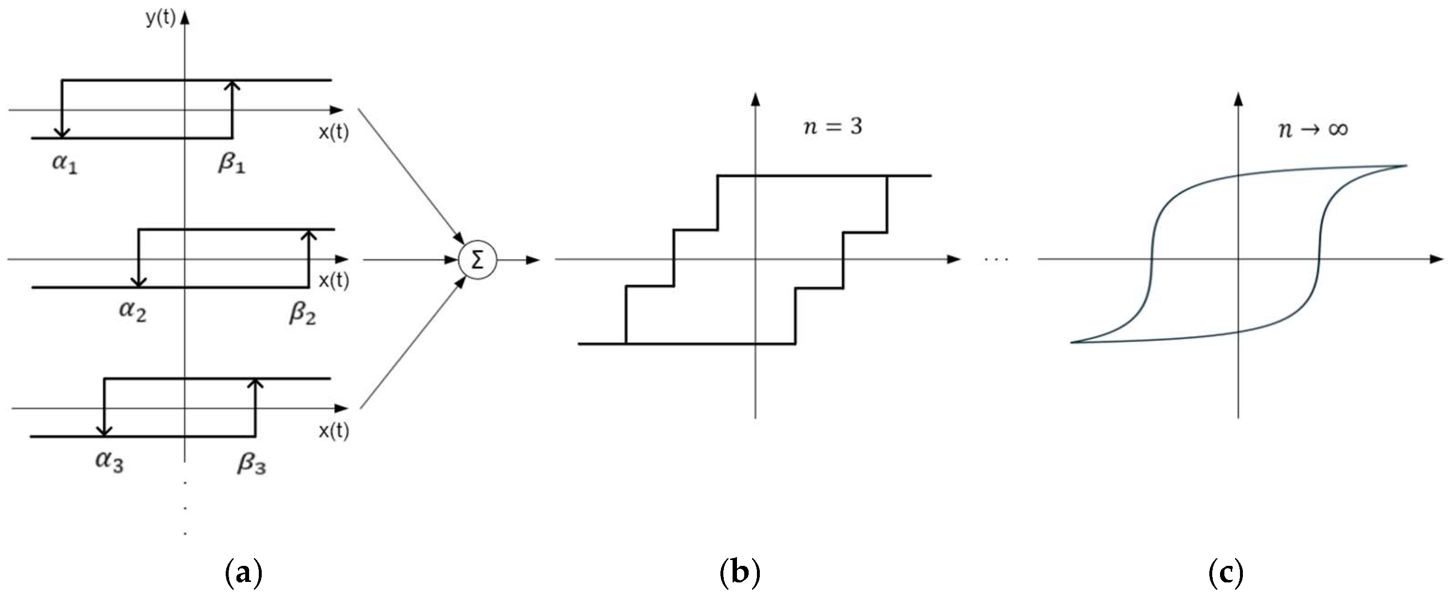
- Mathematical hysteresis-based models.
2.1. Steinmetz Equation-Based Models
2.2. Loss Separation Models
2.3. Core Loss Calculation in ANSYS Maxwell
3. BH Curve Models
- -
- The model has to be continuously differentiable
- -
- -
- for every s
- -
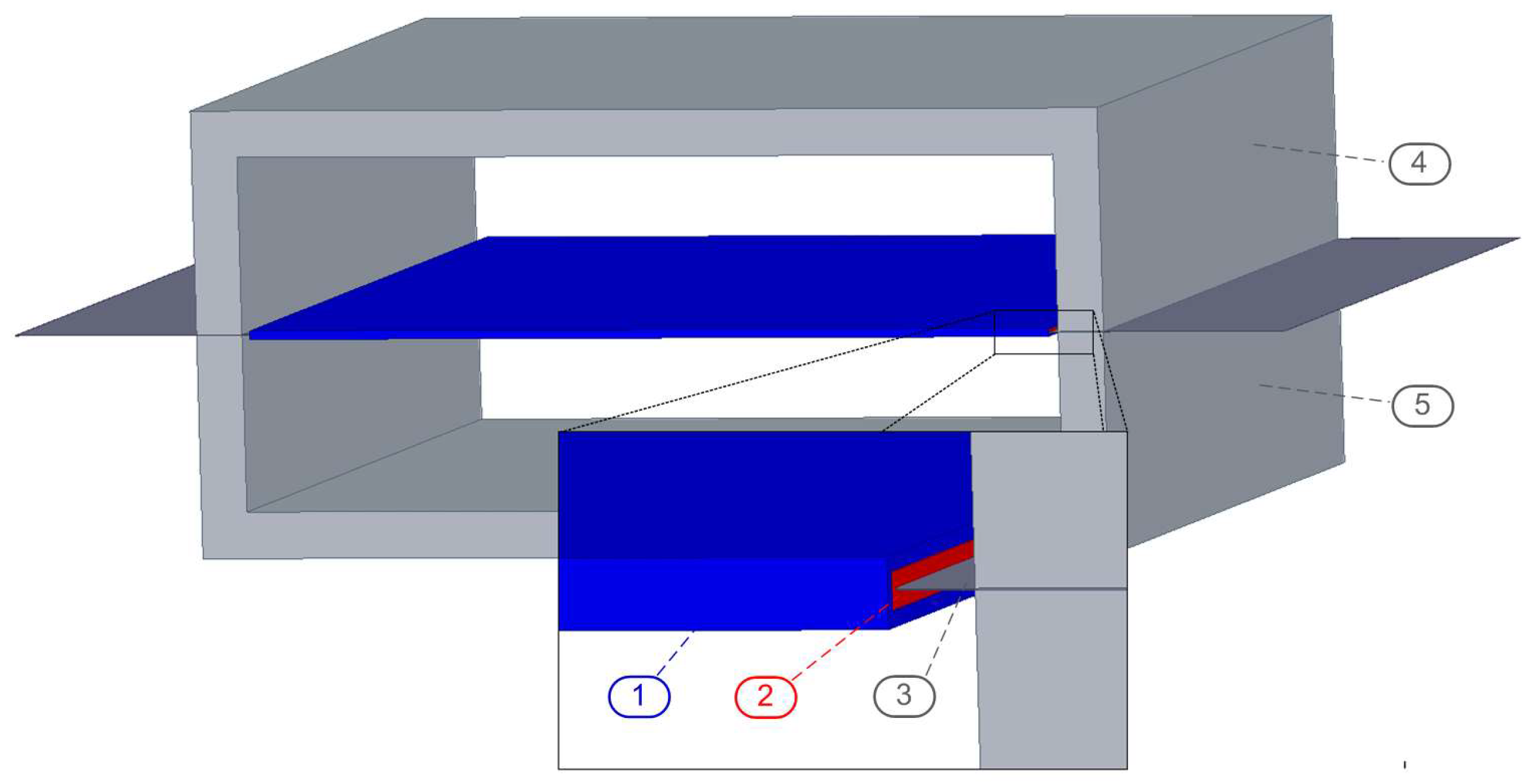
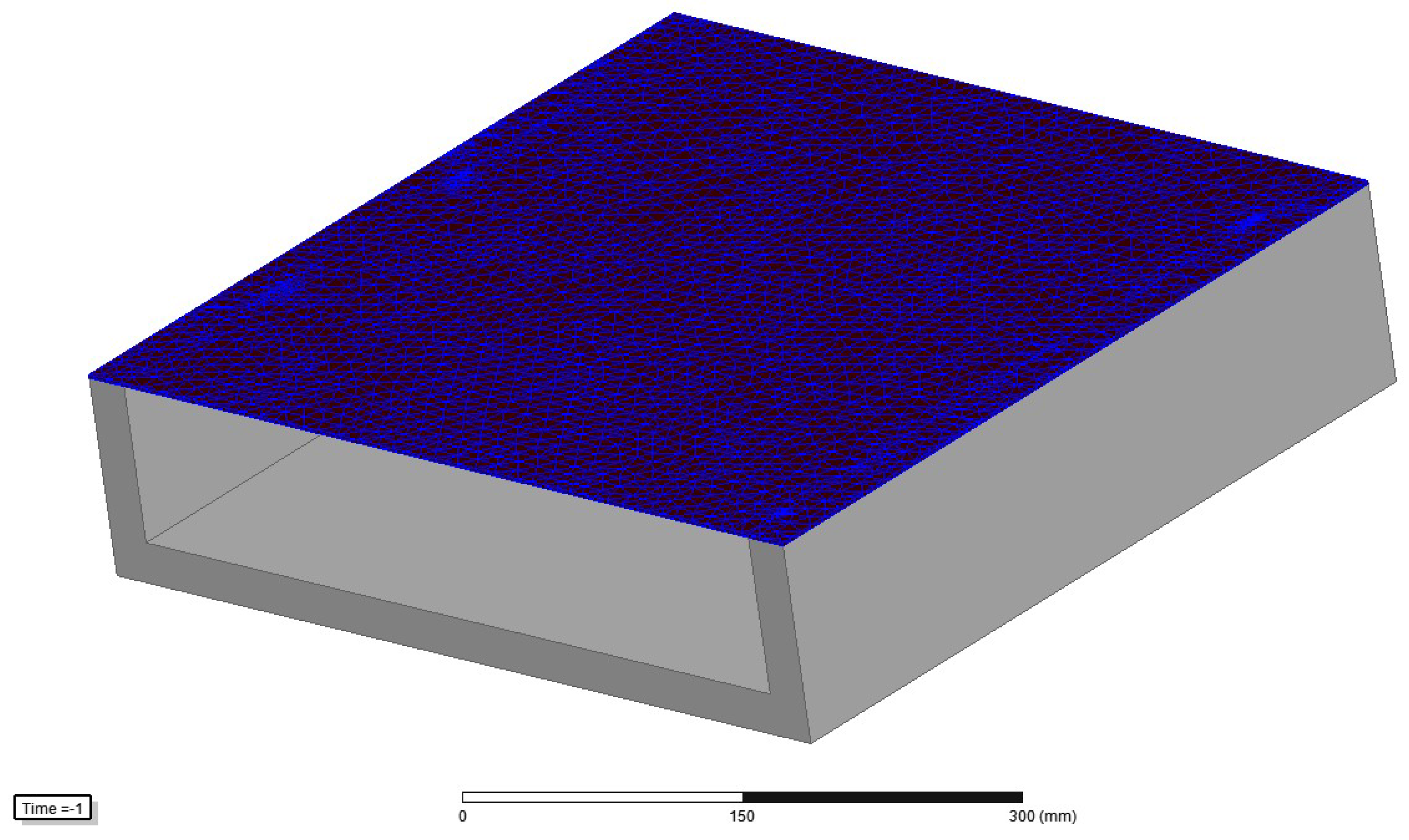
4. Simulation Setup of the 3D SST Model
4.1. Specifications of the SST 3D Model
- (a)
- Yoke specifications:
- -
- Pole face width: 25 mm ± 1 mm
- -
- Coplanarity of pole faces: Within 0.5 mm
- -
- Gap between opposite pole faces: Not exceeding 0.005 mm
- -
- Yoke height: 90 mm to 150 mm
- -
- Yoke width: 500 mm ± 55 mm
- -
- Inside length of yoke: 450 mm ± 1 mm
- (b)
- Windings specifications
- -
- Minimum length: 440 mm
- -
- Former dimensions
- -
- Length: 445 mm ± 2 mm
- -
- Internal width: 510 mm ± 1 mm
- -
- Internal height: 5 mm (−0/+2 mm)
- -
- Height: ≤15 mm
- (c)
- Primary winding options:
- -
- Multiple coils: Identical coils with identical turns and connected in parallel
- -
- Single continuous winding: Spanning the full length
Note: Secondary winding turn number is based on the measurement device. - (d)
- Test specimen specifications:
- -
- Length: ≥500 mm
- -
- Width: As wide as possible (minimum 60% of yoke width)
- -
- Cutting tolerances:
- -
- Grain-oriented steel: ±1°
- -
- Non-oriented steel: ±5°
Note: Specimens must be free of burrs, flat, and without mechanical distortions. - (e)
- Power supply requirements:
- -
- Voltage and frequency stability: ±0.2%
- -
- Waveform: Should be sinusoidal with a form factor of 1.111 ± 1%
Note: A stable power supply with low internal impedance is required.
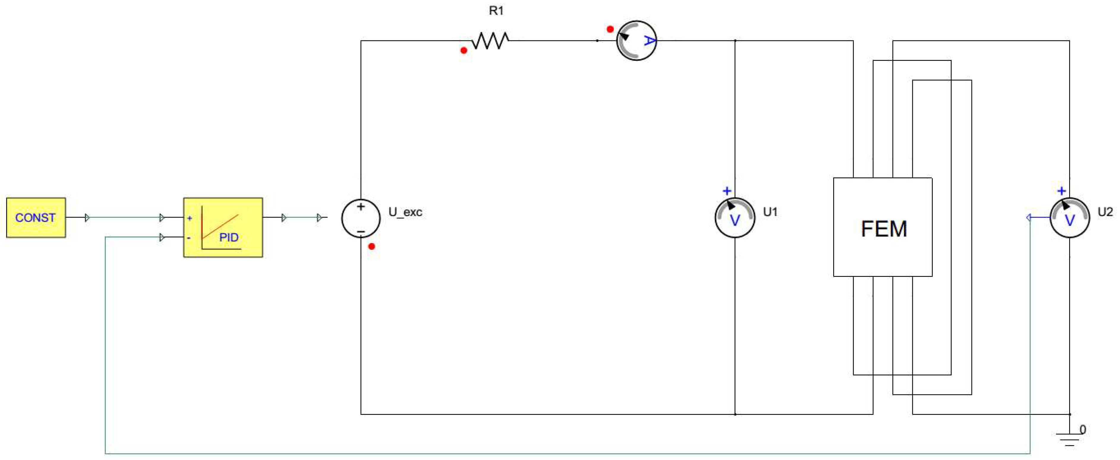
4.2. Simplorer Model with Transient Co-Simulation
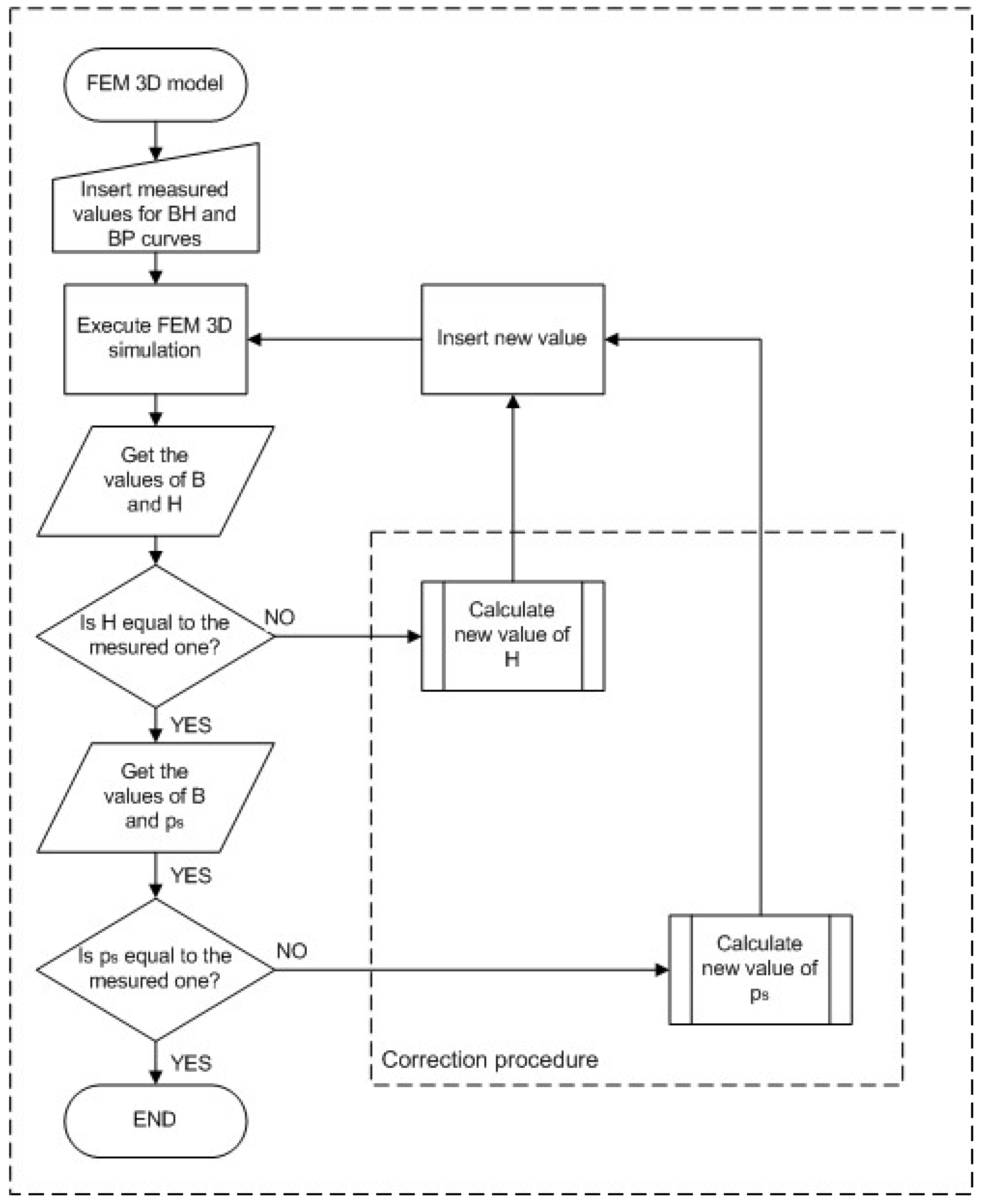
5. Proposed Iterative Procedure for Error Correction
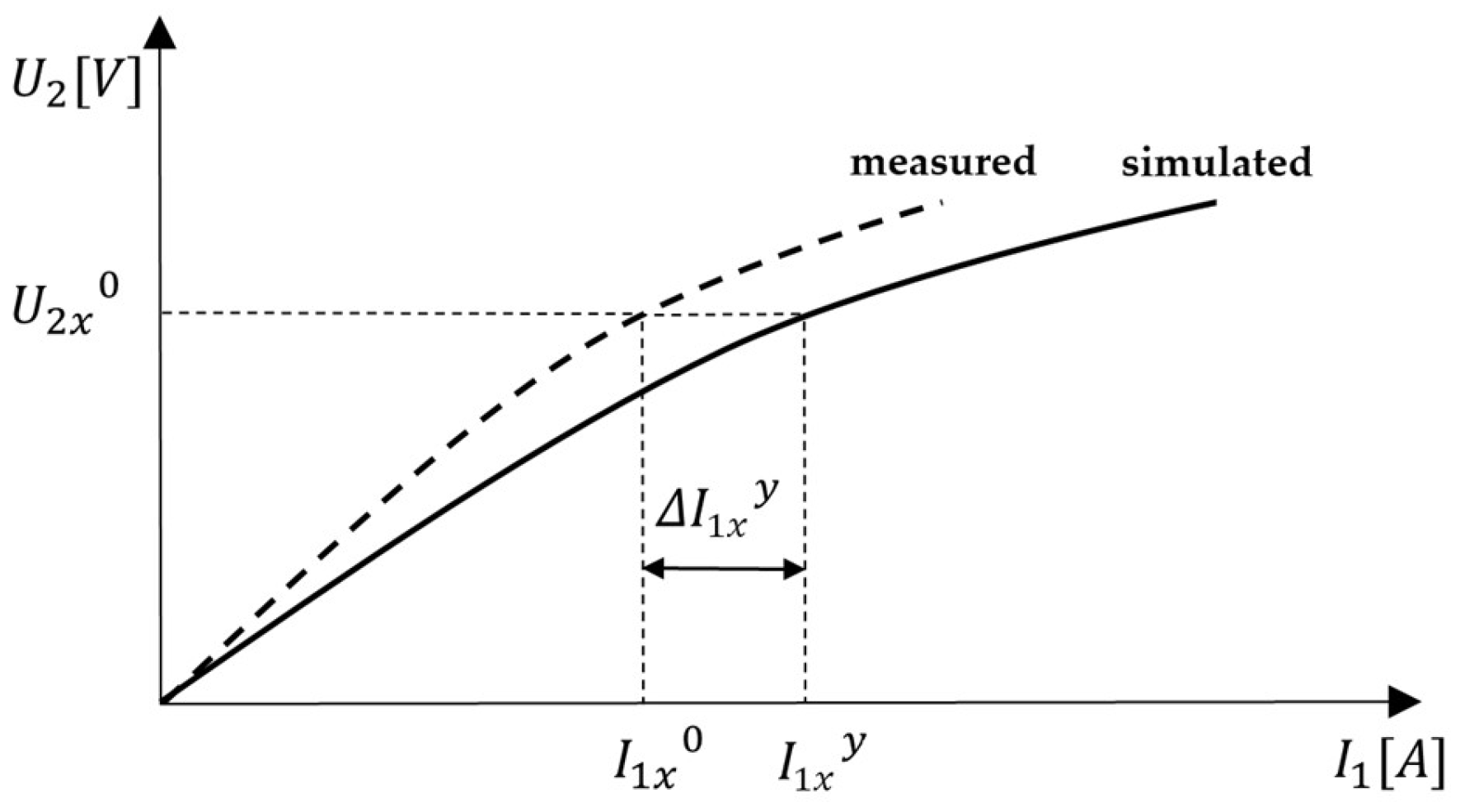
5.1. Steepest Descent Method and Gradient Estimation
5.2. Error Correction Method for BH Curve
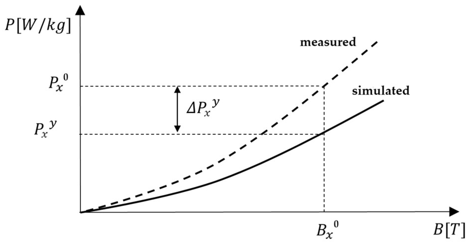
5.3. Error Correction Method for PB Curve
6. Results
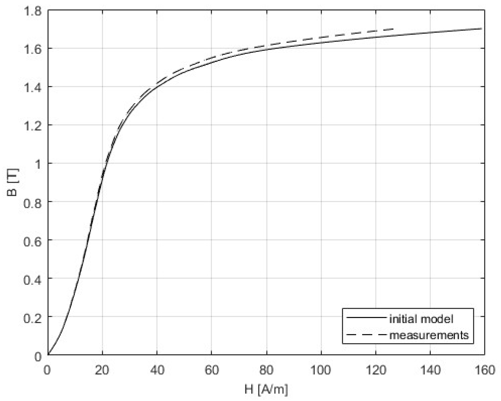
6.1. Measurements
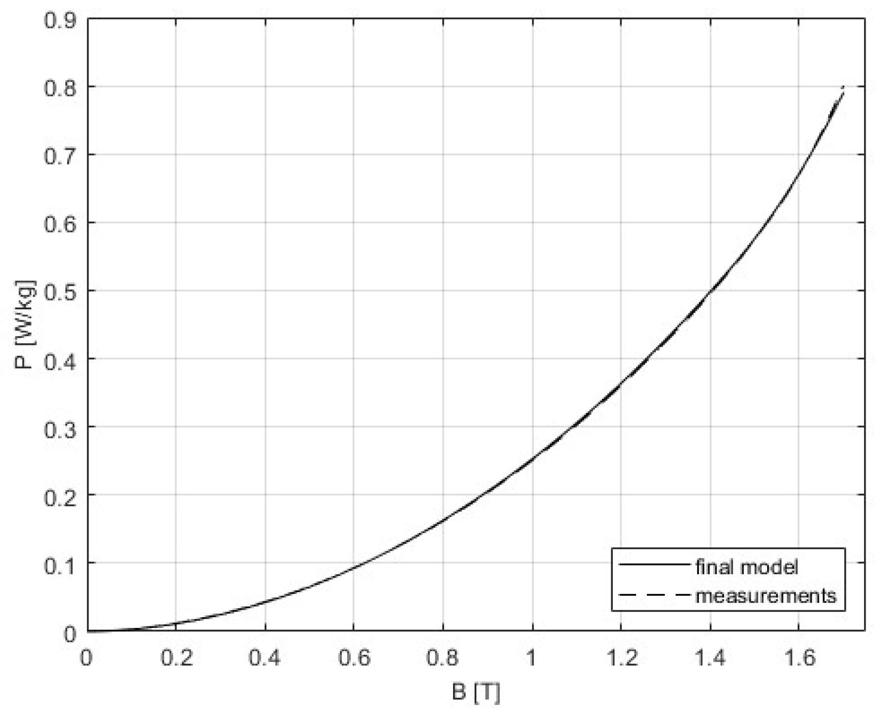
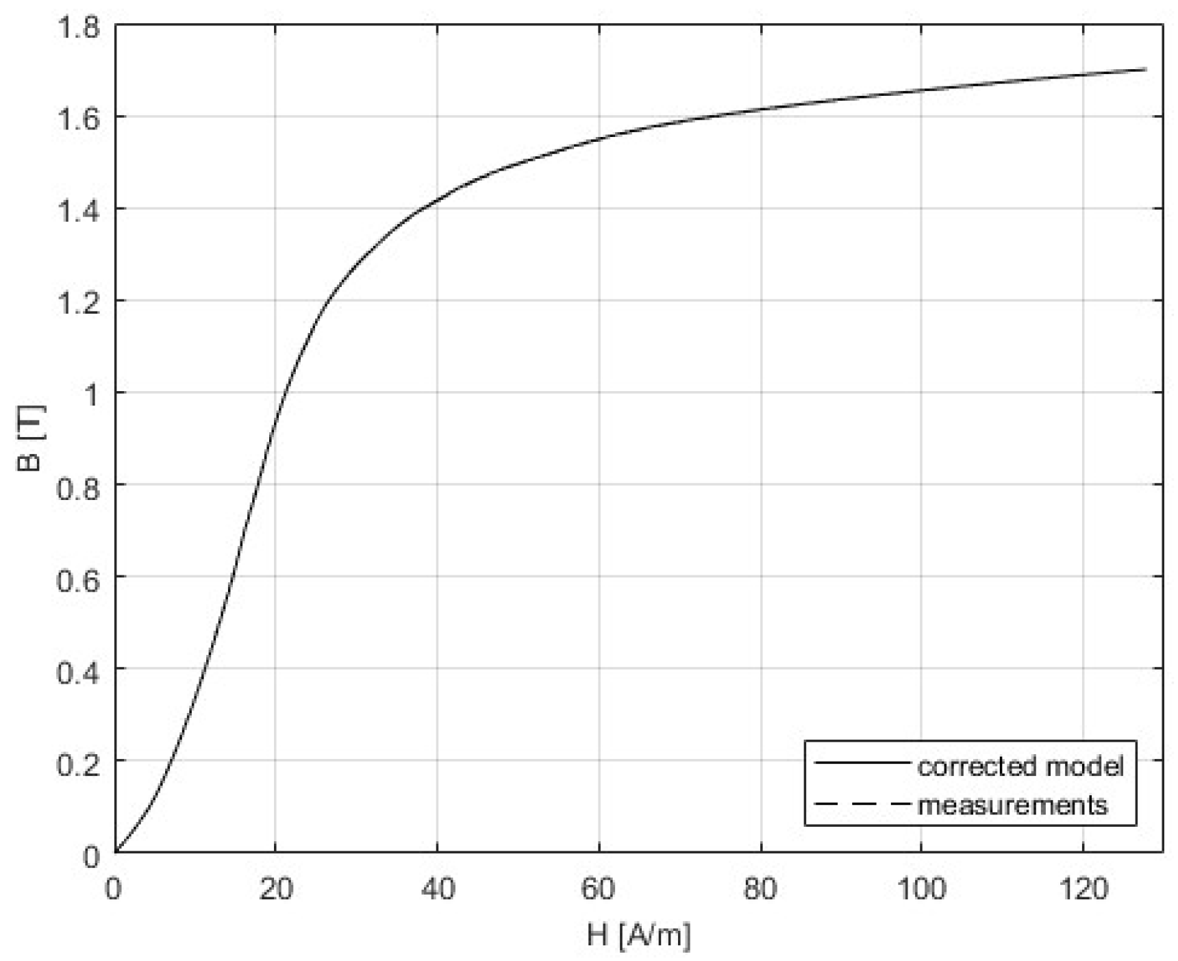
6.2. Corrected Curves
7. Discussion and Conclusions
Author Contributions
Funding
Institutional Review Board Statement
Informed Consent Statement
Data Availability Statement
Conflicts of Interest
References
- Levi, E. Polyphase Motors: A Direct Approach to their Design; John Wiley & Sons: London, UK, 1984. [Google Scholar]
- Derbas, H.W.; Williams, J.M.; Koenig, A.C.; Pekarek, S.D. A Comparison of Nodal- and Mesh-Based Magnetic Equivalent Circuit Models. IEEE Trans. Energy Convers. 2009, 24, 388–396. [Google Scholar] [CrossRef]
- Horvath, D.C.; Pekarek, S.D.; Sudhoff, S.D. A Scaled Mesh/Nodal Formulation of Magnetic Equivalent Circuits With Motion. IEEE Trans. Energy Convers. 2019, 34, 58–69. [Google Scholar] [CrossRef]
- Bash, M.L.; Pekarek, S. Analysis and Validation of a Population-Based Design of a Wound-Rotor Synchronous Machine. IEEE Trans. Energy Convers. 2012, 27, 603–614. [Google Scholar] [CrossRef]
- Elloumi, D.; Ibala, A.; Rebhi, R.; Masmoudi, A. Lumped Circuit Accounting for the Rotor Motion Dedicated to the Investigation of the Time-Varying Features of Claw Pole Topologies. IEEE Trans. Magn. 2015, 51, 1–8. [Google Scholar] [CrossRef]
- IEEE Std 393–1991; IEEE Standard Procedures for Magnetic Cores. IEEE: Piscataway, NJ, USA, 1992.
- IEC Standard 60404–2; Methods of Measurement of the Magnetic Properties of Electrical Steel Sheet and Strip by Means of an Epstein Frame. IEC: Geneva, Switzerland, 1996.
- Pfützner, H.; Shilyashki, G. Theoretical Basis for Physically Correct Measurement and Interpretation of Magnetic Energy Losses. IEEE Trans. Magn. 2018, 54, 1–7. [Google Scholar] [CrossRef]
- IEC Standard 60404–3; Methods of Measurement of the Magnetic Properties of Electrical Steel Strip and Sheet by Means of a Single Sheet Tester. IEC: Geneva, Sriwitzerland, 2022.
- Yamamoto, T.; Ohya, Y. Single sheet tester for measuring core losses and permeabilities in a silicon steel sheet. IEEE Trans. Magn. 1974, 10, 157–159. [Google Scholar] [CrossRef]
- Gmyrek, Z. Single Sheet Tester with Variable Dimensions. IEEE Trans. Instrum. Meas. 2016, 65, 1661–1668. [Google Scholar] [CrossRef]
- Antonelli, E.; Cardelli, E.; Faba, A. Epstein frame: How and when it can be really representative about the magnetic behavior of laminated magnetic steels. IEEE Trans. Magn. 2005, 41, 1516–1519. [Google Scholar] [CrossRef]
- Moses, A.; Hamadeh, S. Comparison of the Epstein-square and a single-strip tester for measuring the power loss of nonoriented electrical steels. IEEE Trans. Magn. 1983, 19, 2705–2710. [Google Scholar] [CrossRef]
- Németh, S.; Hargitai, C.; Szabó, L.; Papp, L. Field and loss measurements in Epstein frame and sheet testers. J. Magn. Magn. Mater. 1996, 160, 183–184. [Google Scholar] [CrossRef]
- Cassat, A.; Espanet, C.; Wavre, N. BLDC motor stator and rotor iron losses and thermal behavior based on lumped s chemes and 3 3-D FEM analysis. IEEE Trans. Ind. Appl. 2003, 39, 1314–1322. [Google Scholar] [CrossRef]
- Hyuk, N.; Kyung-Ho, H.K.; Jeong-Jong, L.J.; Jung-Pyo, H.J.; Gyu-Hong, K.G. A study on iron loss analysis method considering the harmonics of the flux density waveform using iron loss cur ves tested on epstein samples. IEEE Trans. Magn. 2003, 39, 1472–1475. [Google Scholar] [CrossRef]
- Wang, X.; Xie, D.; Cheng, Z.; Zhang, J. Loss Analysis of Transformer Core using FEM Method Taking Account of Anisotropy. In Proceedings of the 2008 International Conference on Electrical Machines and Systems, Wuhan, China, 17–20 October 2008; pp. 485–488. [Google Scholar]
- Leonardi, F.; Matsuo, T.; Lipo, T.A. Iron Loss Calculation for Synchronous Reluctance Machines. In Proceedings of the IEEE International Conference on Power Electronics, Drives & Energy Systems for Industrial Growth, New Delhi, India, 8–11 January 1996. [Google Scholar]
- Li, Y.; Zhu, L.; Zhu, J. Calculation of Core Losses Under DC Bias and Harmonics Based on Jiles-Atherton dynamic Hysteresis Model Combined with Finite Element Analysis. In Proceedings of the 2017 20th International Conference on Electrical Machines and Systems (ICEMS), Sydney, NSW, Australia, 11–14 August 2017; pp. 1–5. [Google Scholar] [CrossRef]
- Shah, S.B.; Rasilo, P.; Belahcen, A.; Arkkio, A. Experimental and Theoretical Study Of interlaminar Eddy Current Loss in Laminated Cores. In Proceedings of the 2017 20th International Conference on Electrical Machines and Systems (ICEMS), Sydney, NSW, Australia, 11–14 August 2017; pp. 1–6. [Google Scholar] [CrossRef]
- Abeywickrama, K.G.N.B.; Daszczynski, T.; Serdyuk, Y.V.; Gubanski, S.M. Determination of Complex Permeability of Silicon Steel for Use in High-Frequency Modeling of Power Transformers. IEEE Trans. Magn. 2008, 44, 438–444. [Google Scholar] [CrossRef]
- Abdallh, A.A.-E.; Sergeant, P.; Crevecoeur, G.; Vandenbossche, L.; Dupre, L.; Sablik, M. Magnetic Material Identification in Geometries With Non-Uniform Electromagnetic Fields Using Global and Local Magnetic Measurements. IEEE Trans. Magn. 2009, 45, 4157–4160. [Google Scholar] [CrossRef]
- Abdallh, A.A.-E.; Sergeant, P.; Crevecoeur, G.; Dupre, L. An Inverse Approach for Magnetic Material Characterization of an EI Core Electromagnetic Inductor. IEEE Trans. Magn. 2010, 46, 622–625. [Google Scholar] [CrossRef]
- Abdallh, A.A.-E.; Sergeant, P.; Dupre, L. A Non-Destructive Methodology for Estimating the Magnetic Material Properties of an Asynchronous Motor. IEEE Trans. Magn. 2012, 48, 1621–1624. [Google Scholar] [CrossRef]
- Rygal, R.; Moses, A.J.; Derebasi, N.; Schneider, J.; Schoppa, A. Influence of cutting stress on magnetic field and flux density distribution in non-oriented electrical steels. J. Magn. Magn. Mater. 2000, 215, 687–689. [Google Scholar] [CrossRef]
- Schoppa, A.; Schneider, J.; Wuppermann, C.D. Influence of the manufacturing process on the magnetic properties of non-oriented electrical steels. J. Magn. Magn. Mater. 2000, 215, 74–78. [Google Scholar] [CrossRef]
- Schoppa, A.; Schneider, J.; Wuppermann, C.D.; Bakon, T. Influence of welding and sticking of laminations on the magnetic properties of non-oriented electrical steels. J. Magn. Magn. Mater. 2003, 254–255, 367–369. [Google Scholar] [CrossRef]
- Reinlein, M.; Regnet, M.; Szary, P.; Abele, U.; Kremser, A. Impact of Different Cutting Methods on Core Losses and Magnetizing Demand of Electrical Steel Sheets. In Proceedings of the IKMT 2019-Innovative small Drives and Micro-Motor Systems, 12. ETG/GMM-Symposium. Wuerzburg, Germany, 10–11 September 2019; pp. 1–5. [Google Scholar]
- Steinmetz, C.P. On the Law of Hysteresis. J. Exp. Anal. Behav. 1984, 13, 243–266. [Google Scholar] [CrossRef]
- Reinert, J.; Brockmeyer, A.; De Doncker, R.W.A.A. Calculation of losses in ferro and ferrimagnetic materials based on the modified Steinmetz equation. IEEE Trans. Ind. Appl. 2001, 37, 1055–1061. [Google Scholar] [CrossRef]
- Ortigoza, M.A. Theoretical Studies of Electronic, Vibrational, and Magnetic Properties of Chemisorbed Surfaces and Nanoalloys; ProQuest: Ann Arbor, MI, USA, 2007. [Google Scholar]
- Li, J.L.J.; Abdallah, T.; Sullivan, C.R. Improved calculation of core loss with nonsinusoidal waveforms. IEEE Ind. Appl. Conf. 2001, 4, 2203–2210. [Google Scholar]
- Krings, A.; Soulard, J. Overview and Comparison of Iron Loss Models for Electrical Machines. J. Electr. Eng. 2010, 10, 162–169. [Google Scholar]
- Venkatachalam, K.; Sullivan, C.R.R.; Abdallah, T.; Tacca, H.; Waveforms, N.; Only, U.; Sullivan, C.R.R.; Abdallah, T.; Tacca, H. Accurate Prediction of Ferrite Core loss with Nonsinusoidal Waveforms using Only Steinmetz Parameters. In Proceedings of the 2002 IEEE Workshop on Computers in Power Electronics, Mayagüez, Portada, 3–4 June 2002; pp. 36–41. [Google Scholar]
- Van Den Bossche, A.; Valchev, V.C.; Georgiev, G.B. Measurement and loss model of ferrites with non-sinusoidal waveforms. PESC Rec. IEEE Annu. Power Electron. Spec. Conf. 2004, 6, 4814–4818. [Google Scholar]
- Femia, N.; Di Capua, G.; Oliva, N.; De Guglielmo, L. Performance-Based Experimental Characterization and Maximum Efficiency Point Detection of Power Inductors. IEEE Trans. Power Electron. 2025, 40, 1532–1541. [Google Scholar] [CrossRef]
- Krings, A. Iron Losses in Electrical Machines—Influence of Material Properties, Manufacturing Processes, and Inverter Operation; KTH Royal Institute of Technology: Stockholm, Sweden, 2014. [Google Scholar]
- Bertotti, G.; Di Schino, G.; Milone, A.F.; Fiorillo, F. On the effect of grain size on magnetic losses of 3% non-oriented SiFe. Le J. Phys. Colloq. 1985, 46, 385–388. [Google Scholar]
- Fiorillo, F.; Novikov, A. An improved approach to power losses in magnetic laminations under non sinusoidal induction waveform. IEEE Trans. Magn. 1990, 26, 2904–2910. [Google Scholar] [CrossRef]
- Bertotti, G. General Properties of Power Losses in Soft Ferromagnetic Materials. IEEE Trans. Magn. 1988, 24, 621–630. [Google Scholar] [CrossRef]
- Pluta, W.A. Some Properties of Factors of Specific Total Loss Components in Electrical Steel. IEEE Trans. Magn. 2010, 46, 322–325. [Google Scholar] [CrossRef]
- Bertotti, G.; Fiorillo, F.; Soardo, G.P. The prediction of power losses in soft magnetic materials. Le J. Phys. Colloq. 1988, 49, 1915–1919. [Google Scholar]
- ANSYS Inc. Maxwell Online Help, Version 17.2; Section 10: Assigning Materials, Paragraph: Calculating Properties for Core Loss (BP Curve), p. 22. ANSYS Electromagnetics Suite 17.2. Available via the Help menu in ANSYS Maxwell software by selecting “Maxwell PDF”. Available online: https://www.ansys.com/products/electronics/ansys-maxwell (accessed on 13 March 2024).
- Yuan, J.; Li, X.; Zhou, H.; Muramatsu, K. Modeling and Calculation of Core Loss and Heat Distribution in Ultra-Thin Wound Core Reactor Based on Electromagnetic and Fluid-Thermal Coupling. IEEE Trans. Magn. 2025. [Google Scholar] [CrossRef]
- Barg, S.; Barg, S.; Bertilsson, K. A Review on the Empirical Core Loss Models for Symmetric Flux Waveforms. IEEE Trans. Power Electron. 2025, 40, 1609–1621. [Google Scholar] [CrossRef]
- Fu, X.; Yan, S.; Chen, Z.; Xu, X.; Ren, Z. A Practical Hybrid Hysteresis Model for Calculating Iron Core Losses in Soft Magnetic Materials. Energies 2024, 17, 2326. [Google Scholar] [CrossRef]
- Barmpatza, A.C.; Kappatou, J.C. Finite Element Method Investigation and Loss Estimation of a Permanent Magnet Synchronous Generator Feeding a Non-Linear Load. Energies 2018, 11, 3404. [Google Scholar] [CrossRef]
- Veigel, M.; Doppelbauer, M. Analytic Modelling of Magnetic Losses in Laminated Stator Cores with Consideration of Interlamination Eddy Currents. In Proceedings of the 2016 XXII International Conference on Electrical Machines (ICEM), Lausanne, Switzerland, 4–7 September 2016; pp. 1339–1344. [Google Scholar] [CrossRef]
- Bitsi, K.; Kowal, D.; Moghaddam, R.-R. 3-D FEM Investigation of Eddy Current Losses in Rotor Lamination Steel Sheets. In Proceedings of the 2018 XIII International Conference on Electrical Machines (ICEM), Alexandroupoli, Greece, 3–6 September 2018; pp. 1047–1053. [Google Scholar] [CrossRef]
- Preis, K.; Biro, O.; Ticar, I. FEM analysis of eddy current losses in nonlinear laminated iron cores. IEEE Trans. Magn. 2005, 41, 1412–1415. [Google Scholar] [CrossRef]
- Huiqi, L.; Wang, L.; Jun, L.; Zhang, J. An Improved Loss–Separation Method for Transformer Core Loss Calculation and Its Experimental Verification. IEEE Access 2020, 8, 204847–204854. [Google Scholar]
- Barton, J.P. Empirical Equations for the Magnetization Curve. Trans. Am. Inst. Electr. Eng. 1927, 52, 659–664. [Google Scholar] [CrossRef]
- Emery, R.E. Rational and Empirical Formulae Showing the Relation between Magnetomotive Force (H) and the Resulting Magnetization (B). Trans. Am. Inst. Electr. Eng. 1892, 9, 192–222. [Google Scholar] [CrossRef]
- Brauer, J.R. Simple Equations for the Magnetization and Reluctivity Curves of Steel. IEEE Trans Magn. 1975, 11, 81. [Google Scholar] [CrossRef]
- Trutt, F.C.; Erdelyi, E.A.; Hopkins, R.E. Representation of the Magnetization Characteristic of DC Machines for Computer Use. IEEE Trans. Power Appar. Syst. 1968, PAS-87, 665–669. [Google Scholar] [CrossRef]
- Geyger, W.A. Nonlinear-Magnetic Control Devices: Basic Principles, Characteristics, and Applications; McGraw Hill: New York, NY, USA, 1964. [Google Scholar]
- El-Sherbiny, M.K. Representation of the Magnetization Characteristic by a Sum of Exponentials. IEEE Trans Magn. 1973, 9, 60–61. [Google Scholar] [CrossRef]
- MacFadyen, W.K.; Simpson, R.R.S.; Slater, R.D.; Wood, W.S. Representation of Magnetisation Curves by Exponential Series. Proc. IEE 1973, 120, 902–904. [Google Scholar] [CrossRef]
- Rivas, J.; Zamarro, J.M.; Martí, E.; Pereira, C. Simple Approximation for Magnetization Curves and Hysteresis Loops. IEEE Trans Magn. 1981, 17, 1498–1502. [Google Scholar] [CrossRef]
- Diez, P.; Webb, J.P. A Rational Approach to B-H Curve Representation. IEEE Trans Magn. 2016, 52, 7203604. [Google Scholar] [CrossRef]
- Widger, G.F.T. Representation of Magnetisation Curves over Extensive Range by Rational-Fraction Approximations. Proc. IEE 1969, 116, 156–160. [Google Scholar] [CrossRef]
- Liu, G.; Xu, X.-B. Improved Modeling of the Nonlinear B-H Curve and Its Application in Power Cable Analysis. IEEE Trans. Magn. 2002, 38, 1759–1763. [Google Scholar]
- Kokornaczyk, E.; Gutowski, M.W. Anhysteretic Functions for the Jiles–Atherton Model. IEEE Trans. Magn. 2015, 51, 1–5. [Google Scholar] [CrossRef]
- Righi, L.A.; Eckert, P.R.; Filho, A.F.F. A Practical Method for the Characterization of Soft-Magnetic Materials. IEEE Trans. Magn. 2015, 51, 1–4. [Google Scholar] [CrossRef]
- Cale, J.; Sudhoff, S.D.; Turner, J. An improved magnetic characterization method for highly permeable materials. IEEE Trans. Magn. 2006, 42, 1974–1981. [Google Scholar] [CrossRef]
- Shane, G.M.; Sudhoff, S.D. Refinements in Anhysteretic Characterization and Permeability Modeling. IEEE Trans. Magn. 2010, 46, 3834–3843. [Google Scholar] [CrossRef]
- Rahmanović, E.; Petrun, M. Approximation of Nonlinear Properties of Soft-Magnetic Materials with Bézier curves. In Proceedings of the 2023 IEEE International Magnetic Conference-Short Papers (INTERMAG Short Papers), Sendai, Japan, 15–19 May 2023; pp. 1–2. [Google Scholar] [CrossRef]
- Dadić, M.; Jurčević, M.; Malarić, R. Approximation of the Nonlinear B-H Curve by Complex Exponential Series. IEEE Access 2020, 8, 49610–49616. [Google Scholar] [CrossRef]
- Pechstein, C.; Jüttler, B. Monotonicity-preserving interproximation of B-H-curves. J.Comput. Appl. Math. 2006, 196, 45–57. [Google Scholar] [CrossRef]
- Lowther, D.A.; Silvester, P.P. Computer-Aided Design in Magnetics; Springer: Berlin, Germany, 1986. [Google Scholar]
- Kwon, K.H.; Yoo, B.H.; Yoon, G.J. A characterization of Hermite polynomials. J. Comput. Appl. Math. 1997, 78, 295–299. [Google Scholar] [CrossRef]
- Heise, B. Analysis of a Fully Discrete Finite Element Method for a Nonlinear Magnetic Field Problem. SIAM J. Numer. Anal. 1994, 31, 745–759. [Google Scholar] [CrossRef]
- Fritsch, F.N.; Carlson, R.E. Monotone piecewise cubic interpolation. SIAM J. Numer. Anal. 1980, 17, 235–246. [Google Scholar] [CrossRef]
- Mörée, G.; Leijon, M. Review of Hysteresis Models for Magnetic Materials. Energies 2023, 16, 3908. [Google Scholar] [CrossRef]
- Mayergoyz, I. Mathematical Models of Hysteresis and Their Applications, 2nd ed.; Elsevier: Amsterdam, The Netherlands, 2003. [Google Scholar]
- Preisach, F. Über die magnetische Nachwirkung. Z. Phys. A Hadron. Nucl. 1935, 94, 277–302. [Google Scholar]
- Jiles, D.; Atherton, D. Theory of ferromagnetic hysteresis. J. Magn. Magn. Mater. 1986, 61, 4860. [Google Scholar] [CrossRef]
- Dupre, L.R.; Van Keer, R.; Melkebeek, J.A.A. An Iron Loss Model for Electrical Machines using the Preisach theory. IEEE Trans. Magn. 1997, 33, 4158–4160. [Google Scholar] [CrossRef]
- Benabou, A.; Clénet, S.; Piriou, F. Comparison of Preisach and Jiles-Atherton models to take into account hysteresis phenomenon for finite element analysis. J. Magn. Magn. Mater. 2003, 261, 139–160. [Google Scholar] [CrossRef]
- Su, Z.; Luo, L.; Chen, D. Calculation of Magnetic and Magnetostriction Characteristics of Electrical Steel Sheet Under Harmonic Condition. IEEE Trans. Instrum. Meas. 2025, 74, 1–14, Art no. 6001214. [Google Scholar] [CrossRef]
- Yu, S.; Li, H.; Sun, J.; Wang, Z. Accurate fitting of Preisach model parameters using GMM with non-uniform grid partition. Meas. Sci. Technol. 2025, 36, 046126. [Google Scholar] [CrossRef]
- Ma, S.; Jin, L.; Hu, J.; Zhang, L.; Xu, Z.; Chai, J.; Liu, K.; Shen, Z.; Chen, W. Modeling Nonlinear Magnetics for Dual Active Bridge by Hysteresis Loop Parameters Extraction. In Proceedings of the 2024 CPSS & IEEE International Symposium on Energy Storage and Conversion (ISESC), Xi’an, China, 8–11 November 2024; pp. 62–67. [Google Scholar] [CrossRef]
- Zhang, H.; Shen, Y.; Tian, M. Influence of Parameter Variation in Analytical Preisach Model on Shape of Hysteresis Loop. IEEE Access 2024, 12, 168975–168982. [Google Scholar] [CrossRef]
- Schäfer, A.; Gong, Y.; Parspour, N. Fast Identification of the Jiles-Atherton-Model Parameters and the Electric Conductivity Based on Gaussian Process Regression. IEEE Trans. Magn. 2025. early access. [Google Scholar] [CrossRef]
- Colombo, L.; Reinap, A.; Ryan, J.; Fyhr, P. Core Loss Tracking of Stator Core Testing via Inverse Jiles-Atherton Hysteresis Model. In Proceedings of the 2024 International Conference on Electrical Machines (ICEM), Torino, Italy, 1–4 September 2024; pp. 1–8. [Google Scholar] [CrossRef]
- Bertotti, G. Dynamic generalization of the scalar Preisach model of hysteresis. IEEE Trans. Magn. 1992, 28, 2599–2601. [Google Scholar] [CrossRef]
- Wang, Z.; Yu, R.; Zhang, Y.; Chen, D.; Ren, Z.; Koh, C.S. Study of Magnetostrictive Characteristics Based on Dynamic J–A Model Under DC Bias. IEEE Trans. Magn. 2024, 60, 1–4. [Google Scholar] [CrossRef]
- Shilyashki, G.; Pfützner, H.; Trenner, G. Magnetic Flux Paths in Single Sheet Tester as Modeled Numerically. IEEE Trans. Magn. 2024, 60, 1–7. [Google Scholar] [CrossRef]
- Li, Y.; Zhu, L.; Zhu, J. Core Loss Calculation Based on Finite-Element Method With Jiles–Atherton Dynamic Hysteresis Model. IEEE Trans. Magn. 2018, 54, 1–5. [Google Scholar] [CrossRef]
- Freitag, C.; Joost, C.; Leibfried, T. Modified Epstein Frame for Measuring Electrical Steel Under Transformer Like Conditions. In Proceedings of the 2014 ICHVE International Conference on High Voltage Engineering and Application, Poznan, Poland, 8–11 September 2014; pp. 1–4. [Google Scholar] [CrossRef]
- Drake, A.E.; Ager, C. Specific total power loss measurements using an IEC single-sheet tester. IEEE Proc. 1987, 134, 601–604. [Google Scholar] [CrossRef]
- Luenberger, D.G.; Ye, Y. Linear and Nonlinear Programming, 4th ed.; Springer: New York, NY, USA, 2008. [Google Scholar]
- Toader, S. A Survey of Numerical Methods for Optimization; Chalmers University of Technology, Department of Electrical Machinery: Göteborg, Sweden, 1977. [Google Scholar]
- Kelly, L.G. Handbook of Numerical Methods and Applications; Addison-Wesley, Reading: Boston, MA. USA, 1967. [Google Scholar]
- Pečarić, J.; Furuta, T.; Mićić Hot, J.; Seo, Y. Mond-Pečarić Method in Operator Inequalities-Inequalities for bounded selfadjoint operators on a Hilbert space; Element: Zagreb, Croatia, 2005. [Google Scholar]
- Brown, D.A.; Nadarajah, S. Inexactly constrained discrete adjoint approach for steepest descent-based optimization algorithms. Numer. Algor. 2018, 78, 983–1000. [Google Scholar] [CrossRef]
- Leuning, N.; Heller, M.; Jaeger, M.; Korte-Kerzel, S.; Hameyer, K. A new approach to measure fundamental microstructural influences on the magnetic properties of electrical steel using a miniaturized single sheet tester. J. Magn. Magn. Mater. 2023, 583, 171000. [Google Scholar] [CrossRef]
- Abdallh, A.A.-E.; Crevecoeur, G.; Dupre, L. A Robust Inverse Approach for Magnetic Material Characterization in Electromagnetic Devices with Minimum Influence of the Air-Gap Uncertainty. IEEE Trans. Magn. 2011, 47, 4364–4367. [Google Scholar] [CrossRef]
- Hu, X.; Wang, X.; Cai, H.; Yang, X.; Pan, S.; Yang, Y.; Tan, H.; Zhang, J. Numerical Simulation of Electromagnetic Nondestructive Testing Technology for Elasto–Plastic Deformation of Ferromagnetic Materials Based on Magneto–Mechanical Coupling Effect. Sensors 2024, 24, 7103. [Google Scholar] [CrossRef] [PubMed]
- Guan, W.; Zhang, D.; Zhu, Y.; Gao, Y.; Muramatsu, K. Numerical Modeling of Iron Loss Considering Laminated Structure and Excess Loss. IEEE Trans. Magn. 2018, 54, 1–4. [Google Scholar] [CrossRef]


| Parameter | Symbol | Value |
|---|---|---|
| 700 | ||
| 500 | ||
| d | 0.2161 | |
| ] | 7650 | |
| 500 | ||
| 500 | ||
| 120 | ||
| 25 | ||
| Primary coil turns | 400 | |
| Secondary coil turns | 400 |
| B [T] | 0.1 | 0.5 | 1.0 | 1.5 | 1.7 |
| H difference [%] | 0.639 | 1.195 | 1.642 | 0.798 | 0.365 |
| B [T] | 0.1 | 0.2 | 0.3 | 0.4 | 0.5 | 0.6 | 0.7 | 0.8 | 0.9 | 1.0 | 1.1 | 1.2 | 1.3 | 1.4 | 1.5 | 1.6 | 1.7 |
| H init [%] | 0.105 | 0.738 | 1.028 | 1.138 | 1.322 | 1.295 | 1.79 | 1.536 | 2.0298 | 2.295 | 2.286 | 3.373 | 3.796 | 5.247 | 8.218 | 12.886 | 24.244 |
| H corr [%] | −0.023 | 0.001 | 0.004 | −0.008 | 0.02 | −0.071 | 0.103 | −0.127 | 0.024 | 0.034 | −0.289 | 0.055 | 0.342 | 0.411 | −0.29 | −0.34 | −0.012 |
| U est [%] | 0.211 | 0.181 | 0.176 | 0.173 | 0.171 | 0.165 | 0.175 | 0.187 | 0.205 | 0.261 | 0.322 | 0.446 | 0.640 | 0.919 | 1.389 | 2.116 | 1.812 |
| B [T] | 0.1 | 0.2 | 0.3 | 0.4 | 0.5 | 0.6 | 0.7 | 0.8 | 0.9 | 1.0 | 1.1 | 1.2 | 1.3 | 1.4 | 1.5 | 1.6 | 1.7 |
| P init [%] | −24.01 | −13.64 | −7.98 | −3.82 | −0.71 | 1.34 | 2.37 | 3.59 | 3.92 | 4.17 | 4.31 | 4.16 | 3.93 | 3.55 | 2.42 | 0.54 | 6.18 |
| P corr [%] | −9.36 | −5.6 | −3.55 | −2.041 | −0.92 | −0.15 | 0.19 | 0.66 | 0.76 | 0.85 | 0.92 | 0.86 | 0.77 | 0.62 | 0.16 | −0.76 | −0.5 |
| U est [%] | 0.514 | 0.564 | 0.582 | 0.592 | 0.604 | 0.611 | 0.617 | 0.626 | 0.631 | 0.634 | 0.640 | 0.643 | 0.645 | 0.656 | 0.690 | 0.779 | 0.791 |
| BH Curve | PB Curve | |
|---|---|---|
| RMSE [A/m] | RMSE [W/kg] | |
| Initial model | 1.84673 | |
| Corrected model | 42.88 |
Disclaimer/Publisher’s Note: The statements, opinions and data contained in all publications are solely those of the individual author(s) and contributor(s) and not of MDPI and/or the editor(s). MDPI and/or the editor(s) disclaim responsibility for any injury to people or property resulting from any ideas, methods, instructions or products referred to in the content. |
© 2025 by the authors. Licensee MDPI, Basel, Switzerland. This article is an open access article distributed under the terms and conditions of the Creative Commons Attribution (CC BY) license (https://creativecommons.org/licenses/by/4.0/).
Share and Cite
Krobot, R.; Dadić, M. An Iterative Error Correction Procedure for Single Sheet Testers Using FEM 3D Model. Sensors 2025, 25, 3813. https://doi.org/10.3390/s25123813
Krobot R, Dadić M. An Iterative Error Correction Procedure for Single Sheet Testers Using FEM 3D Model. Sensors. 2025; 25(12):3813. https://doi.org/10.3390/s25123813
Chicago/Turabian StyleKrobot, Robert, and Martin Dadić. 2025. "An Iterative Error Correction Procedure for Single Sheet Testers Using FEM 3D Model" Sensors 25, no. 12: 3813. https://doi.org/10.3390/s25123813
APA StyleKrobot, R., & Dadić, M. (2025). An Iterative Error Correction Procedure for Single Sheet Testers Using FEM 3D Model. Sensors, 25(12), 3813. https://doi.org/10.3390/s25123813