1. Introduction
The accurate and timely detection of traffic congestion is important for properly informing road users and employing effective mitigation strategies. Identification of congestion clusters is a cost-effective and efficient approach to monitor and forecast traffic flow. Instead of deploying expensive data collection systems across an entire road network—including areas that rarely experience congestion during the closure of a particular road or transport infrastructure—sensors prioritise key locations where traffic bottlenecks frequently occur. By identifying and analysing these congestion-prone areas, traffic management systems can understand the traffic hotspots of road networks. Effective monitoring and predictive modelling of congestion hotspots can provide the following: (1) adaptive traffic control measures, such as dynamic lane management, optimised signal timing and congestion pricing; (2) more relevant and timely updates about congestion hotspots, enabling better route planning and reducing unnecessary delays; and (3) network-wide insights to infer and predict conditions across the larger network [
1].
To develop an effective mitigation measure, it is important to understand recurrent congestion (RC) and nonrecurrent congestion (NRC) [
2,
3,
4]. The RC event is the predictable and routine congestion that occurs at the same places and times every day due to high traffic volume exceeding road capacity, particularly during rush hours. Nonrecurrent congestion occurs due to unexpected events that disrupt normal traffic patterns such as traffic accidents, construction and maintenance works, weather conditions and special events. These disruptions are temporary but can cause severe delays. The occurrence of an NRC event creates frustration not only for individual travellers but also for businesses and organisations because it is a significant source of variability in travel times and is unpredictable in nature [
5]. Travellers are less tolerant of these delays due to serious consequences such as being late for work, missing important meetings or incurring unexpected expenses like childcare fees [
6]. The negative emotional and financial impacts of these delays are felt more acutely in urban environments where traffic congestion is already a significant concern.
Cyclists and other active commuters are more flexible in responding to NRC events. The spatial distribution of bicycle traffic during road closures is influenced by the availability of alternative routes, cyclists’ adaptability and the quality of cycling infrastructure. Cities that proactively plan for bicycle traffic during closures by implementing temporary infrastructure and wayfinding measures can mitigate disruptions [
7]. Hood et al. [
7] found that cyclists tend to shift to parallel low-traffic streets or dedicated bike lanes when primary roads are closed. Similarly, Wang and Nihan [
8] developed a simulation model demonstrating that bicycle traffic tends to redistribute towards pre-existing cycling infrastructure rather than general-purpose detours. While many cyclists adapt by finding alternative routes, some opt for different modes of transportation. Piatkowski et al. [
9] found that, during prolonged road closures, a segment of the cycling population shifts to public transit, particularly when transit options offer competitive travel times. However, Buehler and Pucher [
10] argued that, in cities with robust cycling infrastructure, road closures often result in temporary increases in bicycle mode share, as some individuals switch from cars to bicycles due to congestion. Aldred and Goodman [
11] stated that prioritisation of non-motorised traffic could lead to an increase in cycling volumes due to improved safety and comfort. However, unplanned closures, such as those caused by construction, often lead to a decline in cycling without adequate cycle-friendly detour routes [
12].
The existence of motorised vehicles and heavy goods vehicles (HGVs) poses significant risks to cyclists due to their size, blind spots and manoeuvrability challenges in the proximity caused by road closures. Mindell et al. [
13] observed that the presence of HGVs on urban roads correlated with an increase in stress and accident risk, leading some cyclists to avoid certain routes. Furthermore, research suggests that areas with high HGV traffic experience a lower rate of cycling, as cyclists perceive these zones as unsafe [
14]. The redistribution of bicycle traffic following road closures or increased HGV presence depends on several factors, including the mixed-traffic environment, infrastructure design, alternative route availability and cyclist perception of safety [
15].
Because NRC events are unpredictable, cities need agile and responsive strategies to minimise their impacts, such as (1) real-time traffic monitoring using sensors, cameras and Global Positioning System (GPS) data to detect disruptions and alert road users; (2) incident management systems deploying quick-response teams; (3) dynamic traffic routing using navigation apps helping road users to avoid congestion by suggesting alternative routes; (4) adaptive traffic signals that adjust in real time based on traffic conditions; and (5) better roadwork planning by scheduling maintenance during off-peak hours and providing advanced notice to drivers. However, extensive and timely data collection is required to understand the effects of NRC events on travel time, congestion and the surrounding road network [
3]. The application of GPS-enabled devices and sensor networks has enabled continuous and comprehensive traffic monitoring by providing data for traffic flow modelling, congestion prediction and improved traffic management strategies. Machine learning and artificial intelligence further enhance traffic analysis by identifying patterns, forecasting congestion and optimising traffic signal control.
Traditional traffic surveillance systems rely on intrusive sensors embedded or placed in the road surface to monitor traffic flow. These intrusive sensors are effective in capturing various traffic parameters, such as vehicle count, speed and vehicle classification [
16]. Since these systems depend heavily on road structure, successful deployment requires detailed knowledge of the transportation network’s layout, traffic volume projections and future urban development. However, urbanisation and the changing pattern of traffic limit the adaptability and effectiveness of these systems. These sensors are subjected to constant wear and tear from traffic, weather conditions and other environmental factors. To replace these sensors, roads require digging up, causing significant traffic disruptions. This causes delays and economic losses due to time and costs associated with road closures and construction work. Flexible, adaptive and nonintrusive technologies, such as wireless sensors, provide significant benefits in urban environments, where road networks are evolving and congestion is unpredictable.
However, the variability and big data size of sensor traffic data make it challenging to develop a single model capable of accurately analysing NRC traffic distribution across the selected roads. Efficient methods are essential for analysing distribution patterns of motorised and non-motorised traffic in road networks in the proximity of NRC events. The ANN predicts the results with greater accuracy and determines the importance of explanatory variables, reducing statistical errors [
17,
18]. Application of ANN requires built-in functions and training parameters, such as learning rate and momentum term [
19]. ANNs are very effective for analysing nonlinear traffic data for their ability to model complex relationships of high-dimensional inputs and adapt to evolving traffic patterns. ANNs can generalise historical data to predict future traffic flow, speed and congestion by adapting to different road environments and data from sensors, GPS and cameras. ANNs use multiple hidden layers with many neurons to learn complex patterns across dimensions, where each neuron learns a different combination or interaction of features. These hidden layers act as filters for transforming high-dimensional inputs into meaningful and compact internal representations. This paper uses the sensor traffic data to analyse the spatial distribution of bicycle traffic before, during and after the closure of the Mile Road Bridge in Cambridge City in the United Kingdom by integrating ANN and GDR algorithms. The GDR algorithm utilises a constant negative gradient of the error paraboloid surface to determine the stability and speed of convergence of weight vector, minimising the error value [
19]. It updates the weights during training by allowing ANN to adjust weights not only for the output layer but also for the hidden layers. The GDR applies the principle of gradient descent optimisation to compute the gradient of the error function and propagates it backwards to converge towards a local minimum of error function and adjust the weights in all layers to achieve low error rates. Integration of GDR with ANN is very effective as networks grow in depth and complexity, allowing for scalable solutions in deep learning.
This paper is organised as follows.
Section 2 discusses the relevant literature on traffic sensors and spatiotemporal clustering of motorised and non-motorised traffic in NRC events.
Section 3 analyses the sensor traffic data using ANN models to understand the spatial distribution of bicycle traffic before, during and after the closure of Mill Road Bridge.
Section 4 describes the results of ANN models for the spatial distribution of bicycle traffic in three scenarios.
Section 5 discusses the importance of variables for spatial distribution of bicycle traffic in three scenarios. Finally,
Section 6 concludes this paper by summarising the modelling outputs and stating the limitations and future research directions.
2. Literature Review
The advancements in Micro-Electro-Mechanical Systems (MEMS) revolutionised the field of sensor technology, opening new possibilities for improved traffic monitoring, congestion detection and road network management [
20,
21,
22,
23]. By integrating the sensing, processing and communication capabilities into a single device, MEMS sensors provide a more efficient, cost-effective and scalable method for monitoring urban traffic. The real-time data processing, enhanced accuracy and ability to detect NRC events improve traffic flow management in NRC events. Zheng et al. [
20] used the Honeywell HMC5883L magnetic sensor (manufactured by the Honeywell International Inc. in the United States of America) and the Zigbee wireless protocol in the wireless sensor network to filter the data and apply the decision-making algorithms in calculating traffic flow. However, the raw data collected by Honeywell HMC5883L magnetic sensors are often subjected to noise, environmental interference and anomalies. Zheng et al. [
20] used the Zigbee filtering algorithms to clean and refine the data, ensuring that only relevant and accurate vehicle information is retained for further analysis. After filtering data, Zheng et al. [
20] applied decision-making algorithms to process data and make decisions on traffic flow. However, the reliability of Zigbee network must be maintained to ensure that data are transmitted accurately and in real time.
The University of California, Berkeley, used magnetic and acoustic sensors to accurately identify vehicles in various environmental conditions [
24,
25]. After evaluating both sensing methods, magnetic sensors were identified as the preferred choice. They were installed at the centre of highways or intersections, with an installation time of approximately 10 minutes [
24,
25]. The system had a strong accuracy rate (around 80%) but needed to interrupt traffic, causing delays, safety concerns and operational challenges.
Several studies utilised data collected by wireless sensor networks (WSNs) to classify vehicles [
26]. The WSNs, made up of a distributed network of small and low-power sensors, can be deployed along roads or highways to collect real-time data, such as vehicle counts, speeds and types. The sensors are typically equipped with technologies like radar, infrared and ultrasonic sensors to detect the presence and movement of vehicles. Types of vehicles can be identified based on various characteristics such as size, weight, speed and axle configuration.
Machine learning algorithms and advanced statistical models are frequently utilised to process real-time data streams to identify patterns, detect anomalies and generate short- and long-term traffic predictions. De Fabritiis et al. [
27] and Herring et al. [
28] demonstrated the potential of leveraging mobile sensor data for real-time traffic estimation and predictive analytics. The traffic forecasting methodologies were improved with spatiotemporal models; those captured both spatial dependencies (how traffic affects nearby roads) and temporal dynamics (how traffic changes over time). Nguyen et al. [
29] investigated the propagation of traffic congestion across road networks over time by constructing causality trees (CCTs) from congestion data in Sydney central business district (Australia). Min and Wynter [
30] developed a multivariate spatial–temporal autoregressive model to understand the traffic interactions between various types of roads. Kamarianakis and Prastacos [
31] used the space–time autoregressive integrated moving average (STARIMA) model to analyse spatial and temporal traffic flow and demonstrated the importance of considering temporal and spatial correlations. Yue and Yeh [
32] studied the spatiotemporal characteristics of highway traffic flow, providing insights into congestion formation and propagation. Cheng et al. [
33] investigated correlations between links in the London traffic network, highlighting the complexity of STARIMA in effectively capturing traffic dependencies. By understanding the propagation of traffic congestion across a network, traffic managers can make more precise predictions and implement targeted interventions.
Road closures, whether planned or unplanned, significantly impact the spatial distribution of traffic. Understanding these impacts is crucial for urban planning, traffic management and emergency response. Studies indicate that traffic redistribution during road closures follows predictable patterns based on road network connectivity, availability of alternate routes and traffic characteristics. Zhang et al. [
34] stated that traffic diversities across secondary and tertiary roads often resulted in congestion in unexpected areas when a major arterial road is closed. Similarly, Papageorgiou et al. [
35] found that detour routes absorbed varying traffic loads depending on their capacity and the presence of real-time traffic information systems.
Several factors influence traffic redistribution during a closure, such as topology and availability of alternative routes [
36], signal timing adjustments and dynamic traffic management in rerouted areas [
37], road users’ familiarity with alternative paths, real-time information and perceived travel time [
38]. Several case studies highlighted the significance of understanding traffic redistribution. For example, a study on the I-405 freeway closure in Los Angeles demonstrated that proactive traffic management strategies reduced congestion by 20% [
39]. In contrast, an unplanned road closure in London led to severe disruptions due to inadequate detour planning [
40]. Studies employing GIS-based models [
41] showed that cyclists seek alternative routes with dedicated cycling infrastructure after encountering disruptions despite increase of distance. The emergence of low-traffic neighbourhoods (LTNs) has further demonstrated that strategic road closures could redistribute cycling demand towards safer and less congested streets [
42]. The interaction between road closures, HGV traffic and bicycle route choice is complex but has significant implications on urban mobility. This paper applies ANN models to analyse the impact of mixed traffic environment, distance from the Mill Road Bridge and traffic characteristics on the spatial distribution of bicycle traffic before, during and after the closure of the Mill Road Bridge.
4. Results
The dataset collected by the VivaCity sensors before, during and after the closure of Mill Road Bridge was systematically divided into three subsets, such as training, testing and validation data, in order to develop and evaluate the ANN models for the spatial distribution of bicycle traffic. The primary objective of this partitioning is to ensure that ANN is effectively trained to avoid overfitting. The training datasets constituted approximately 48% of the total data for three scenarios. The training datasets were used to adjust the models’ internal parameters, such as weights and biases, through iterative learning (
Table 2). The network learns patterns and relationships within the data to optimise its predictive capability. The testing datasets comprised of about 29% to 32% of the total data for three scenarios played a crucial role in monitoring the network’s performance during the training processes (
Table 2). By tracking errors in the testing data, the model can prevent overfitting, ensuring that it generalises well to unseen data rather than memorising the training data. Finally, the validation datasets, accounting for the remaining 20% to 24% of the total data for three scenarios, were utilised to assess the overall predictive performance of the trained ANN models (
Table 2). This final evaluation step ensures that the network’s learned patterns are reliable and applicable to new inputs. This systematic data partitioning approach helped in building accurate and generalisable ANN models capable of effectively predicting the spatial distribution of bicycle traffic based on the input features.
4.1. Performance Evaluation of ANN Models
This study evaluates the performance of ANN models to determine their statistical significance. The fitness and predictive accuracy of ANN models were assessed using two key error metrics, such as sum of squares error (SSE) and relative error (RE), respectively (
Table 3). The SSE represents the total discrepancy between the predicted and actual values. When the sigmoid activation function was applied to the output layer, the SSE corresponded to the cross-entropy error, a widely used loss function in classification problems. During training, ANN models aimed to minimise SSE or improve the network’s ability to make accurate predictions.
The RE quantifies the percentage of incorrect predictions and is directly related to the dependent variable. RE is calculated as the ratio of SSE for the dependent variable and SSE of a “null model”. A lower RE value indicates better model performance, suggesting that ANN models provide more accurate predictions compared to a model with no predictive capability. By analysing these criteria, this study ensures that ANN models for three scenarios are both statistically significant and effective in making reliable predictions.
The estimation of ANN models shows an insignificant difference between the predicted values obtained from the estimators and the actual output values (
Table 3). This indicates that the models had effectively learned the underlying patterns in the training data with minimal estimation errors. Similarly, the testing datasets used to track errors during the training process and to prevent overfitting exhibited a low expected value of squared error loss (
Table 3). This suggests that models maintain good generalisation capability without excessive deviation from the true values. Furthermore, the validation datasets that serve as a final assessment of models’ predictive performance also demonstrated insignificant errors (
Table 3). This further confirms the high accuracy and reliability of the trained ANN models in making precise predictions.
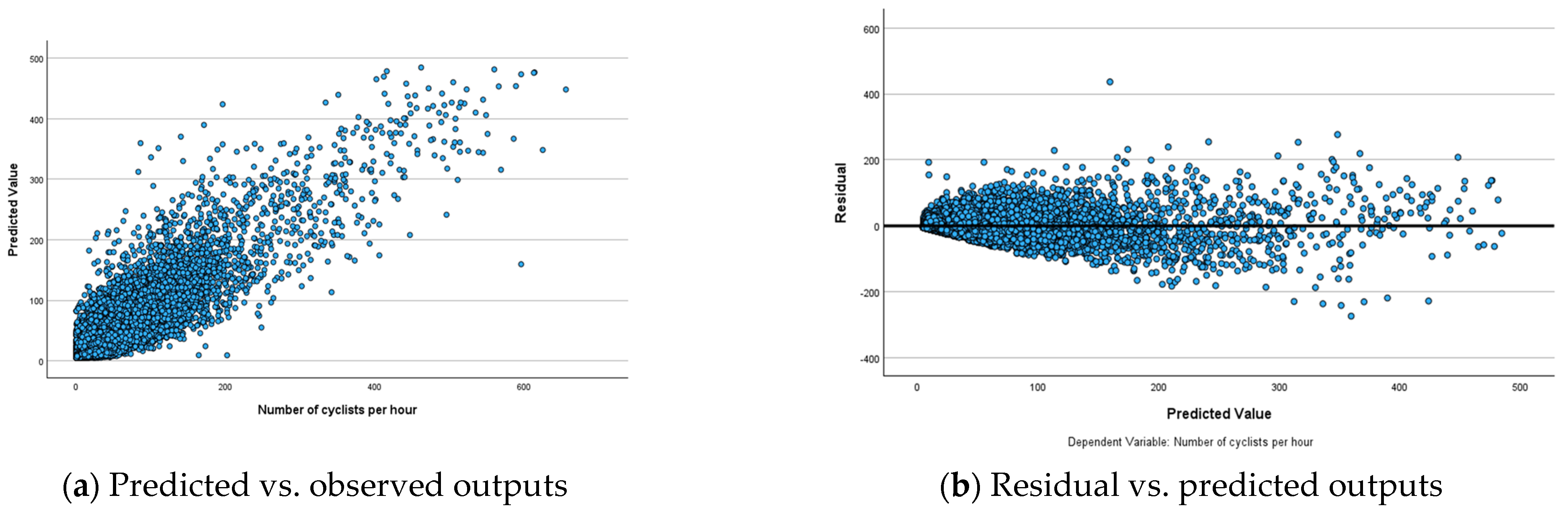
To analyse the performance of ANN models, predicted-by-observed and residual-by-observed scatterplots were generated (
Figure 3,
Figure 4 and
Figure 5). These visualisations help in understanding the relationships between predicted and observed values and residuals and observed values, respectively. In the predicted-by-observed scatterplots, the y-axis represents the predicted number of bicyclists, while the x-axis represents the observed number of bicyclists for the combined training and testing datasets before (
Figure 3a), during (
Figure 4a) and after (
Figure 5a) scenarios of the Mill Road Bridge closure. Ideally, the data points should align closely along a 45-degree line originating from the origin, indicating that the model’s predictions are accurate and unbiased. The scatterplots for before, during and after scenarios reveal that ANN models perform reasonably well in predicting the amount of bicycle traffic (
Figure 3a,
Figure 4a and
Figure 5a). The clustering of points along the 45-degree reference line suggests that ANN models successfully captured the underlying relationships within the datasets demonstrating strong predictive accuracy.
The residual-by-observed scatterplots were generated to analyse the distribution of residuals in relation to the predicted bicycle traffic (
Figure 3b,
Figure 4b and
Figure 5b). In these plots, the
y-axis represents the residuals, while the
x-axis represents the predicted values of bicycle traffic. This visualisation helps assess the overall fit and behaviour of the network’s predictions. The residual-by-predicted scatterplots for three scenarios exhibit a well-behaved and randomly scattered pattern, indicating a good model fit. ANN models effectively captured the underlying relationships for these scenarios without significant bias. The residuals formed a horizontal band and randomly fluctuated around the zero-line, indicating well-fitted models with few outliers (
Figure 3b,
Figure 4b and
Figure 5b). However, these outliers did not significantly affect the estimation of ANN models, ensuring the robustness of overall model performance.
4.2. Parameter Estimation of Input Variables
The predictive variables (input features) were initially fed into the input layer of ANN models. These inputs propagate to the hidden layers, which process the data and help extract complex patterns. This paper employed the Multi-Layer Perceptron (MLP) network to predict an output value by using a set of input variables. The MLP network is essentially a feedforward neural network to find out the optimal relationship between inputs and outputs by minimising the prediction errors. To achieve the best predictive accuracy, the MLP minimises the prediction error of its outputs. The MLP network was trained to optimise the weights such that the output predictions are as close as possible to the actual values. This involved adjusting the weights iteratively through an optimisation procedure. The MLP procedure computed the minimum and maximum values of a given range to help determine the appropriate number of hidden layers for minimising errors. Bayesian Information Criterion (BIC) was used to evaluate the model’s fitness and complexity. By minimising both the prediction error and BIC, the MLP aimed to find the most efficient model.
The best-performing configuration was two hidden layers for the ANN models for three scenarios, as two hidden layers achieved the optimal balance between complexity and predictive accuracy (
Table A1,
Table A2 and
Table A3). In the first hidden layer, the input data are distributed into three sub-layers, denoted as H(1:1), H(1:2) and H(1:3) (
Table A1,
Table A2 and
Table A3). These sub-layers represent different processing units that further refine the input data to capture various features or interactions in the datasets. Multiple sub-layers can enhance the network’s ability to model complex relationships. In addition, the sigmoid activation function was applied to the hidden layers. The sigmoid function transformed the input to the hidden layer into an output, and its Gaussian “bump” property helped smooth transition between inputs and output. The Gaussian “bump” refers to the shape of the curve that the sigmoid function created, helping the network capture underlying patterns in the data.
5. Discussion
The ANN models conducted sensitivity analyses to assess the importance of input variables in determining the spatial distribution of bicycle traffic based on the combined training and testing datasets (
Table 4,
Table 5 and
Table 6). The importance of an input variable is measured by how much the bicycle traffic changes as the value of a particular input variable changes. This allows the most influential factors for bicycle traffic to be identified. The spatial distribution of bicycle traffic was primarily determined by the hourly volume of motorbikes (44%), buses (34%) and sensors’ proximity to the Mill Road Bridge before the closure of the bridge (
Table 4). Interestingly, the spatial distribution of pedestrians is equally affected by the input variables of bicycle traffic for three scenarios (
Table 4,
Table 5 and
Table 6).
During the closure of the Mill Road Bridge, the most important variable was the sensors’ proximity to the Mill Road Bridge (99%), followed by number of large rigid vehicles (four axles and more) per hour (51%) (
Table 5). Bicyclists were forced to take alternative routes, resulting in longer travel times and less direct paths. If detour routes are not bike-friendly, such as roads with high commercial and large vehicles, lack of bicycle lanes and unsafe conditions, cyclists might face increasing safety risks and discomfort during their ride. In addition, the narrow and congested alternative routes could create conflict between bicycles and vehicles, potentially leading to accidents and delays.
The sensors’ proximity to the Mill Road Bridge was still contributing to the spatial distribution of bicycle traffic after the opening of the Mill Road Bridge (
Table 6). There might be insufficient or unclear signage indicating that the road is now open to traffic or directing cyclists and other road users to appropriate routes. Cyclists might still assume that the road was closed or dangerous, leading them to avoid the area or continue using detour routes even though the road is safe for cycling again. Moreover, the volumes of motorbikes (17%) and large vehicles with two and three axles (24%) significantly affected bicycle traffic after the opening of Mill Road Bridge (
Table 6). In general, cyclists face significant safety risks when riding in mixed traffic of motorcycles and large vehicles. These risks include limited visibility, speed discrepancies and unpredictable manoeuvres, especially with trucks and buses. Cyclists may also be affected by air turbulence from large vehicles and unsafe road conditions. To improve safety, dedicated bike lanes, reduced speed limits, cyclist and driver education, clear signage and stricter traffic law enforcement are essential. These measures can help reduce accidents and ensure a safer environment for cyclists in mixed traffic conditions.
6. Conclusions
The variability and big data size of sensor traffic data make it challenging to develop a single model capable of accurately analysing the nonrecurrent traffic distribution across the selected roads. Efficient methods are essential for analysing distribution patterns of motorised and non-motorised traffic in road networks near NRC events. The ANN can predict results with greater accuracy and determine the importance of explanatory variables without statistical errors in interpreting the traffic distribution. This paper builds on the demonstrated advantages of using ANN for traffic data analysis and integrates the GDR algorithm to analyse the sensor traffic data before, during and after the closure of the Mill Road Bridge.
The ANN models estimated that motorbike volume (44%), bus volume (34%) and proximity to the bridge were the most important factors influencing bicycle traffic distribution before the Mill Road Bridge closure. During the closure, proximity to the bridge (99%) and large rigid vehicle volume (51%) were the most significant factors forcing cyclists onto less safe detours. After reopening, proximity to the bridge still influenced traffic, possibly due to unclear signage. Motorbike (17%) and large vehicle (24%) volumes also impacted cyclists. This study highlights safety risks from mixed traffic and suggests dedicated bike lanes, speed limits, education, signage and stricter traffic laws to improve cyclist safety. Several studies suggested the cost-effectiveness of dedicated bike lanes across public safety, health, economic development and environmental impact. The New York State Department of Transportation [
43] observed that dedicated bike lanes reduced the injuries of all road users by up to 40%. Similarly, Kiani et al. [
44] observed that the expansion of cycling infrastructure, including dedicated bike lanes, was associated with increased cycling rates in Montreal, Canada. Macmillan et al. [
45] estimated that investing NZD 10 million in cycling infrastructure in New Zealand returned over NZD 24 million in healthcare savings due to increased physical activity that resulted in NZD 2.50 to NZD 5 returns in health and productivity benefits for every NZD 1 investment in bicycle infrastructure in New Zealand [
45]. Monsere et al. [
46] found that bicycle lanes could improve business with minimal negative impact on sales and employment in five cities of the United States of America, such as Austin (Texas); Chicago (Illinois); Portland (Oregon); San Francisco (California); and Washington (District Columbia).
The findings highlight the importance of accurate traffic congestion detection for traveller information systems and traffic control. This paper focuses on congestion clusters, emphasising a cost-effective approach using sensors to monitor key locations rather than the entire road network. By leveraging neural networks, the research aims to enhance traffic monitoring and forecasting, providing insights into traffic flow changes due to infrastructure modifications. However, several factors affect how traffic redistributes when a road closure occurs. The structure of the road network determines how easily traffic can reroute. A grid-like system offers more alternative paths than a network with limited connections. If multiple roads can absorb diverted traffic, congestion may be less severe. If options are limited, bottlenecks are more likely. Traffic lights can be adjusted to improve flow on detour routes, reducing congestion in affected areas. Tools like variable message signs, smart traffic signals and ramp metering can help regulate traffic flow and minimise delays. Notably, sensors such as inductive loop detectors, radar, cameras and Bluetooth trackers enable data-driven decision-making systems for dynamic traffic redistribution. These systems analyse traffic conditions such as vehicle speed, density and queue length and automatically adjust traffic light timings, update variable message signs and integrate with navigation systems to reroute traffic. The continuous flow of sensor data enables rapid responses to congestion, ensuring minimal delays and improving the safety of both road users and workers. This adaptive approach results in more efficient traffic management and safer work zone environments. However, the loss of data, inaccurate traffic reporting and increased traffic congestion may result from hardware and power failures, signal interference, software and calibration errors and environmental obstructions to traffic sensors. It is important to carefully plan and place sensors and supplement and combine data from vehicles, drones and smartphone devices. The traffic management systems of local councils can use a combination of data filtering, sensor fusion, redundancy and advanced analytical tools to ensure robustness and actionable traffic data. Regular sensor maintenance, along with real-time monitoring, can further reduce the impact of these challenges.
Future studies should focus on including these challenges within ANN models predicting the spatial distribution of bicycle traffic before, during and after the closure of a road or transport sub-system. Cities that plan proactively for bicycle traffic during road closures can minimise disruptions by temporarily adjusting infrastructure to accommodate cyclists. This might include installing bike lanes, rerouting paths and creating temporary bike-sharing stations. Additionally, wayfinding measures, such as clear signage and digital apps, can guide cyclists safely around the closure areas. These efforts help ensure that cycling remains a convenient, safe and sustainable mode of transport even when regular routes are interrupted.


