
Fault Diagnosis of Bearings with Small Sample Size Using Improved Capsule Network and Siamese Neural Network

Abstract
1. Introduction
2. Related Work
2.1. Few-Shot Learning
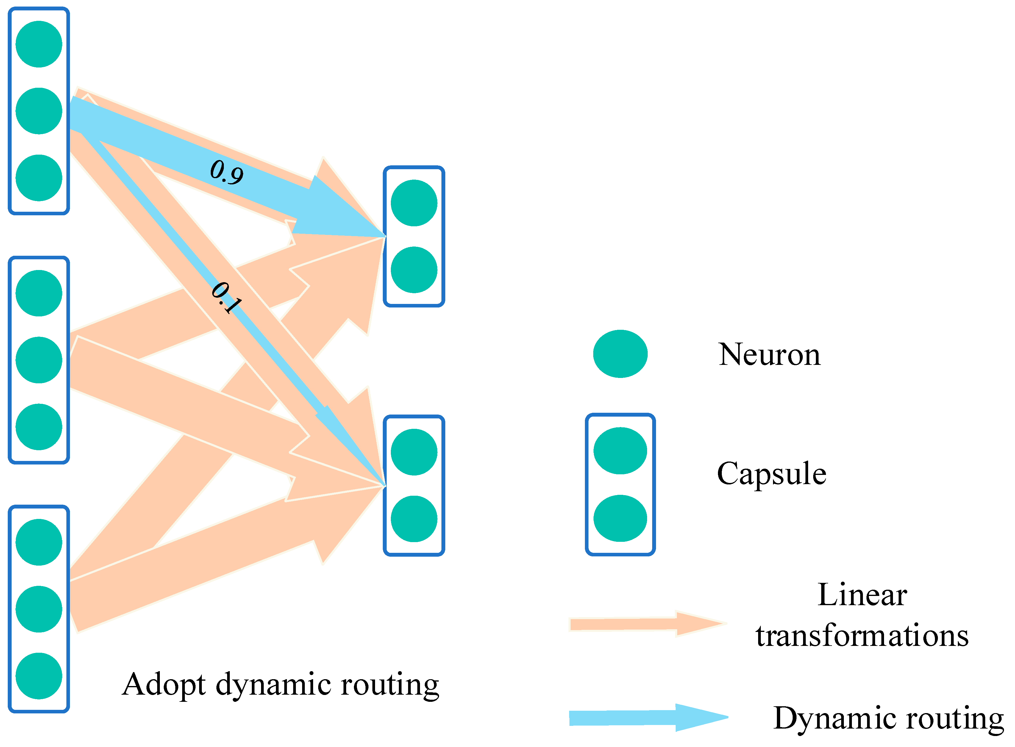
2.2. Capsule Network
2.3. Siamese Network
Introduction to Distance Metric Functions
3. Proposed Method
3.1. Multi-View Joint Optimization for Feature Extraction
- (1)
- Window Size 1024, Stride 40: This segmentation method generates images that are relatively dense along the time axis and have a moderate time span. Each image contains 1024 consecutive data points, with an overlap of 98.4% (i.e., (1024−40)/1024) between adjacent images, helping the model capture subtle changes in the signal;
- (2)
- Window Size 1024, Stride 80: Compared to the first method, this generates images that are less dense along the time axis but contain more temporal information. The overlap between adjacent images decreases to 92.2%, aiding the model in understanding the overall trend of the signal from a broader perspective;
- (3)
- Window Size 2048, Stride 40: By increasing the window size to 2048, this method generates images with a larger time span. Maintaining a stride of 40 ensures a high temporal density, allowing the model to capture both local and global features of the signal simultaneously;
- (4)
- Window Size 2048, Stride 80: This is the segmentation method with the largest time span and the lowest temporal density. Each image contains 2048 data points, with an overlap of 96.1% between adjacent images.
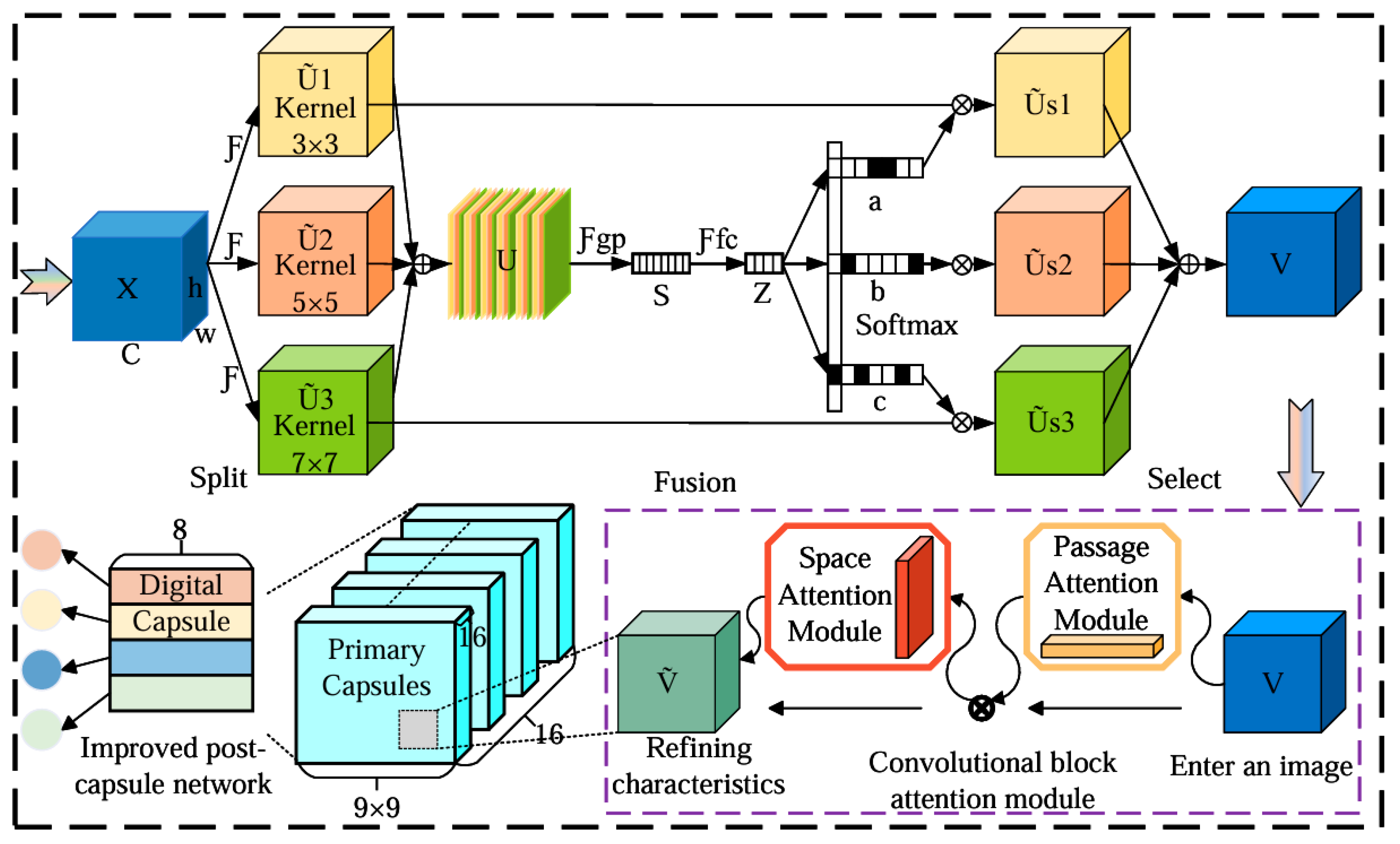
3.2. Improved Capsule Network Architecture
3.2.1. Internal Structure of Capsule Network
3.2.2. Capsule Network Parameters
3.2.3. Output Shape and Parameter Calculation of the Siamese Capsule Network
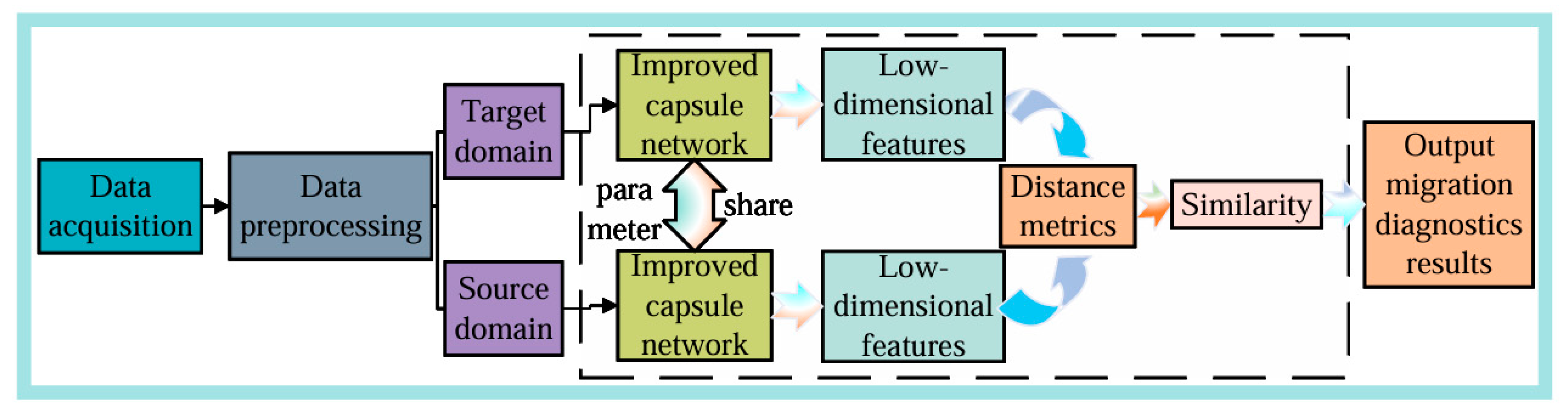
3.3. Transfer Network Construction and Workflow
- (1)
- Source Domain Data Preparation: Traditional rolling bearing vibration signals serve as the source domain data. Following the preprocessing steps outlined in Section 3.1, the corresponding source domain dataset is constructed;
- (2)
- Model Training on Source Domain: The fault diagnosis model based on the Siamese capsule network is trained using the constructed source domain dataset. The Siamese capsule network comprises two identical branches with shared weights, enabling it to learn the spatial hierarchical structure and dynamic routing relationships between features. Ensure that the model is fully trained to obtain a well-performing source domain fault diagnosis model;
- (3)
- Target Domain Data Preparation: Another portion of the rolling bearing vibration signals is selected as target domain data. Following the same preprocessing steps outlined in Section 3.1, the corresponding target domain dataset is constructed;
- (4)
- Parameter Transfer: The architecture and weight parameters of the capsule network branches from the source domain fault diagnosis model are transferred to the target domain diagnosis model. According to the predefined parameter update strategy, certain transferred parameters (typically the capsule layers responsible for extracting low-level features) are retained and frozen to ensure they do not participate in subsequent training. This step ensures the transfer and retention of knowledge;
- (5)
- Fine-Tuning on Target Domain: Using the target domain training dataset, the target domain diagnosis model is trained based on the frozen parameters. The remaining network parameters and weights are fine-tuned. The goal of fine-tuning is to enable the newly added capsule layers to adapt to the data distribution of the target domain and optimize the performance of the Siamese capsule network on the target domain;
- (6)
- Model Testing: After training the target domain diagnosis model, it is tested using the test dataset. The diagnostic accuracy of the model for bearing faults is evaluated by computing the similarity or distance between test sample pairs. The final diagnostic accuracy is used to measure the model’s performance.
4. Experimental Verification
4.1. Data Augmentation
4.2. CWRU Bearing Dataset
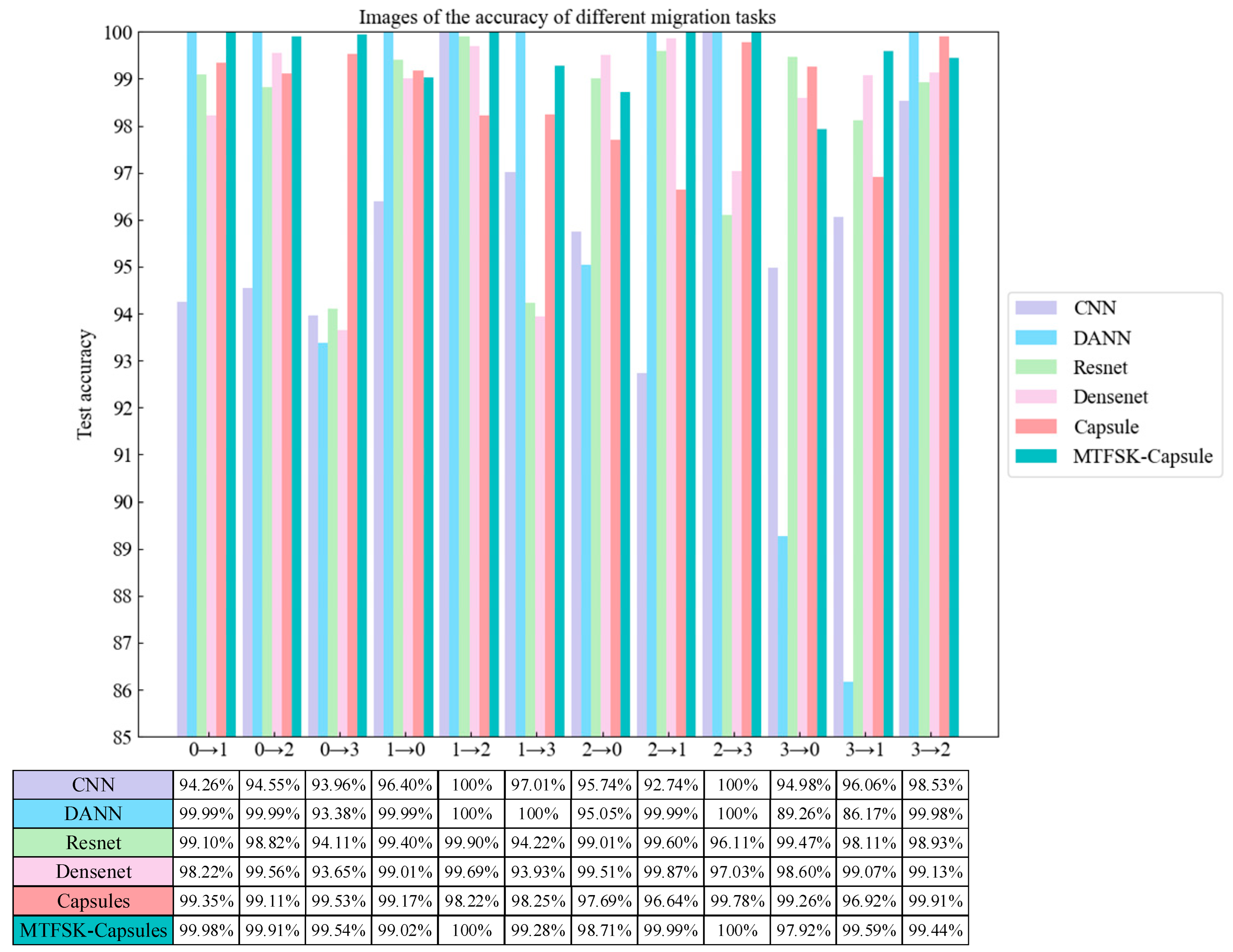
4.2.1. Comparative Ablation Study (CWRU Dataset)
4.2.2. Noise Resistance Experiment (CWRU Dataset)
4.2.3. Dimensionality Reduction Visualization (CWRU Dataset)
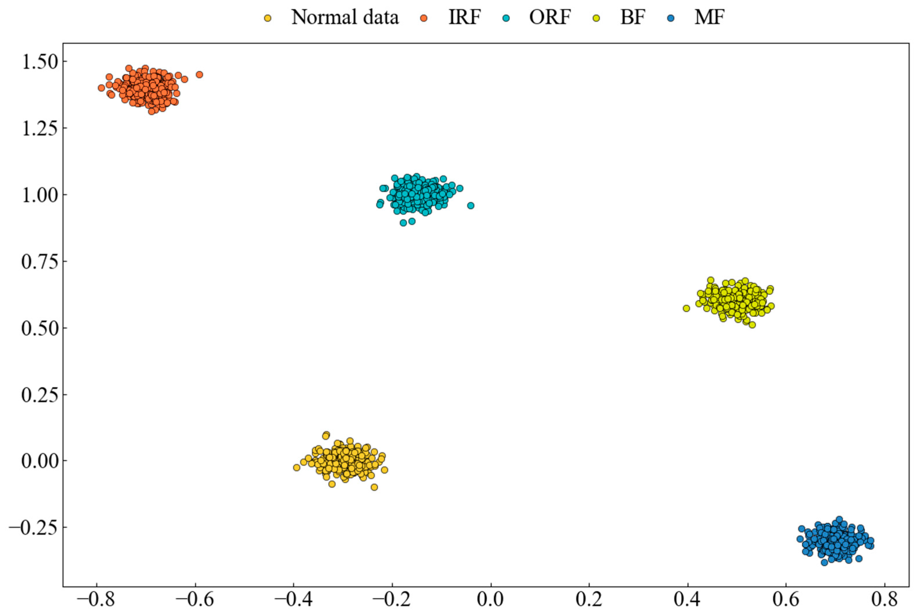
- (1)
- Class Boundary Identification: t-SNE visualization allows for the observation of distinct separations between different data classes, providing insights into how the network learns and distinguishes class information;
- (2)
- Clustering Structure in Feature Space: t-SNE highlights the clustering of similar samples within the feature space, helping to understand the feature representation in the intermediate layers and the network’s classification process.
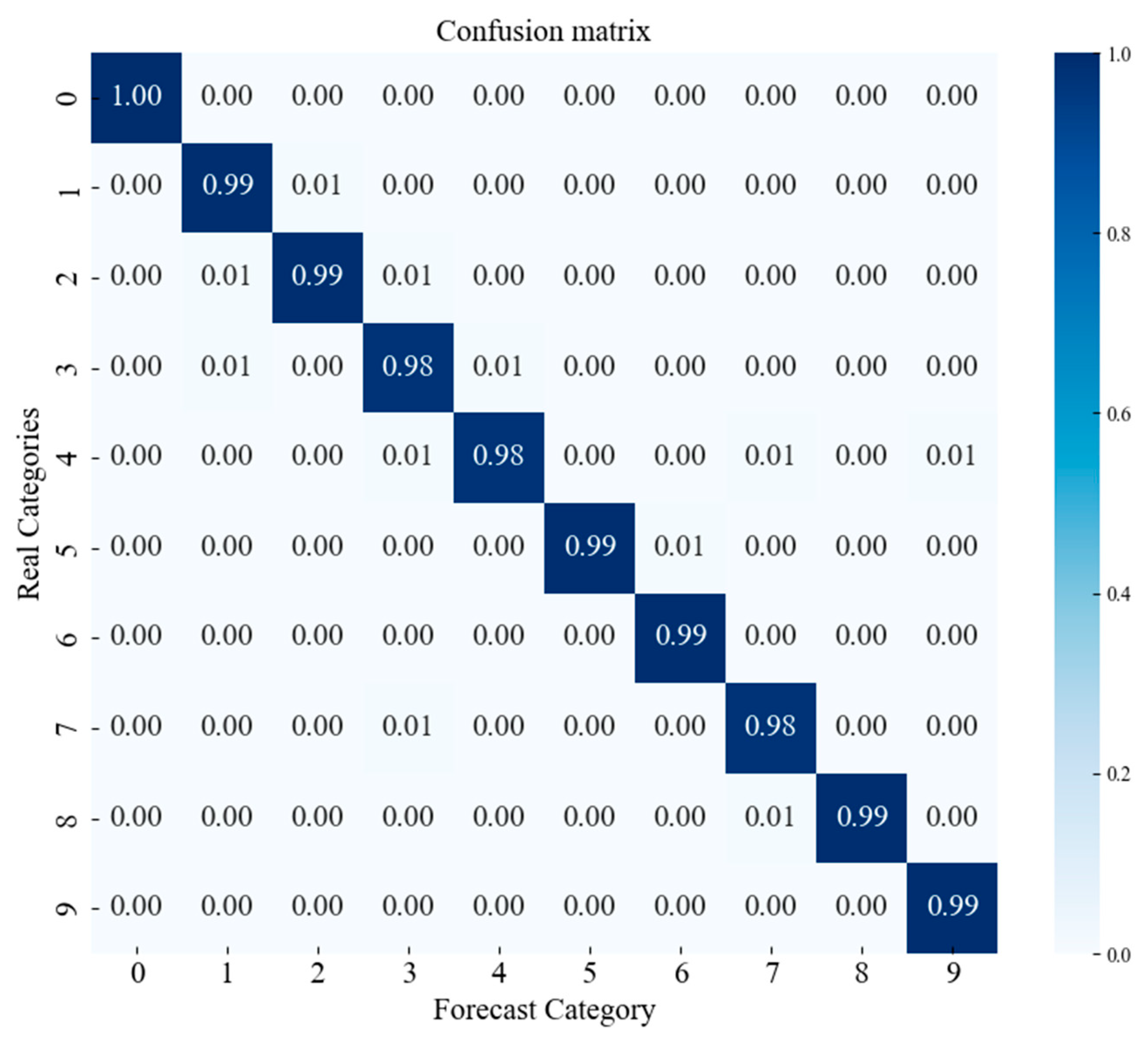
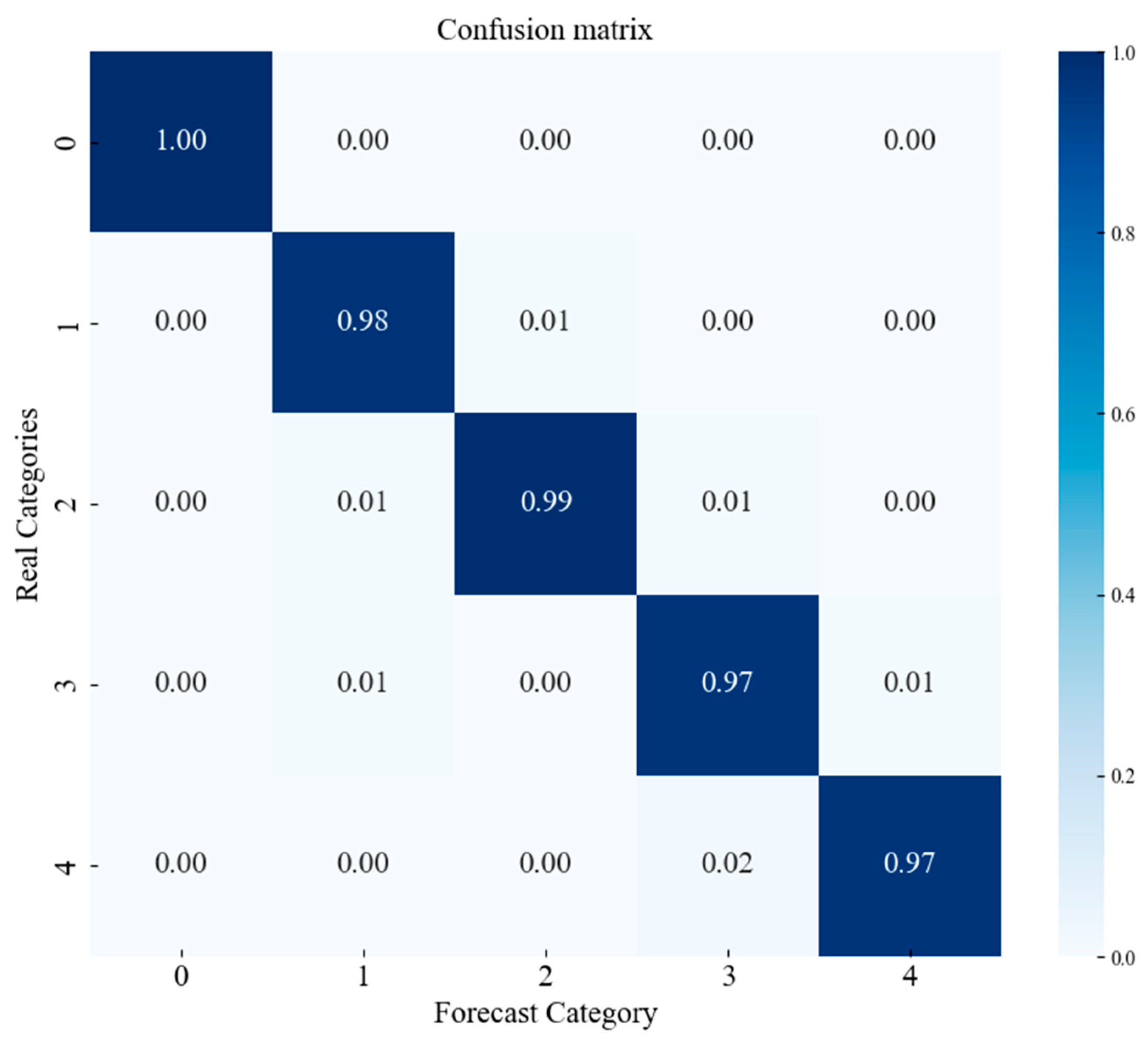
4.2.4. Confusion Matrix (CWRU Dataset)
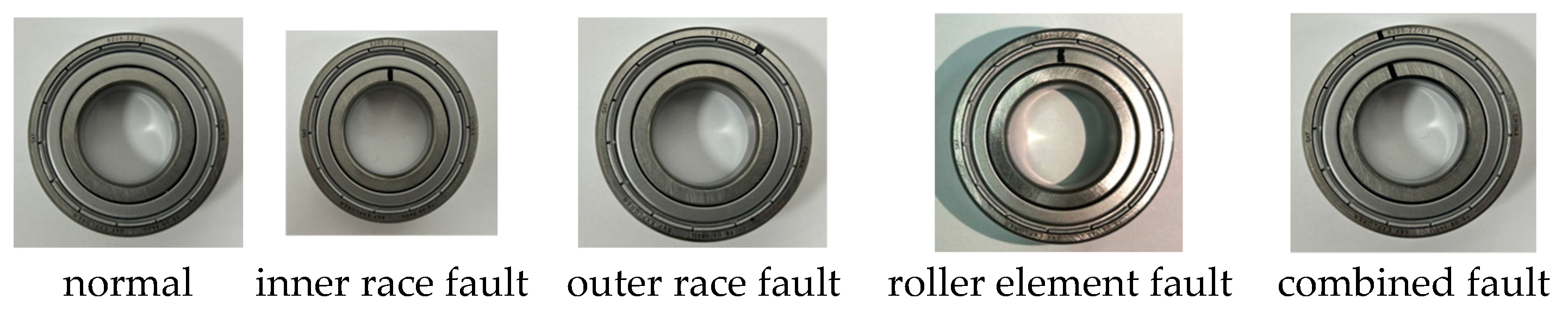
4.3. Laboratory Bearing Dataset
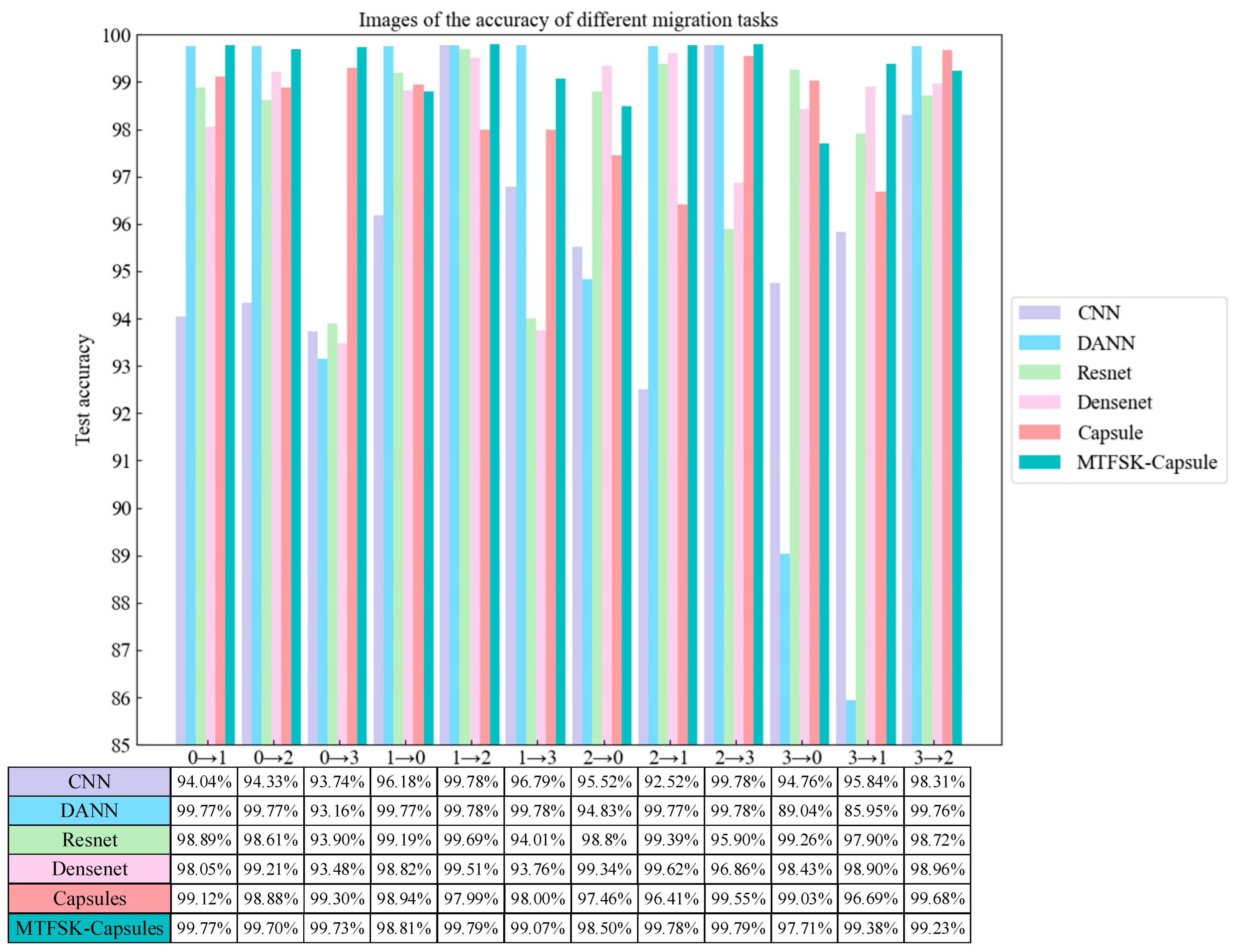
4.3.1. Comparative Ablation Study (Laboratory Bearing Dataset)
4.3.2. Noise Resistance Experiment (Laboratory Bearing Dataset)
4.3.3. Dimensionality Reduction Visualization (Laboratory Bearing Dataset)
4.3.4. Confusion Matrix (Laboratory Bearing Dataset)
5. Conclusions
Author Contributions
Funding
Institutional Review Board Statement
Informed Consent Statement
Data Availability Statement
Conflicts of Interest
Appendix A
| import torch.nn as nn import torch from .baseModels import PrimaryCaps, DigitCaps from cbam import cbam_block from SKNet import SKConv import torch.nn.functional as F device = “cuda” if torch.cuda.is_available() else “cpu” class CapsNet(nn.Module): ‘‘‘ Basic implementation of capsule network layer ‘‘‘ def __init__(self, img_w, img_h, num_classes): super(CapsNet, self).__init__() self.num_classes = num_classes # Conv2d layer self.conv1 = nn.Conv2d(1, 64, 3, 1) self.relu = nn.ReLU(inplace = False) # self.cbam = cbam_block(64) self.sknet = SKConv(64, M = 3, G = 1, r = 3, outFeatures = 64) # Primary capsule self.primary_caps = PrimaryCaps(num_conv_units = 16, in_channels = 64, out_channels = 16, kernel_size = 9, stride = 2) self.layerNorm = nn.LayerNorm # Digit capsule self.digit_caps = DigitCaps(in_dim = 16, in_caps = 1296, out_caps = num_classes, out_dim = 8, num_routing = 16) self.digit_caps.setDevice(device) # Reconstruction layer self.decoder = nn.Sequential( nn.Linear(num_classes * 8, 128), nn.ReLU(inplace = True), nn.Linear(128, 256), nn.ReLU(inplace = True), nn.Linear(256, img_w*img_h), # nn.Sigmoid() ) def forward(self, x): out1 = self.conv1(x) # print(0, out1.shape) out2 = self.relu(out1) out3 = self.sknet(out2) # print(1, out3.shape) out4 = self.relu(out3) # out = F.dropout(out, 0.5) out5 = self.primary_caps(out4) # print(2, out5.shape) out6 = self.digit_caps(out5) # print(3, out6.shape) # Shape of logits: [batch_size, out_capsules] logits = torch.norm(out6, dim=–1) pred = torch.eye(self.num_classes).to(device).index_select(dim = 0, index = torch.argmax(logits, dim = 1)) # Reconstruction batch_size = out6.shape[0] reconstruction = self.decoder((out6 * pred.unsqueeze(2)).contiguous().view(batch_size, –1)) return logits, reconstruction from torch import nn import torch class Exping(nn.Module): def __init__(self): super(Exping, self).__init__() def forward(self, x): return torch.exp(x) * torch.sin(x) # Apply Exping to the corresponding layers in the neural network. model = nn.Sequential( nn.Linear(10, 20), Exping(), nn.Linear(20, 1) ) class SKConv(nn.Module): def __init__(self, features, M, G, r, stride = 1, L = 16, outFeatures = 128): super(SKConv, self).__init__() d = max(int(features / r), L) self.M = int(M) self.features = features self.outFeatures = outFeatures self.convs = nn.ModuleList([]) for i in range(self.M): # Convolutions with different kernel sizes self.convs.append( nn.Sequential( nn.Conv2d(features, self.outFeatures, # kernel_size = 3 + i * 2, kernel_size = (1, 3 + i * 2), stride = stride, padding = (0, i+1), groups = G), nn.BatchNorm2d(self.outFeatures), nn.ReLU(inplace = False))) self.fc = nn.Linear(self.outFeatures, d) self.fcs = nn.ModuleList([]) for i in range(self.M): self.fcs.append(nn.Linear(d, outFeatures)) self.softmax = nn.Softmax(dim = 1) def forward(self, x): for i, conv in enumerate(self.convs): fea = conv(x).unsqueeze(dim = 1) if i == 0: feas = fea else: feas = torch.cat([feas, fea], dim = 1) fea_U = torch.sum(feas, dim = 1) fea_s = fea_U.mean(–1).mean(–1) fea_z = self.fc(fea_s) for i, fc in enumerate(self.fcs): # print(i, fea_z.shape) vector = fc(fea_z).unsqueeze(dim = 1) # print(i, vector.shape) if i == 0: attention_vectors = vector else: attention_vectors = torch.cat([attention_vectors, vector], dim = 1) attention_vectors = self.softmax(attention_vectors) attention_vectors = attention_vectors.unsqueeze(–1).unsqueeze(–1) fea_v = (feas * attention_vectors).sum(dim = 1) return fea_v |
References
- Tang, J. Research on Rolling Bearing Fault Diagnosis Based on Object Detection Theory. Ph.D. Thesis, Xi’an University of Technology, Xi’an, China, 2023. [Google Scholar]
- Liu, Y. Research on Fault Diagnosis Methods for Rotating Machinery Under Variable Speed Conditions. Ph.D. Thesis, Guilin University of Electronic Technology, Guilin, China, 2023. [Google Scholar]
- Zhou, X.; Li, A.; Han, G. An Intelligent Multi-Local Model Bearing Fault Diagnosis Method Using Small Sample Fusion. Sensors 2023, 23, 7567. [Google Scholar] [CrossRef]
- Yang, G.; Xu, W.-Y.; Deng, Q.; Wei, Y.-Q.; Li, F. Review of Composite Fault Diagnosis of Rolling Bearings Based on Vibration Signals. J. Xihua Univ. (Nat. Sci. Ed.) 2024, 43, 48–69. [Google Scholar]
- Yan, P.; Abdulkadir, A.; Luley, P.P.; Rosenthal, M.; Schatte, G.A.; Grewe, B.F.; Stadelmann, T. A Comprehensive Survey of Deep Transfer Learning for Anomaly Detection in Industrial Time Series: Methods, Applications, and Directions. IEEE Access 2024, 12, 3768–3789. [Google Scholar] [CrossRef]
- Liu, C.-Y.; Li, Z.-N.; Xiong, P.-W. Research on Fault Diagnosis Method Based on Swin Transformer with Path Aggregation Network. J. Vib. Shock 2024, 43, 258–266. [Google Scholar]
- Kang, Y.-X.; Chen, G.; Wei, X.-K.; Pan, W.-P.; Wang, H. Multi-Task Diagnosis Method for Rolling Bearings in Aero-Engines Based on Residual Network. J. Vib. Shock 2022, 41, 285–293. [Google Scholar]
- Zhang, R.-C.; Sun, W.-L.; Liang, W.-Z. Research on Fault Diagnosis of Industrial Processes Based on SSAE-IARO-BiLSTM. J. Vib. Shock 2024, 43, 244–250+260. [Google Scholar]
- Zhang, B.-W.; Pang, X.-Y.; Cheng, B.-A.; Li, F.; Suo, S.-Z. Research on Fault Diagnosis Method for Aero-Engine Bearings Based on PIRD-CNN. J. Vib. Shock 2024, 43, 201–207+231. [Google Scholar]
- Lei, C.-L.; Xia, B.-F.; Xue, L.-L.; Jiao, M.-X.; Zhang, H.-Q. Fault Diagnosis Method for Rolling Bearings Based on MTF-CNN. J. Vib. Shock 2022, 41, 151–158. [Google Scholar]
- Guan, Y.-L.; Liu, G.-L.; Yu, C.-Y.; Yang, X.-X.; Jing, L.-Y. Fault Diagnosis Method for Rolling Bearings Based on CNN and BLS. J. Vib. Test. Diagn. 2024, 44, 1017–1022+1044. [Google Scholar]
- Wu, N.; Wang, J.; Yang, J.-W.; Lv, B. Review of Transfer Learning Methods for Rolling Bearing Fault Diagnosis under Variable Working Conditions and Small Sample Sizes. Sci. Technol. Eng. 2024, 24, 3939–3951. [Google Scholar]
- Zhao, X.-P.; Peng, P.; Zhang, Y.-H.; Zhang, Z.-Y. Application of Improved Siamese Network in Small Sample Bearing Fault Diagnosis. Comput. Eng. Appl. 2023, 59, 294–304. [Google Scholar]
- Wang, Z.-M.; Nie, X.-Y.; Wang, Y.-J.; Ji, C.-Q.; Qin, J. Fault Diagnosis Method for Bearings Based on Capsule Network under Small Sample Conditions. Comput. Eng. Des. 2023, 44, 1259–1266. [Google Scholar]
- Yuan, H.-F.; Zhang, X.-N.; Wang, H.-Q. Research on Composite Fault Diagnosis of Bearings Based on Improved Capsule Network. J. Vib. Shock 2023, 42, 69–76+123. [Google Scholar]
- Zhang, T.; Chen, J.; Li, F.; Zhang, K.; Lv, H.; He, S.; Xu, E. Intelligent Fault Diagnosis of Machines with Small & Imbalanced Data: A State-of-the-Art Review and Possible Extensions. ISA Trans. 2022, 119, 152–171. [Google Scholar] [PubMed]
- Hu, M.-W. Research on Fault Diagnosis Methods for Rolling Bearings Under Variable Working Conditions Based on Transfer Learning. Ph.D. Thesis, Harbin University of Science and Technology, Harbin, China, 2019. [Google Scholar]
- Lu, W.; Liu, J.; Lin, F. Fault Diagnosis of Rolling Bearings Using a Dual-Branch Convolutional Capsule Neural Network. Sensors 2024, 24, 3384. [Google Scholar] [CrossRef]
- Fu, P.; Wang, J.; Zhang, X.; Zhang, L.; Gao, R.X. Dynamic Routing-Based Multimodal Neural Network for Multi-Sensory Fault Diagnosis of Induction Motor. J. Manuf. Syst. 2020, 55, 264–272. [Google Scholar] [CrossRef]
- Zhao, Z.-H.; Zhang, R.; Liu, K.-J.; Yang, S.-P. A Small Sample Bearing Fault Diagnosis Method Based on Improved Prototypical Network. J. Vib. Shock 2023, 42, 214–221. [Google Scholar]
- Hao, W.; Ding, K.; Bao, C.-C.; He, T.-T.; Chen, Y.-H.; Zhang, K. Bearing Fault Diagnosis Method Based on Multi-Scale Convolutional Relational Network under Small Sample Conditions. China Test 2024, 50, 160–168. [Google Scholar]
- Yang, X.-H.; Zhang, L.; Ye, L. Small Sample Knowledge Graph Completion Based on Adaptive Context Matching Network. Comput. Sci. 2024, 51, 223–231. [Google Scholar]
- Zhao, Z.-H.; Wu, D.-D. Research on Bearing Fault Diagnosis Based on Siamese Network Structure. Mach. Hydraul. 2023, 51, 202–208. [Google Scholar]
- Zhang, D.; Ren, X.; Zuo, H. Compound Fault Diagnosis for Gearbox Based Using of Euclidean Matrix Sample Entropy and One-Dimensional Convolutional Neural Network. Shock Vib. 2021, 2021, 6669006. [Google Scholar] [CrossRef]
- He, C.; Yasenjiang, J.; Lv, L.; Xu, L.; Lan, Z. Gearbox Fault Diagnosis Based on MSCNN-LSTMCBAM-SE. Sensors 2024, 24, 4682. [Google Scholar] [CrossRef]
- Wang, H.; Liu, Z.; Li, M.; Dai, X.; Wang, R.; Shi, L. A Gearbox Fault Diagnosis Method Based on Graph Neural Networks and Markov Transform Fields. IEEE Sens. J. 2024, 24, 25186–25196. [Google Scholar] [CrossRef]
- Smith, W.A.; Randall, R.B. Rolling element bearing diagnostics using the Case Western Reserve University data: A benchmark study. Mech. Syst. Signal Process. 2015, 64–65, 100–131. [Google Scholar] [CrossRef]


| Step | Operation | Formula/Detailed Description |
|---|---|---|
| 1 | Determine Input Vectors | Assume there are two n-dimensional vectors, X and Y, represented as X = (x1, x2, …, xn) and Y = (y1, y2, …, yn). |
| 2 | Calculate Differences in Each Dimension | For each dimension i (i = 1, 2, …, n), calculate the difference between the vectors X and Y in that dimension, i.e., di = xi−yi. This will generate a difference vector D = (d1, d2, …, dn). |
| 3 | Compute Squares of the Differences | For each element di (i = 1, 2, …, n) in the difference vector D, compute its square value, i.e., di2 = (xi − yi)2. This will generate a squared difference vector D2 = (d12, d22, …, dn2). |
| 4 | Calculate the Sum of Squares | Sum all the elements in the squared difference vector D2 to obtain the sum of squares S, i.e., S = ∑(di2) = d12 + d22 + … + dn2. This is the total sum of the squares of the differences between the two vectors. |
| 5 | Compute Euclidean Distance | Take the square root of the sum of squares S to obtain the Euclidean distance d, i.e., |
| Layer | Network Parameters | |
|---|---|---|
| MTF | ||
| Conv (SKNet) | (64,64), K = 3, S = 1, P = 1 | SKNet Channel 1 |
| (64,64), K = 5, S = 1, P = 2 | SKNet Channel 2 | |
| (64,64), K = 7, S = 1, P = 3 | SKNet Channel 3 | |
| Primary capsule | Num_conv_units = 16 | Primary capsule |
| In_channels = 64 | Input | |
| Out_channels = 16 | Output Channels | |
| Kernel_size = 9 | Kernel Size | |
| Stride = 2 | Stride | |
| Digit_caps | In_dim = 16 | Input Capsule Dimension |
| In_caps = 1296 | Input Capsule Number | |
| Out_caps = 4 | Output Capsule Number | |
| Out_dim = 8 | Output Capsule Vector Dimension | |
| Num_routing = 16 | Routing Algorithm Iterations |
| Module | Output Shape | Computational Parameters |
|---|---|---|
| Conv2d | (64, 26, 26) | 2368 |
| ReLU | (64, 26, 26) | 0 |
| SKConv | (64, 26, 26) | 77,056 |
| PrimaryCaps | (16, 6, 6) | 200,704 |
| Reconstruction (decoder) | (28 × 28) | 136,960 |
| Reshape | (28, 28) | 0 |
| Flatten | (784) | 0 |
| Fully Connected | (num_classes) | 0 |
| Softmax | (num_classes) | 0 |
| Label | Bearing Condition | Damage Location | Rotation Speed | Damage Length |
|---|---|---|---|---|
| 0 | Normal | Normal | 1797 rpm | 0 |
| 1 | Fault | Inner Race | 1797 rpm | 0.007 |
| 2 | Fault | Inner Race | 1797 rpm | 0.014 |
| 3 | Fault | Inner Race | 1797 rpm | 0.021 |
| 4 | Fault | Outer Race | 1797 rpm | 0.007 |
| 5 | Fault | Outer Race | 1797 rpm | 0.014 |
| 6 | Fault | Outer Race | 1797 rpm | 0.021 |
| 7 | Fault | Roller Element | 1797 rpm | 0.007 |
| 8 | Fault | Roller Element | 1797 rpm | 0.014 |
| 9 | Fault | Roller Element | 1797 rpm | 0.021 |
| Dataset | Category | Sample Count | Fault Location |
|---|---|---|---|
| A | training set | 800 | normal |
| test set | 200 | ||
| B | training set | 100 | inner race |
| test set | 900 | ||
| C | training set | 100 | outer race |
| test set | 900 | ||
| D | training set | 100 | roller element |
| test set | 900 | ||
| E | training set | 100 | combined fault |
| test set | 900 |
Disclaimer/Publisher’s Note: The statements, opinions and data contained in all publications are solely those of the individual author(s) and contributor(s) and not of MDPI and/or the editor(s). MDPI and/or the editor(s) disclaim responsibility for any injury to people or property resulting from any ideas, methods, instructions or products referred to in the content. |
© 2024 by the authors. Licensee MDPI, Basel, Switzerland. This article is an open access article distributed under the terms and conditions of the Creative Commons Attribution (CC BY) license (https://creativecommons.org/licenses/by/4.0/).
Share and Cite
Yasenjiang, J.; Xiao, Y.; He, C.; Lv, L.; Wang, W. Fault Diagnosis of Bearings with Small Sample Size Using Improved Capsule Network and Siamese Neural Network. Sensors 2025, 25, 92. https://doi.org/10.3390/s25010092
Yasenjiang J, Xiao Y, He C, Lv L, Wang W. Fault Diagnosis of Bearings with Small Sample Size Using Improved Capsule Network and Siamese Neural Network. Sensors. 2025; 25(1):92. https://doi.org/10.3390/s25010092
Chicago/Turabian StyleYasenjiang, Jarula, Yang Xiao, Chao He, Luhui Lv, and Wenhao Wang. 2025. "Fault Diagnosis of Bearings with Small Sample Size Using Improved Capsule Network and Siamese Neural Network" Sensors 25, no. 1: 92. https://doi.org/10.3390/s25010092
APA StyleYasenjiang, J., Xiao, Y., He, C., Lv, L., & Wang, W. (2025). Fault Diagnosis of Bearings with Small Sample Size Using Improved Capsule Network and Siamese Neural Network. Sensors, 25(1), 92. https://doi.org/10.3390/s25010092