
Enhanced Sensor Placement Optimization and Defect Detection in Structural Health Monitoring Using Hybrid PI-DEIM Approach

 , ,
, ,  ,
, 
Abstract
1. Introduction
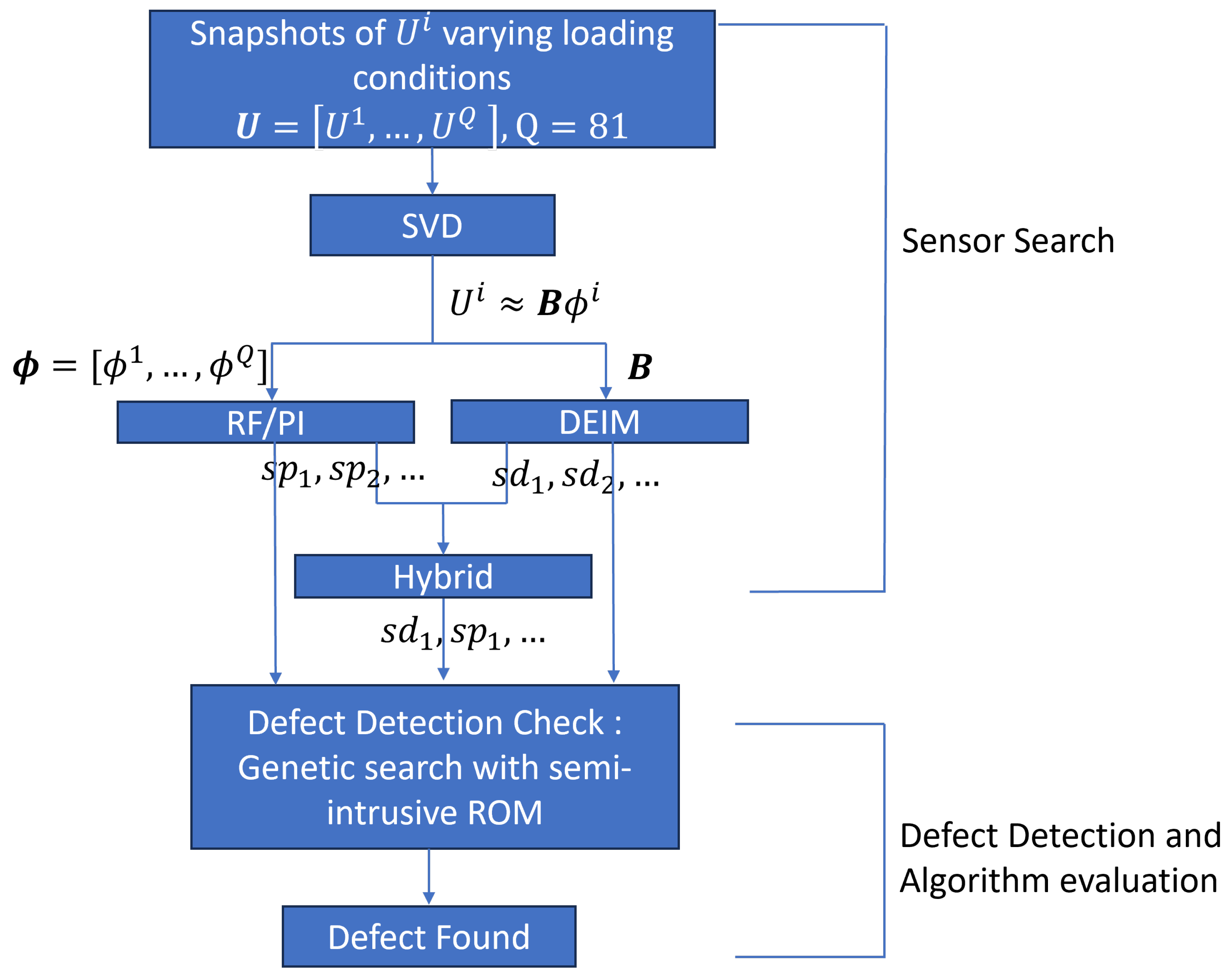
2. Method
2.1. Sensor Search
2.1.1. Constructing the Data Set and the Reduced Basis
2.1.2. Permutation Features Importance Method (PI)
2.1.3. Discrete Empirical Interpolation Method (DEIM)
2.1.4. Hybrid Method
2.2. Defect Detection
2.2.1. Lightly Intrusive ROM
2.2.2. Genetic Search Algorithm
2.2.3. Sensor Confirmation
3. Results and Discussion
3.1. Sensor Search
3.1.1. Permutation Features Importance Method (PI)
3.1.2. Discrete Empirical Interpolation Method (DEIM)
3.1.3. Hybrid
3.2. Defect Detection
3.2.1. Sensor Confirmation
3.2.2. Defect Detection
4. Conclusions
Author Contributions
Funding
Institutional Review Board Statement
Informed Consent Statement
Data Availability Statement
Acknowledgments
Conflicts of Interest
Appendix A

| Case | (m) | (m) | (m) | E (GPa) |
|---|---|---|---|---|
| 1 | 113 | |||
| 2 | 200 | |||
| 3 | 286 | |||
| 4 | 113 | |||
| 5 | 200 | |||
| 6 | 113 | |||
| 7 | 286 | |||
| 8 | 113 | |||
| 9 | 200 | |||
| 10 | 113 | |||
| 11 | 200 | |||
| 12 | 113 | |||
| 13 | 286 | |||
| 14 | 113 | |||
| 15 | 286 | |||
| 16 | 113 | |||
| 17 | 200 | |||
| 18 | 113 | |||
| 19 | 200 | |||
| 20 | 113 | |||
| 21 | 200 | |||
| 22 | 113 | |||
| 23 | 200 | |||
| 24 | 286 | |||
| 25 | 200 | |||
| 26 | 286 | |||
| 27 | 200 | |||
| 28 | 286 | |||
| 29 | 200 | |||
| 30 | 286 | |||
| 31 | 113 | |||
| 32 | 286 | |||
| 33 | 113 | |||
| 34 | 286 | |||
| 35 | 200 | |||
| 36 | 286 | |||
| 37 | 200 | |||
| 38 | 286 | |||
| 39 | 113 | |||
| 40 | 286 | |||
| 41 | 200 | |||
| 42 | 286 | |||
| 43 | 113 | |||
| 44 | 200 | |||
| 45 | 286 |
References
- Rodriguez, S.; Lorenzo, D.D.; Chinesta, F.; Monteiro, E.; Rebillat, M.; Mechbal, N. Hybrid Twin applied to Structural Health Monitoring. In Proceedings of the 10th ECCOMAS Thematic Conference on Smart Structures and Materials (SMART 2023), Patras, Greece, 3–5 July 2023; ECCOMAS: Barcelona, Spain, 2023; pp. 1851–1862. [Google Scholar] [CrossRef]
- Lorenzo, D.D.; Champaney, V.; Germoso, C.; Cueto, E.; Chinesta, F. Data Completion, Model Correction and Enrichment Based on Sparse Identification and Data Assimilation. Appl. Sci. 2022, 12, 7458. [Google Scholar] [CrossRef]
- Jiang, Y.; Li, D.; Song, G. On the physical significance of the Effective Independence method for sensor placement. J. Phys. Conf. Ser. 2017, 842, 012030. [Google Scholar] [CrossRef]
- Liu, J.; Hei, C.; Luo, M.; Yang, D.; Sun, C.; Feng, A. A Study on Impact Force Detection Method Based on Piezoelectric Sensing. Sensors 2022, 22, 5167. [Google Scholar] [CrossRef] [PubMed]
- Chen, B.; Hei, C.; Luo, M.; Ho, M.S.; Song, G. Pipeline two-dimensional impact location determination using time of arrival with instant phase (TOAIP) with piezoceramic transducer array. Smart Mater. Struct. 2018, 27, 105003. [Google Scholar] [CrossRef]
- Cheng, H.; Wang, F.; Huo, L.; Song, G. Detection of sand deposition in pipeline using percussion, voice recognition, and support vector machine. Struct. Health Monit. 2020, 19, 2075–2090. [Google Scholar] [CrossRef]
- Manohar, K.; Brunton, B.W.; Kutz, J.N.; Brunton, S.L. Data-Driven Sparse Sensor Placement for Reconstruction: Demonstrating the Benefits of Exploiting Known Patterns. IEEE Control Syst. 2018, 38, 63–86. [Google Scholar] [CrossRef]
- Ostachowicz, W.; Soman, R.; Malinowski, P. Optimization of sensor placement for structural health monitoring: A review. Struct. Health Monit. 2019, 18, 963–988. [Google Scholar] [CrossRef]
- Park, J.; Lim, Y. Survey of sensor placement methods for structural health monitoring. Int. J. Energy Inf. Commun. 2015, 6, 35–44. [Google Scholar] [CrossRef]
- Hassani, S.; Dackermann, U. A systematic review of optimization algorithms for structural health monitoring and optimal sensor placement. Sensors 2023, 23, 3293. [Google Scholar] [CrossRef] [PubMed]
- Rodriguez, S.; Monteiro, E.; Mechbal, N.; Rebillat, M.; Chinesta, F. Hybrid twin of RTM process at the scarce data limit Hybrid twin of RTM process at the scarce data limit Hybrid twin of RTM process at the scarce data limit. Int. J. Mater. Form. 2024, 2023, 40. [Google Scholar]
- Airaudo, F.N.; Löhner, R.; Wüchner, R.; Antil, H. Adjoint-based determination of weaknesses in structures. Comput. Methods Appl. Mech. Eng. 2023, 417, 116471. [Google Scholar] [CrossRef]
- Menges, D.; Rasheed, A. Computationally and Memory-Efficient Robust Predictive Analytics Using Big Data. In Proceedings of the IEEE Conference on Artificial Intelligence (IEEE CAI 2024), Singapore, 25–27 June 2024. [Google Scholar] [CrossRef]
- Drmac, Z.; Gugercin, S. A new selection operator for the discrete empirical interpolation method—Improved a priori error bound and extensions. SIAM J. Sci. Comput. 2016, 38, A631–A648. [Google Scholar] [CrossRef]
- Farazmand, M.; Saibaba, A.K. Tensor-based flow reconstruction from optimally located sensor measurements. J. Fluid Mech. 2023, 962, A27. [Google Scholar] [CrossRef]
- Breiman, L. Random forests. Mach. Learn. 2001, 45, 5–32. [Google Scholar] [CrossRef]
- Papadimitriou, C.; Lombaert, G. Optimization of sensor placement for vibration-based structural identification. J. Sound Vib. 2003, 278, 923–947. [Google Scholar] [CrossRef]
- Ye, S.; Ni, Y. Information entropy based algorithm of sensor placement optimization for structural damage detection. Smart Struct. Syst. 2012, 10, 443–458. [Google Scholar] [CrossRef]
- Joshi, S.; Boyd, S. Sensor selection via convex optimization. IEEE Trans. Signal Process. 2009, 57, 451–462. [Google Scholar] [CrossRef]
- Kammer, D.C. Sensor placement for on-orbit modal identification and correlation of large space structures. J. Guid. Control Dyn. 1991, 14, 251–259. [Google Scholar] [CrossRef]
- Semaan, R. Optimal sensor placement using machine learning. Comput. Fluids 2017, 159, 167–176. [Google Scholar] [CrossRef]
- Tannous, M.; Ghnatios, C.; Fonn, E.; Kvamsdal, T.; Chinesta, F. Machine Learning (ML) based Reduced Order Modelling (ROM) for linear and non-linear solid and structural mechanics. Adv. Model. Simul. Eng. Sci. 2024; submitted. [Google Scholar]
- Liang, Y.C.; Lee, H.P.; Lim, S.P.; Lin, W.Z.; Lee, K.H.; Wu, C.G. Proper orthogonal decomposition and its applications—Part I: Theory. J. Sound Vib. 2002, 252, 527–544. [Google Scholar] [CrossRef]
- Nguyen, V.B.; Tran, S.B.Q.; Khan, S.A.; Rong, J.; Lou, J. POD-DEIM model order reduction technique for model predictive control in continuous chemical processing. Comput. Chem. Eng. 2020, 133, 106638. [Google Scholar] [CrossRef]
- Huang, N.; Lu, G.; Xu, D. A permutation importance-based feature selection method for short-term electricity load forecasting using random forest. Energies 2016, 9, 767. [Google Scholar] [CrossRef]
- Altmann, A.; Tolosi, L.; Sander, O.; Lengauer, T. Permutation importance: A corrected feature importance measure. Bioinformatics 2010, 26, 1340–1347. [Google Scholar] [CrossRef] [PubMed]
- Rigatti, S.J. Random Forest. J. Insur. Med. 2017, 47, 31–39. [Google Scholar] [CrossRef]
- Chaturantabut, S.; Sorensen, D.C. Discrete empirical interpolation for nonlinear model reduction. In Proceedings of the 48h IEEE Conference on Decision and Control (CDC), Held Jointly with 2009 28th Chinese Control Conference, Shanghai, China, 15–18 December 2009; IEEE: Piscataway, NJ, USA, 2009; pp. 4316–4321. [Google Scholar]
- Barrault, M.; Maday, Y.; Nguyen, N.C.; Patera, A.T. Une méthode d’«interpolation empirique»: Application à la discrétisation efficace par base réduite d’equations aux dériveés partielles. C. R. Math. 2004, 339, 667–672. [Google Scholar] [CrossRef]
- Capellari, G.; Azam, S.E.; Mariani, S. Towards real-time health monitoring of structural systems via recursive Bayesian filtering and reduced order modelling. Int. J. Sustain. Mater. Struct. Syst. 2015, 2, 27–51. [Google Scholar] [CrossRef]
- Kumar, M.; Husain, D.M.; Upreti, N.; Gupta, D. Genetic Algorithm: Review and Application. 2010. Available online: https://papers.ssrn.com/sol3/papers.cfm?abstract_id=3529843 (accessed on 8 December 2024).
- Ishibuchi, H.; Murata, T. Multi-objective genetic local search algorithm. In Proceedings of the IEEE International Conference on Evolutionary Computation, Nagoya, Japan, 20–22 May 1996; IEEE: Piscataway, NJ, USA, 1996; pp. 119–124. [Google Scholar]


| (m) | (m) | E (GPa) | Error (%) | ||
|---|---|---|---|---|---|
| Reference | 272 | - | |||
| DEIM | 248 | 5.3 | |||
| PI | 0 | 271 | 4.7 | ||
| Hybrid | 247 | 2.7 |
Disclaimer/Publisher’s Note: The statements, opinions and data contained in all publications are solely those of the individual author(s) and contributor(s) and not of MDPI and/or the editor(s). MDPI and/or the editor(s) disclaim responsibility for any injury to people or property resulting from any ideas, methods, instructions or products referred to in the content. |
© 2024 by the authors. Licensee MDPI, Basel, Switzerland. This article is an open access article distributed under the terms and conditions of the Creative Commons Attribution (CC BY) license (https://creativecommons.org/licenses/by/4.0/).
Share and Cite
Yun, M.; Tannous, M.; Ghnatios, C.; Fonn, E.; Kvamsdal, T.; Chinesta, F. Enhanced Sensor Placement Optimization and Defect Detection in Structural Health Monitoring Using Hybrid PI-DEIM Approach. Sensors 2025, 25, 91. https://doi.org/10.3390/s25010091
Yun M, Tannous M, Ghnatios C, Fonn E, Kvamsdal T, Chinesta F. Enhanced Sensor Placement Optimization and Defect Detection in Structural Health Monitoring Using Hybrid PI-DEIM Approach. Sensors. 2025; 25(1):91. https://doi.org/10.3390/s25010091
Chicago/Turabian StyleYun, Minyoung, Mikhael Tannous, Chady Ghnatios, Eivind Fonn, Trond Kvamsdal, and Francisco Chinesta. 2025. "Enhanced Sensor Placement Optimization and Defect Detection in Structural Health Monitoring Using Hybrid PI-DEIM Approach" Sensors 25, no. 1: 91. https://doi.org/10.3390/s25010091
APA StyleYun, M., Tannous, M., Ghnatios, C., Fonn, E., Kvamsdal, T., & Chinesta, F. (2025). Enhanced Sensor Placement Optimization and Defect Detection in Structural Health Monitoring Using Hybrid PI-DEIM Approach. Sensors, 25(1), 91. https://doi.org/10.3390/s25010091