4.1. The Proposed I2KPDP
We propose I
2KPDP by using different a key pool for each group.
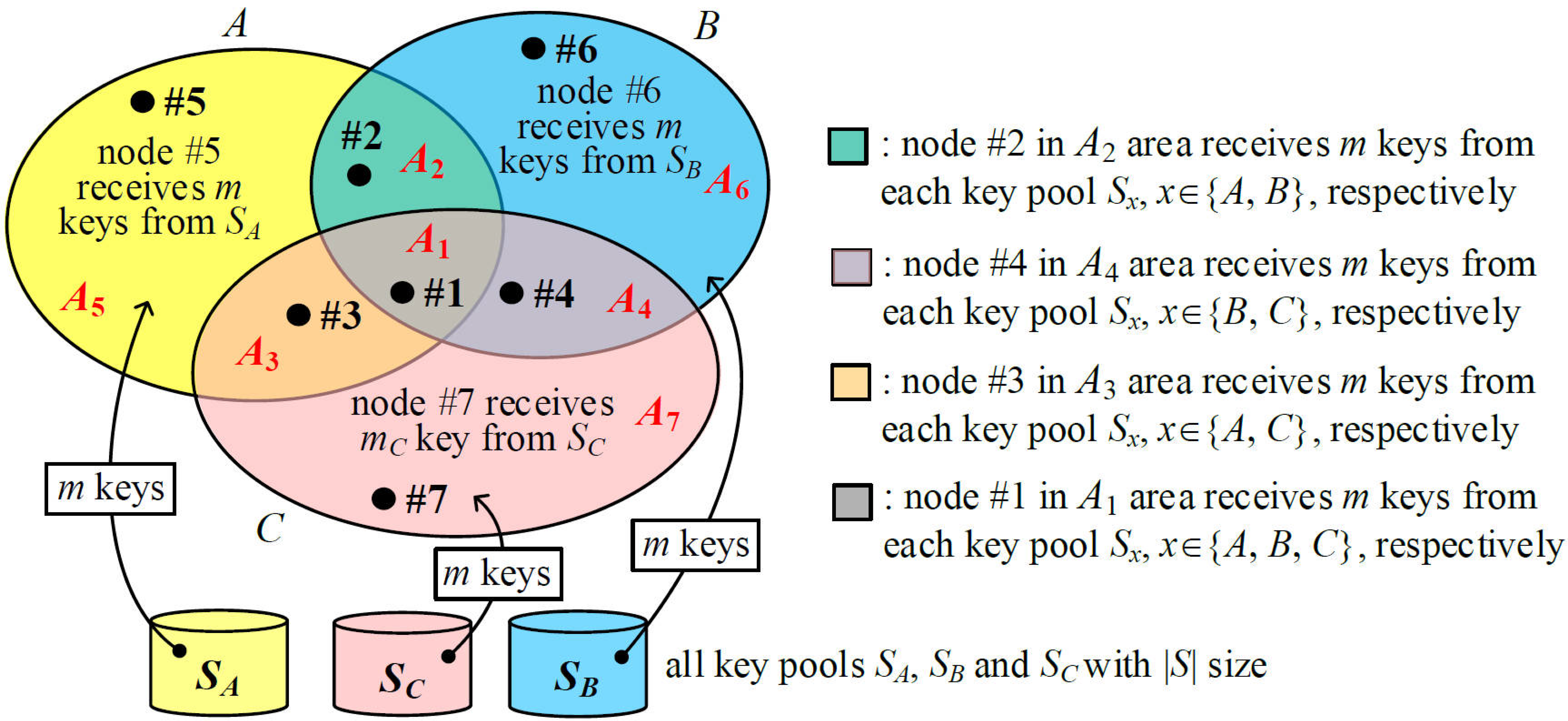
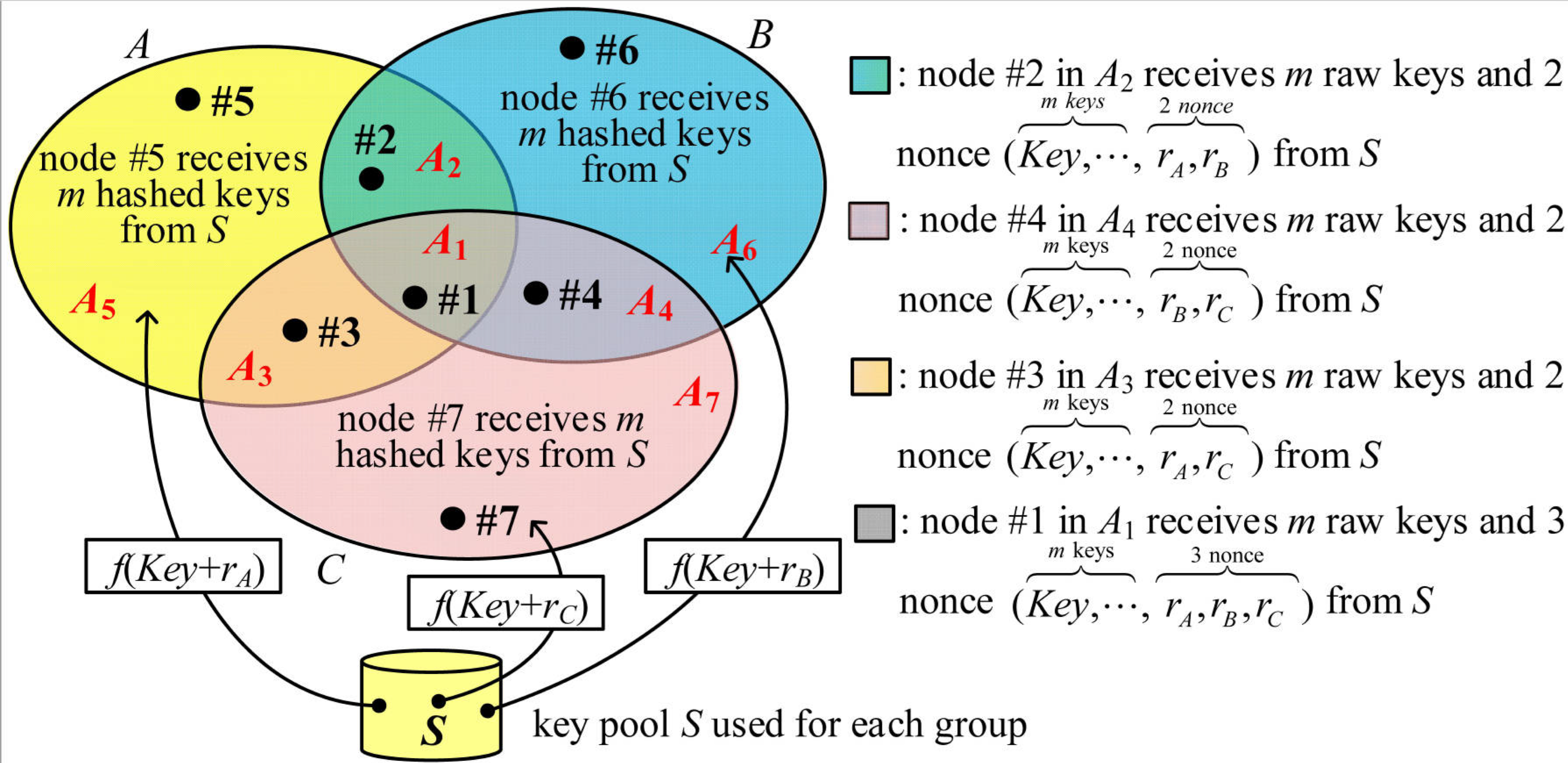
Figure 3 illustrates an example of three groups,
A, B, and
C. Suppose that the number of all possible key rings of size
selected from a key pool
of size
with no identical keys in the key rings, where
x∈{
A,
B,
C}, i.e.,
,
, and
The key selection rules for I
2KPDP are described below. For a node in group
x,
keys are randomly selected from the key pool
. Thus, if the node is in the group
, there are a total of
keys in its key ring. Obviously, the node in the group
will have
keys. For simplicity, we use
and
to describe I
2KPDP. Seven disjointed areas
Ai, 1 ≤
i ≤ 7, with a size of
in
Figure 3 are represented in Equation (1). Finally, nodes #5, #6, and #7 in areas
A5,
A6, and
A7 have a key ring size of
m. Nodes #2, #3, and #4 in areas
A2,
A3, and
A4 have a key ring size of 2
m, while node #1 in the
A1 area has a key ring size of 3
m.
Via [
6,
7], we could derive Equation (2) expressing the probability that any two nodes in the network group
x ∈{
A,
B,
C} share exactly
l independent keys from the key pool
, where
.
Let
be the probability that any two nodes in (
) share exactly
l independent keys and
be the probability that any two nodes in (
) share exactly
l independent keys. Based on Equation (2),
and
are derived in Equation (3), where
.
Obviously, any two nodes in
x,
, and
may share the common keys from the key pools
,
, and
, respectively. The following shows how any two nodes in the whole group
share the common keys. However, if one node is in
x and the other node is in
, they could only use the common key pool
.
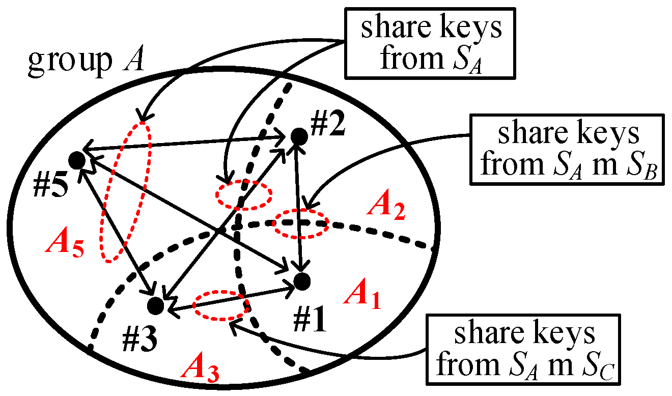
Figure 4 shows the cases between subgroups in group
A.
The links , , , and use the keys from , while the links and use the keys from and , respectively. Because we use the condition and , we have and . To more simply denote the probabilities, we use , , and to represent the probabilities for single-intersected, double-intersected and triple-intersected groups, respectively (note: is the same as that in the conventional KP). The probabilities , , and using the keys from , , and , respectively, share exactly l independent keys for I2KPDP as derived in Lemma 1.
Lemma 1. The intragroup probabilities , , and for I2KPDP, as shown in Figure 2, are derived in Equations (4), (5), and (6), respectively. Proof. As illustrated in
Figure 3, we consider that one node
i in
,
,
, and
(note:
), respectively, and one node
j in
A to communicate with each other (see
Figure 4). All the possible choices of nodes
i and
j in
A are
. Finally, the average probability
is derived as follows.
By the same argument,
and
are derived in Equations (5) and (6).
Based on , the probability that two given intragroup nodes establish a secure link is , where x, y, z∈{A, B, C}. Next, we prove that our I2KPDP satisfies the intragroup and intergroup conditions. □
Theorem 1. The proposed q-composite I2KPDP in Figure 3 satisfies intragroup and intergroup conditions. Proof. We first prove that
q-composite I
2KPDP satisfies the intragroup condition. In each group, we have the probability
,
, and
to establish a secure link. The link connectivity is the same as the connection like in KP. Since the nodes in more intersecting groups have a higher probability of establishing a link, we consider the node in single-intersected (the nodes in
A5,
A6, and
A7), double-intersected (the nodes in
A2,
A3, and
A4), and triple-intersected (the nodes in
A1) groups. Let
, where
, be the set of subgroups that the nodes in
could establish a secure link with the nodes in this set. Obviously, Equation (7) implies that the nodes in more intersected groups can establish a link with more nodes in the whole group
G.
Next, we prove the intergroup condition. The nodes in the two groups
A and
B obtain the keys from key pools
and
, respectively, where
. Thus, the nodes in group
A and the nodes in group
B cannot establish secure links except in the intersected group
. The above implies that the proposed I
2KPDP satisfies intragroup and intergroup conditions. □
The resiliency against NAs for our I
2KPDP is described as follows. I
2KPDP dealing with one group is reduced as in conventional KP. We first show NA resiliency for conventional KP and then give a formal analysis of our I
2KPDP. Suppose that
k nodes are captured in a random fashion, and the stored keys are compromised. Because each node contains
m keys, the probability that a given key is uncompromised is
. On the contrary, the probability that a given key has been known is
. If the key of a link between two nodes is the hybrid of
l shared keys, the probability of that link being compromised is
. Then, the probability that any secure link between two uncompromised nodes is compromised when
k nodes are captured in group
x is calculated in Equation (8), which is the same as in KP [
6,
7].
For the proposed I2KPDP, the nodes in different areas have a different number of keys in their key rings. Thus, we should give different analyses for the probability that any secure link between two uncompromised nodes in is compromised when k nodes are captured. For k captured nodes, it is not reasonable to consider all k captured nodes are randomly distributed in the large-scale MWSN G with many groups (say 200 groups). The case “k captured nodes” in such a large-scale G does not work for an NA, because there is a very low probability that the k captured nodes are selected from the same key pool. An NA attack does not work in this case. The following scenario about an NA in I2KPDP is more possible and reasonable. The attacker could know the nodes belonging to which group, but he does not know whether the nodes are located in intersected groups. As we know, the probability of I2KPDP is the same as in conventional KP. Therefore, we discuss the probabilities , where x∈{A, B, C}, for I2KPDP that any secure link between two uncompromised nodes is compromised in the whole group G when k nodes are captured in a random fashion in group x. All the probabilities , , and are derived in Theorem 2. To simply represent the probabilities , , and , assume that the intersecting group does not have many sensors (note: this is a reasonable assumption). Suppose , and thus we have . By Equations (4)–(6), the values of are . The result implies that we can use to simply derive , where x∈{A, B, C}.
Theorem 2. In q-composite I2KPDP, when k nodes are captured randomly in groups A, B, and C, respectively, the probabilities , , and of a link being compromised are shown in Equations (9)–(11).
Proof. Suppose that
k captured nodes are selected in a random fashion in group
A. There are a total of
ways to select
k captured nodes. As illustrated in
Figure 3, we consider four cases: (i) all
k captured nodes are in
A1, and there are
types to select
k captured nodes; (ii) all
k captured nodes are in
(i.e.,
), excluding case (i), and there are
types to select
k captured nodes; (iii) all
k captured nodes are in
(i.e.,
), excluding case (i), and there are
types to select
k captured nodes; (iv) all
k captured nodes are in group
A, excluding cases (i), (ii), and (iii), and there are
types to select
k captured nodes. The total number of these cases is
. For case (i), the captured keys from
SA,
SB, and
SC can be used to compromise the links in groups
A,
B, and
C. By the same argument, when
k nodes are captured for cases (ii) and (iii), the information of captured nodes can be used for compromising the links in
A and
B as well as
A and
C, respectively. The case (iv) is to compromise the links in group
A excluding cases (i), (ii), and (iii). By the approximation
and the derivation of
in Equation (8), the probability
is approximately derived in Equation (12). This probability is divided by three because the size of the whole set
G is about three times the size of group
A, i.e.,
. By the same argument, we could derive
and
in Equations (10) and (11).
I2KPDP that adopts different key pools for different groups increases the key ring size. Sensor nodes in the intersected groups and must store 2m and 3m keys in the key ring, respectively. To reduce the storage sizes of sensors in intersected groups, we use the same key pool for all groups to design I2KPSP. □
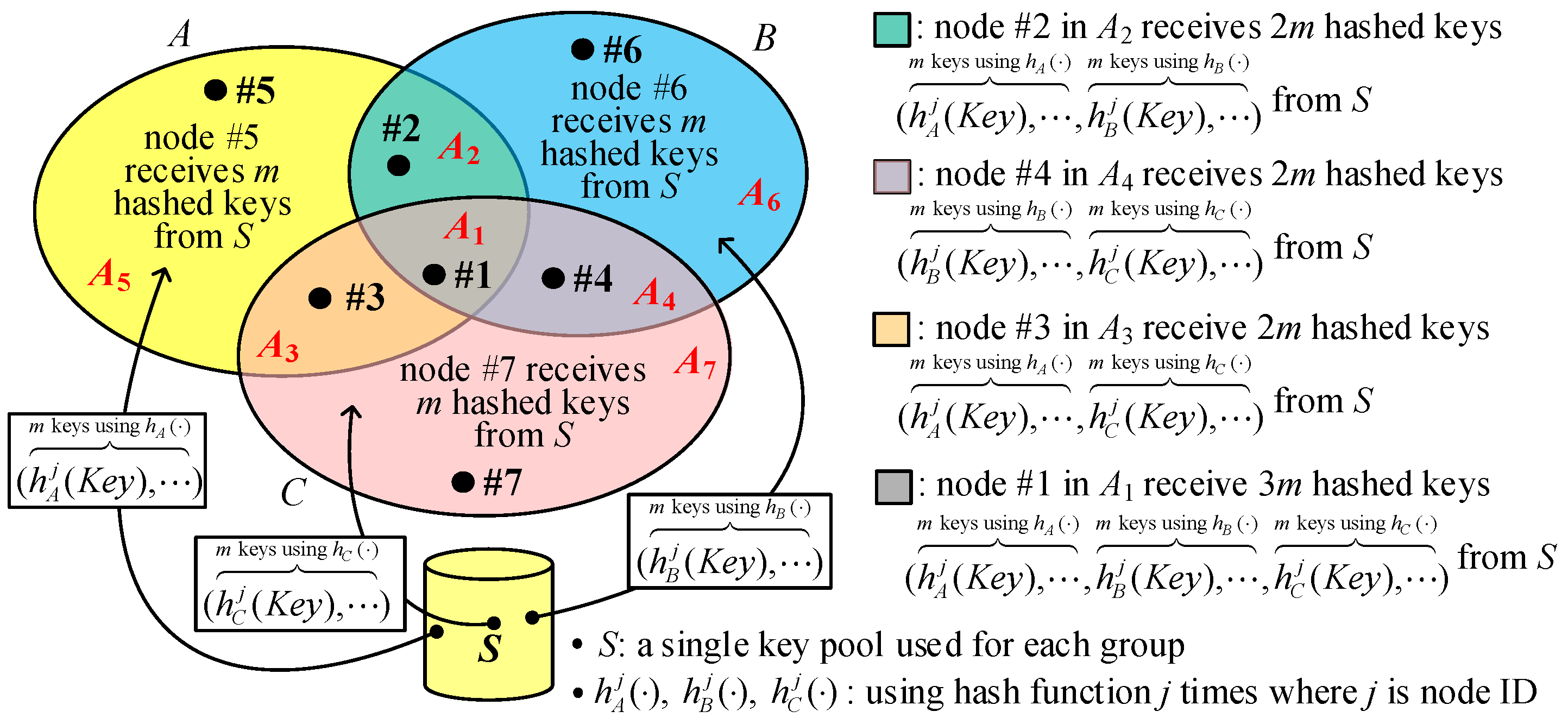
4.2. The Proposed I2KPSP
The same key pool is used for all groups to reduce the key ring size. We also use three groups,
A,
B, and
C, to describe I
2KPSP (see
Figure 5). For the key selection rules in I
2KPSP, a nonce is randomly selected for a group. As illustrated in
Figure 5, three nonces,
rA,
rB, and
rC, and one hash function
are used in I
2KPSP. For the nodes in
, where
x,
y,
z∈{
A,
B,
C}, if
m keys (say
) are randomly selected from key pool
S, then
m hashed keys
are delivered to this node. For the nodes in
, (
m + 2) values including
m raw keys and two nonce
are given to the nodes, while the nodes in
receive (
m + 3) values including
m raw keys and three nonces
. Finally, as shown in
Figure 5, nodes #5, #6, and #7 in areas
A5,
A6, and
A7 have a key ring of size
m; nodes #2, #3, and #4 in areas
A2,
A3, and
A4 have a ring size of (
m + 2); and node #1 in area
A1 has a key ring size of (
m + 3). However, the key ring sizes of I
2KPDP are 3
m for
A1 and 2
m for
A2,
A3, and
A4.
Suppose a key with an identifier ID is selected from S given to a node. If node #a exists in the group , the node will receive the hashed key . Suppose another node is also in . It may share the common key with node #a if it also has the same hashed key from key pool S. Consider the case that node #b is in , , or and has a key with the same identifier. It receives the raw key with the nonce , , or . For these cases, node #b has the nonce , and it can calculate the hashed key to share the common key with node #a. In I2KPSP, we use an extra nonce to share the pairwise key between nodes.
In the same group
x, both nodes share exactly
l independent keys from the key pool
S that have the probability
like in I
2KPDP. Suppose two nodes in the intersected group
have one same key
; they could have the hashed keys
and
for establishing links. Thus, the probabilities that two nodes have exactly
l independent keys in intersected groups are
, on which the
and
of I
2KPSP are derived in Equation (13).
Same as I
2KPDP, we use
,
, and
to represent the probabilities for single-intersected, double-intersected, and triple-intersected groups. Then, for our I
2KPSP, we can get
,
, and
using the keys from the same key pool
S with different nonces
,
, and
. Consider the same case
in I
2KPDP. The
for I
2KPSP is derived in Equation (14), which is approximated to
We can also prove that I
2KPSP satisfies intragroup and intergroup conditions, and we calculate the probabilities of a link being compromised:
,
, and
(same as Theorem 2). Although I
2KPSP does not use a hash chain, it uses a hash function
f(·) to generate hashed keys in the area
. We use the approximation
in Lemma 1, i.e., we do not consider the intersected groups
. For
, we have
. This implies the fractions of intersected groups
and
are very small. In fact, there is already a large portion
in Equation (14) for
, and thus we consider using
only. Four cases using
in group
A as deriving
are (i) node
i in
and node
j in
, (ii) node
i in
and node
j in
, (iii) node
i in
and node
j in
, and (iv) node
i in
and node
j in
A. Two hash operations are required when nodes
i and
j are in
and
, respectively. Note: even though two nodes have raw keys, we use a hashed key to establish a link for keeping consistency in the whole group. The above concludes that the average number of hash operations per node to share a common key in group
A is
(see Equation (15)).
By the same argument, the average numbers of hash operations are
and
for groups
B and
C. Each node in group
x performs the hash function
f(·) an average of
times on all the
l shared keys where
l ≥
q. Since
is the probability that an established link is secured with
l keys for a single-intersected group, the total average number
of hash operations in group
x for
q-composite I
2KPSP is calculated in Equation (16).
I2KPDP and I2KPSP do not have resiliency against LNAs, since attackers may know the nodes belong to the intersected groups from their locations. By an LNA, attackers could intentionally capture k nodes in the intersected groups A1, A2, A3, and A4. Theorem 3 shows all the probabilities , , and greater than , and this means that an LNA is more severe and damaging than an NA. When compared with the case where k nodes are captured in a random fashion in group A, the captured nodes in the intersected groups A1, A2, and A3 aggravate the NA attack.
Theorem 3. In q-composite I2KPDP and I2KPSP, when k nodes are captured randomly in the intersected groups , , and (i.e., using LNA), the probabilities , , and of a link being compromised are greater than the probability .
Proof. Suppose
k captured nodes are in
, and there are
types to select
k captured nodes. Because of using an LNA, attackers could capture all these
k nodes in
. Thus, based on the notion of Equation (12), we can derive
,
, and
as follows.
Via Equation (12), we have
. Since
,
, and
,
. Finally, we have
,
, and
greater than
. □
The above demonstrates that I2KPDP and I2KPSP do not have resiliency against LNAs. In addition, for I2KPSP, the nodes in intersected groups store the nonce in plaintext type. The attacker can capture only one node to obtain the nonce. Thus, if an attacker compromises one node in area A1 to get rC, he can capture nodes in A2 for raw keys and then compromise the link in group C with the compromised raw keys in A2. To effectively tackle LNAs and solve the above problem in I2KPSP, we adopt a hash chain to design I2KPHC.
4.3. The Proposed I2KPHC
We adopt the hash chain approach in [
7] and, in the meantime, give the nodes in intersected groups the large node identifier “
j” to resist LNAs, where 1 ≤
j ≤
n and the value
n is the group size (the number of nodes for each group). In fact, we can use different key pools like in I
2KPDP or a single pool like in I
2KPSP to design the proposed I
2KPHC. When using different key pools, we just need one hash function, while we need different hash functions for different groups when using one key pool. We also use three groups,
A,
B, and
C, to describe I
2KPHC. As illustrated in
Figure 6, we adopt one key pool
S and three hash functions,
,
, and
, for each group to describe our I
2KPHC.
Consider a node with ID “
j” for the following cases: (i) in group
, (ii) in group
, and (iii) in group
, where
x,
y,
z∈{
A,
B,
C}. Suppose
m random keys (say
) are selected from key pool
S, then
m hashed keys
are given to node #
j in group
. There are 2
m hashed keys
and 3
m hashed keys
given to node #
j in the intersected groups
and
, respectively. Finally, as shown in
Figure 5, nodes #5, #6, and #7 in areas
A5,
A6 and
A7 have a ring size of
m; nodes #2, #3, and #4 in areas
A2,
A3, and
A4 have a ring size of 2
m; and node #7 in
A1 area has a ring size of 3
m.
Suppose a key
with an identifier
ID is selected from
S given to a node with node ID “
”. If the node is in the group
, it receives the key
. Suppose another node with node ID “
” is also in the group
; it has
. When
, the node #
applies the hash function
times on
, and then both nodes may share a common key
. Consider other cases for node #
in (i)
, (ii)
, (iii)
, (iv)
, and (v)
. For cases (i), (ii), and (iii), node #
also has
such that it can share the same key
with node #
. However, node #
for cases (iv) and (v) only has
and
, respectively, and thus it cannot share the common key with the node #
. Via the above observations, the approach using the hash function does not affect establishing a link, but it needs extra hash operations when establishing secure links. Although the I
2KPHC in
Figure 6 uses one key pool for all groups, it adopts different hash functions for different groups. All the properties of I
2KPHC are more similar to those of I
2KPSP, because both approaches use one key pool. However, I
2KPHC has the same key ring sizes as I
2KPDP. The probabilities
,
,
,
,
, and
, where
x,
y, and
z∈{
A,
B,
C}, are the same as in I
2KPSP. And, the proposed I
2KPHC also satisfies intragroup and intergroup conditions.
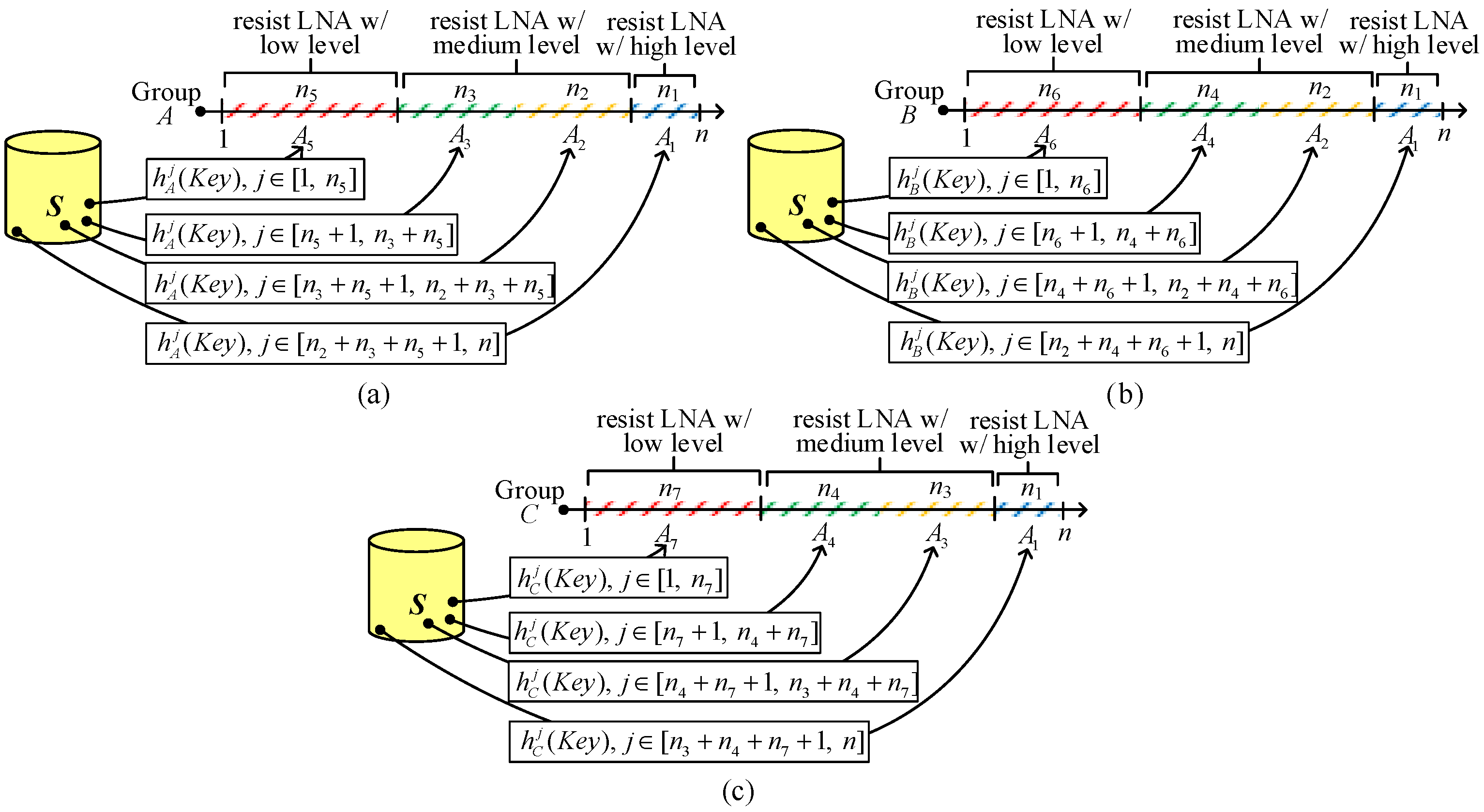
When compared with I
2KPDP and I
2KPDSP, the major difference of I
2KPHC is resiliency against LNAs. LNA resiliency based on the hash chain is described as follows. The diagrammatic representation of key selection rules is illustrated in
Figure 7. The number of nodes for each group is
n (
=
=
=
n). For simplicity, we use 1~
n to represent the node
ID “
j”, where 1 ≤
j ≤
n. How to choose an encoded
ID for sensor nodes for disjointed areas in groups
A,
B, and
C to resist LNAs is given in
Figure 7a–c, respectively.
Consider the key selections for group
A, which is composed of four geometrically disjointed areas (
A1,
A2,
A3,
A5). From I
2KPDP and I
2KPSP, it is observed that the captured nodes in intersected groups, e.g., in
and
, the NA will be seriously aggravated. Therefore, we define three levels of resiliency (high, medium, low) against NAs for the intersected groups:
A1 (triple-intersected),
A2 and
A3 (double-intersected), and
A5 (single-intersected)). We use medium resiliency for
A2 and
A3, because both areas have probabilities of compromised links in
and
, respectively. The reason choosing high resiliency for
A1 is to resist the high probability of compromised links. The key selection for group
A is illustrated in
Figure 7a. We use the
ID to prepare a hashed key
for
, the
ID to prepare a hashed key
for
A2, the
ID to prepare a hashed key
for
A3, and the
ID to prepare a hashed key
for
A5. When the nodes in
A1 are captured, an attacker has the hashed key
, where
, but he cannot obtain the hashed key
for node
in areas
A2,
A3, and
A5 because
. We can also check another situation where if node
is in areas
A2 and
A3 and node
is in area
, both nodes
and
cannot share the common key. This is because
is greater than
. Obviously, node
in
A5 only has the probability to obtain the same hashed key
with node
also located in
A5. By the same argument, we can choose the hashed keys for sensor nodes in groups
B and
C. The key selections for groups
B (including
A1,
A2,
A4, and
A6) and
C (including
A1,
A3,
A4, and
A7) are shown in
Figure 7b,c, respectively.
In [
7], a parameter key-chain length
L is introduced to reduce these hash operations. Each node #
j applies one-way hash operation to their keys
j (mod
L) times instead of
j times, namely storing
instead of
. Finally, the number of hash operations for establishing a pairwise key is bounded by
L. When adopting the notion of key-chain length
L in I
2KPHC to save energy consumption overhead, the key selections in
Figure 7a–c should be a little modified. Here, we only use key selection for group
A to describe the modification. We first define
, where
. The choice of these values can be determined according to the group size
n and the reduction in computation overhead. After the key selection for group
A in
Figure 7a, let the node
ID ,
,
, and
. Next, we figure out the new modified ID
,
,
, and
by Equation (18a). By the same argument, we may choose
for
, and the new modified ID for groups
B and
C are given in Equations (18b) and (18c), respectively.
We herein use the original node ID to more easily analyze the LNA resiliency of our I2KPHC. Actually, both have similar results. Lemma 2 shows the probability that a given key is known in the area when a node is randomly captured in the area . And, the probability , where , is referred to as an improvement in I2KPHC. Since each node has m keys from key pool S, the probability that a key has been discovered in when a node is compromised in is for I2KPHC. Thus, the value implies no improvement from using a hash chain, i.e., the probabilities of compromised links are unchanged. On the other hand, is 0 for . Namely, the approach can completely tackle LNAs. The value ranging from 1 to 0 shows the attack mitigation of LNAs. A hash chain could reduce interception from the attacker, and that is why we call the value “improvement”.
Lemma 2. When using the hash chain class with n ( ) in I2KPHC, the probability is derived as follows.
Proof. For the case with nodes in this area, suppose the node ID in ranges between and . For any hashed key stored in the nodes in , it is initially hashed times, where , with a probability . When a captured node is hashed times, the probability that a key has the same identifier can be figured out is (note: a hash function can only be accomplished forwardly). Thus, the probability to find a key having the same identifier with a compromised node is Consider the case “(node ID j1∈Ai > j2∈Aj) (no same hash function in Ai and Aj)”. Firstly, the condition implies that even though both areas have same hash function , the hashed key cannot be disclosed from . Secondly, both areas with different hash function cannot have the same hashed key. Thus, we have for this case. Consider the other case “(node ID j1∈Ai ≤ j2∈Aj) (one same hash function in Ai and Aj)”. Both areas have the same hash function . Since ≤ , the hashed key can be derived from . This implies . □
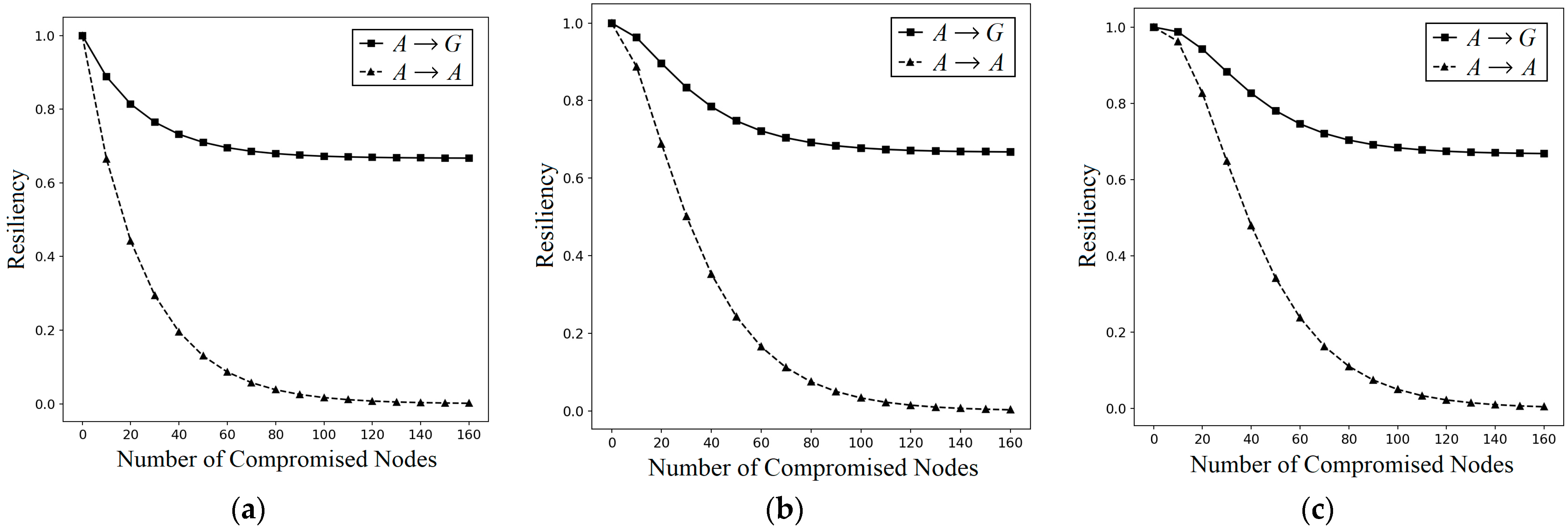
By LNAs, attackers could intentionally capture the nodes in intersected groups (A1~A4) to compromise the links. Consider intersected groups A1, A2, and A3 in group A (note: the analysis for A4 is the same as for A2 and A3 and is omitted here). In Theorem 4, the probabilities , , and of I2KPHC are derived, where and are lesser than those in I2KPDP and I2KPSP, and is almost the same. The result implies that the resiliency of I2KPHC against LNAs is enhanced.
Theorem 4. In q-composite I2KPHC, k nodes are captured randomly in the intersected groups A1, A2, and A3 (i.e., using LNA). When compared with I2KPDP and I2KPSP, I2KPHC has smaller and and almost the same .
Proof. Same as deriving the probabilities in Theorem 3, because there is already a large portion
, we consider using
only. Four cases using
in group
A as deriving
are (i) node
i in
A1 and node
j in
A5, (ii) node
i in
A2 and node
j in
, (iii) node
i in
A3 and node
j in
, and (iv) node
i in
A5 and node
j in
A. In case (i), two nodes can share a hashed key
since
i >
j. Thus, the link may be compromised with the probability
with the improvement
. For cases (ii) and (iii), the improvements
. Case (iv) is subdivided into node
i in
A5 and node
j in
A1, and node
i in
A5 and node
j in (
A −
A1), and the improvement
. Based on the above observations, the probability
that
k captured nodes are in
A1 is derived as follows.
Same as deriving
, we could derive
and
.
. Then, the
is calculated as follows.
For calculating
and
, we first derive
in Equation (22). By the same argument, we also have
,
, and
. Then,
and
are derived in Equations (23) and (24).
For the case using only (a large portion in Equation (4)), and are very small (note: choosing the values is a reasonable choice). Equations (25)–(27) show that the probabilities and of I2KPHC are lesser than those in I2KPDP and I2KPSP, and is almost the same as in I2KPDP and I2KPSP. □
In the proposed I2KPHC, extra hash operations are required to share the common key between two nodes. The following evaluates the computation overhead in our I2KPHC. Similar to deriving the number of hash operations for I2KPSP, we use the approximation and ignore and (it is reasonable for ). We still consider four cases using in group A as deriving : (i) node i in A1 and node j in A5, (ii) node i in A2 and node j in , (iii) node i in A3 and node j in , and (iv) node i in A5 and node j in A. Thus, the average number of hash operations to share a common key is determined in Equation (28).
Similar to deriving , we can figure out and . Finally, in q-composite I2KPHC, both nodes should apply the average hash operations in group x when establishing a secure link.


 #6), node #4 in group B and node #13 in group D (#4
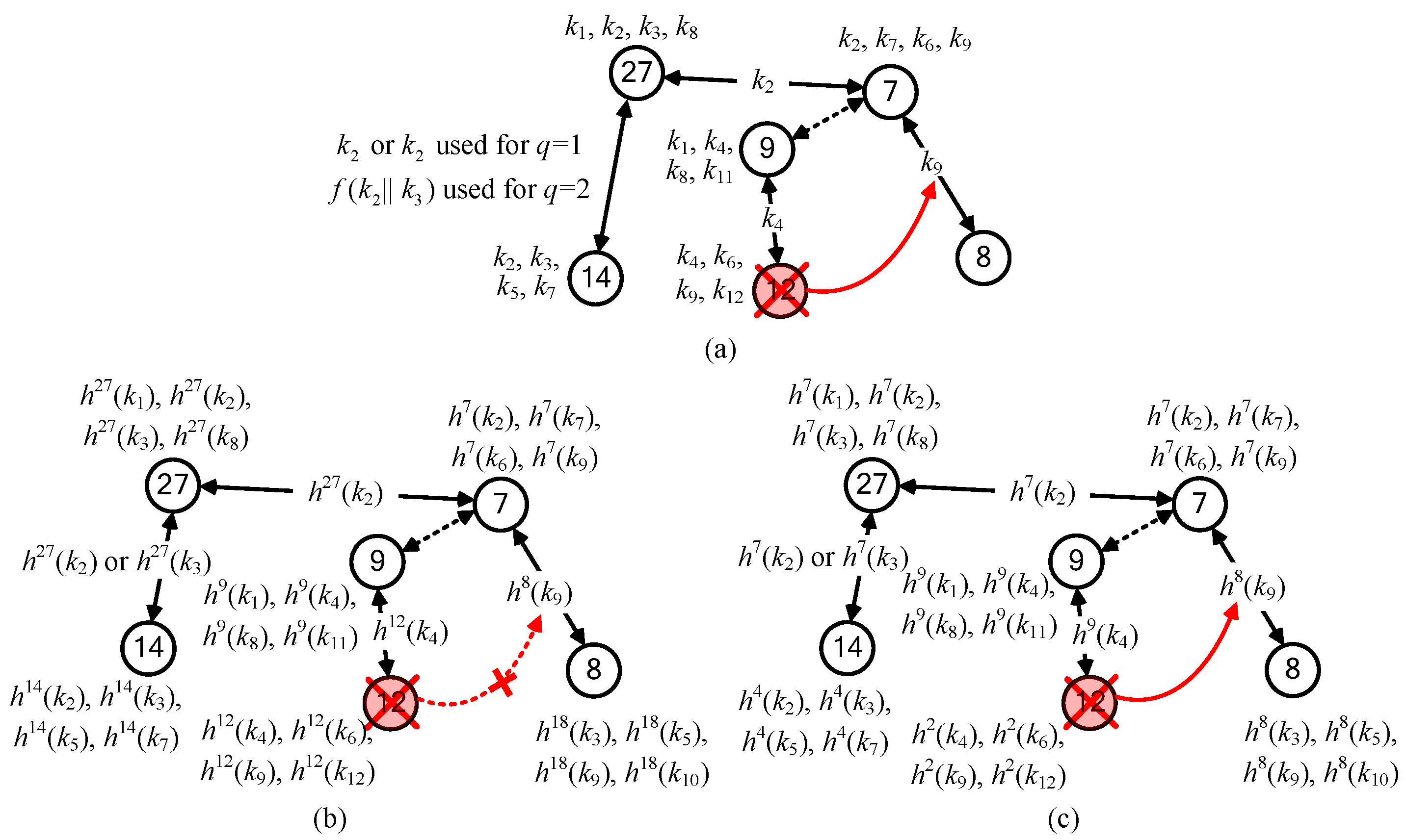
