
A Wireless Data Acquisition System Based on MEMS Accelerometers for Operational Modal Analysis of Bridges


Abstract
1. Introduction
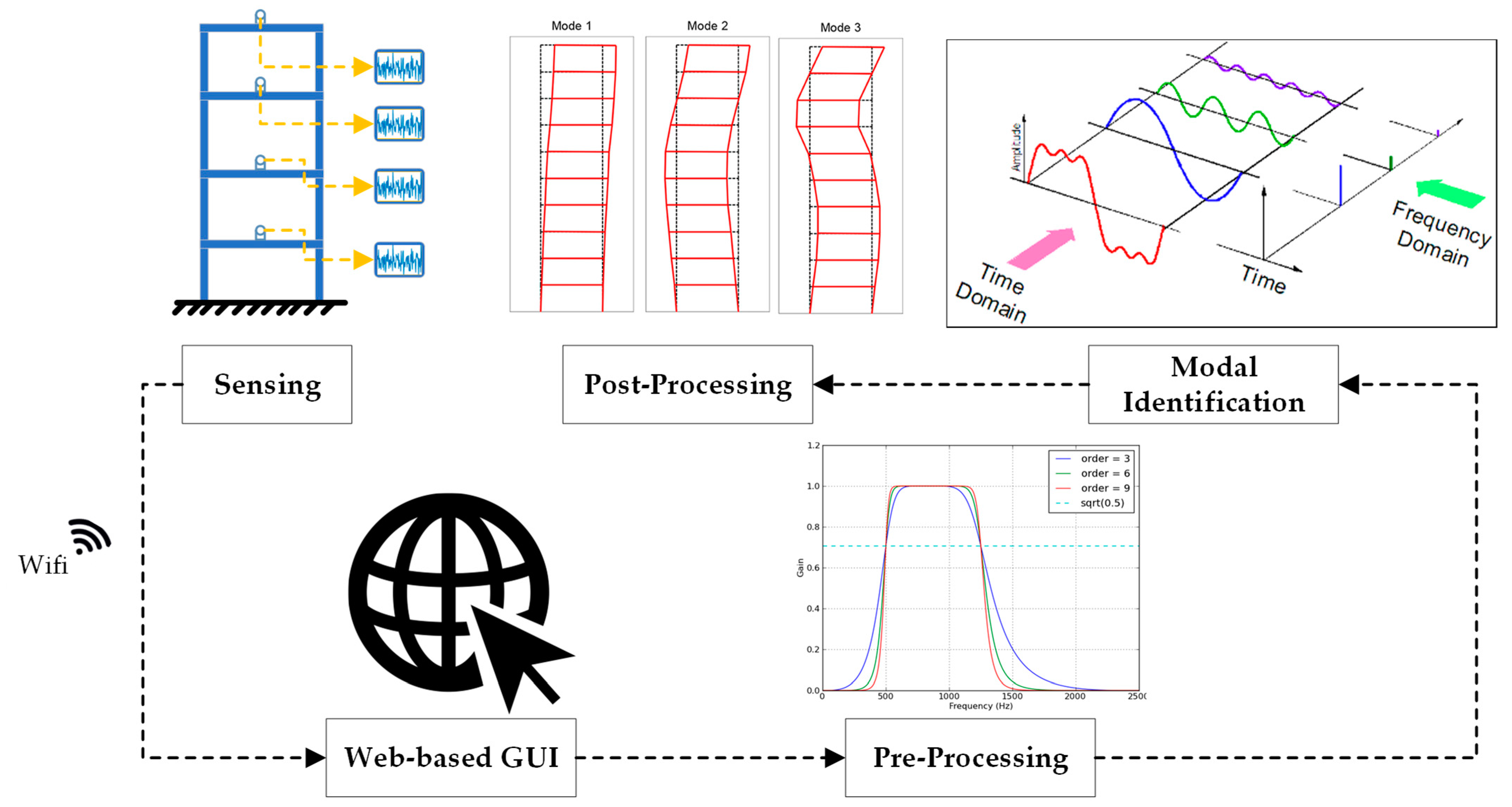
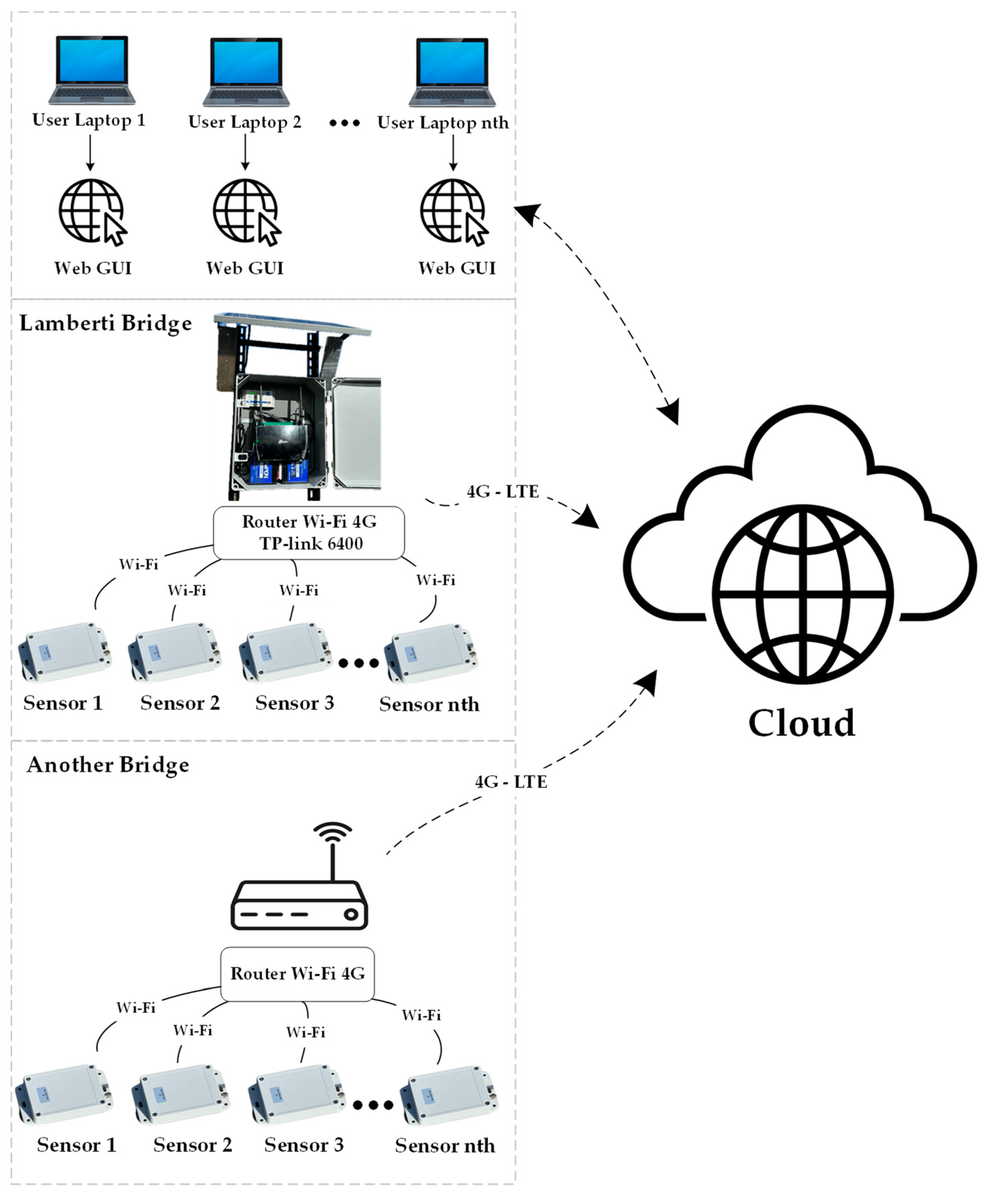
2. Monitoring System Overviews
- Easy configuration is essential and should be accomplished remotely.
- Users should have the capability to configure all sampling parameters, including frequency rate, duration, and starting time.
- It should have the capability to sample continuously for a minimum of one hour at a rate of 125 Hz, which is the amount of data typically required for OMA applications.
- Accelerometer measurements must meet specified criteria for precision, repeatability, and noise levels. This includes ensuring that the frequency range falls within the minimum required frequency and the maximum measurement frequency, avoiding saturation of the instrument, maintaining a minimum signal-to-noise ratio (≥10 dB), and ensuring adequate sensitivity for A/D conversion.
- Data synchronization for modal analysis must be precise: The synchronization error is advisable to be less than 1/10 of the sampling period.
- Connection must be wireless, stable, and reliable.
- It must be reliable and able to operate without external maintenance throughout its life cycle.
- It must be able to work outdoors; all of its components must function at all temperatures, and the enclosure must be weather-resistant.
- The cost of each sensor should be affordable, and the components utilized should be readily accessible.
- To ensure the transparency of the analysis process, it is imperative that data be transmitted and made fully available.
2.1. Sensor
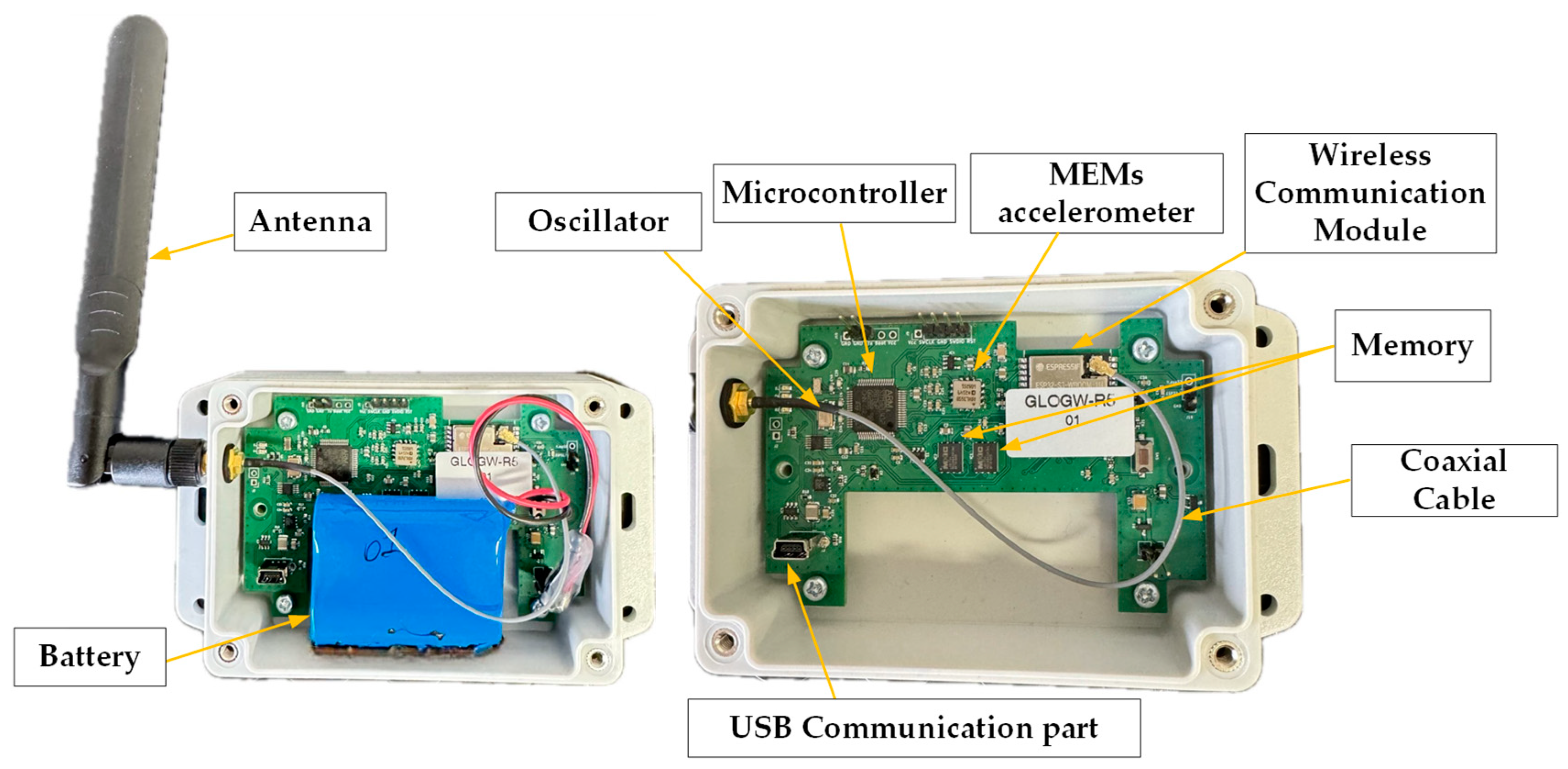
2.1.1. Hardware
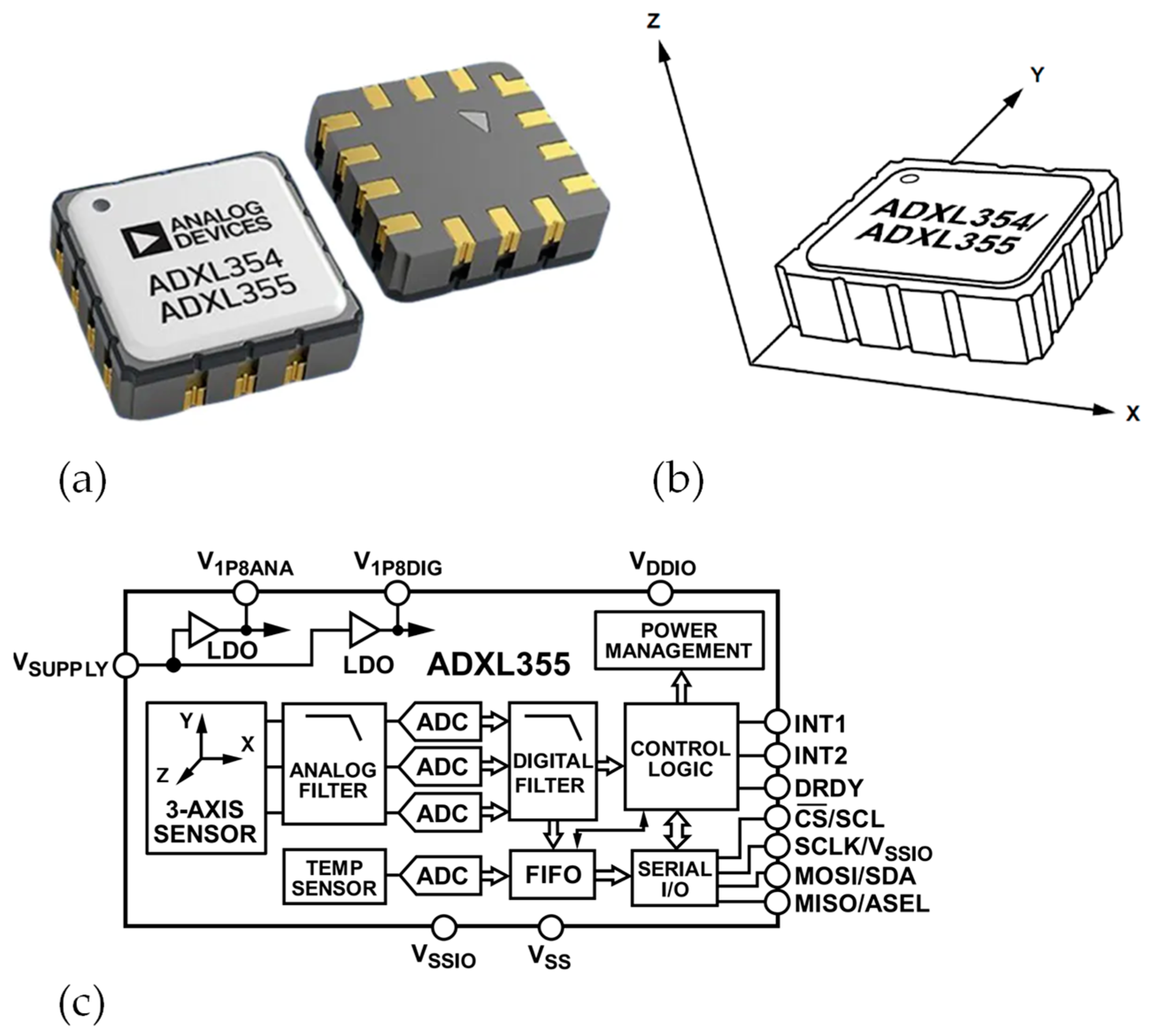
Accelerometer
Wireless Module
- Synchronization
Memory
Host Microcontroller
- Configure the accelerometer and read data.
- Configure the memory, read, and store data.
- Configure the communication module.
- Receive operational configuration from the network and apply it correctly.
- Handle external USB communication.
- Enable the entire board’s power-saving mode, activating other components only when necessary.
- Synchronize and maintain the board’s time base (clock).
USB Communication
- Configuring Wi-Fi network parameters (SSID and password).
- Performing tests to assess the health of the components.
- Downloading data in the event of unavailability of the Wi-Fi network.
- Updating the device firmware.
Battery
- Minimum five-year lifespan: Ensuring a lasting operational period is essential, given that the sensors may be deployed in hard-to-reach and challenging environments. They must supply ample energy to support prolonged monitoring over an extended period.
- 30 min of daily operation: The battery’s lifespan is contingent on the volume of data to be collected. A battery supporting 20 Wi-Fi connections per day will undergo more strain compared to one facilitating a connection once a week.
- 400 mA pulsed capacity: The battery should have the capability to deliver up to 400 mA, which represents the maximum energy demand during a Wi-Fi connection.
Antenna
Enclosure Box
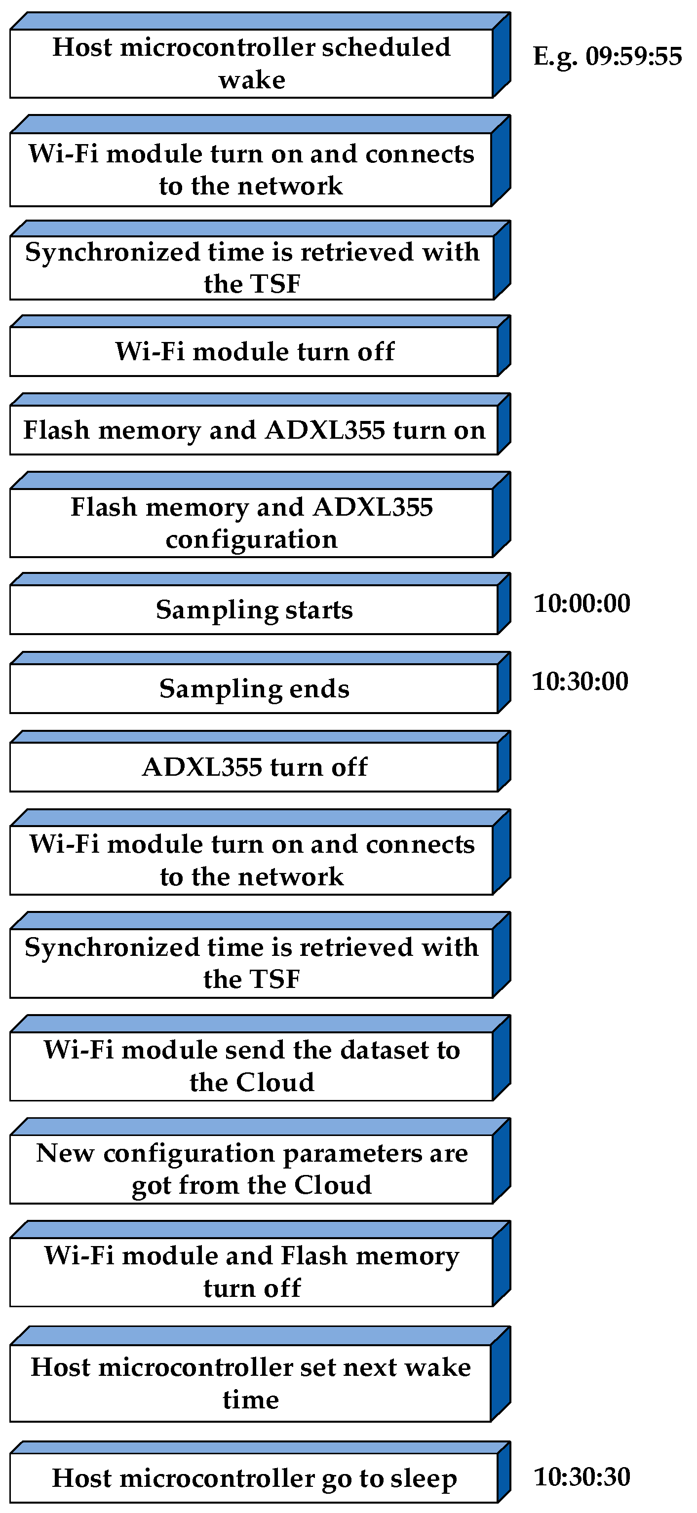
2.1.2. Workflow
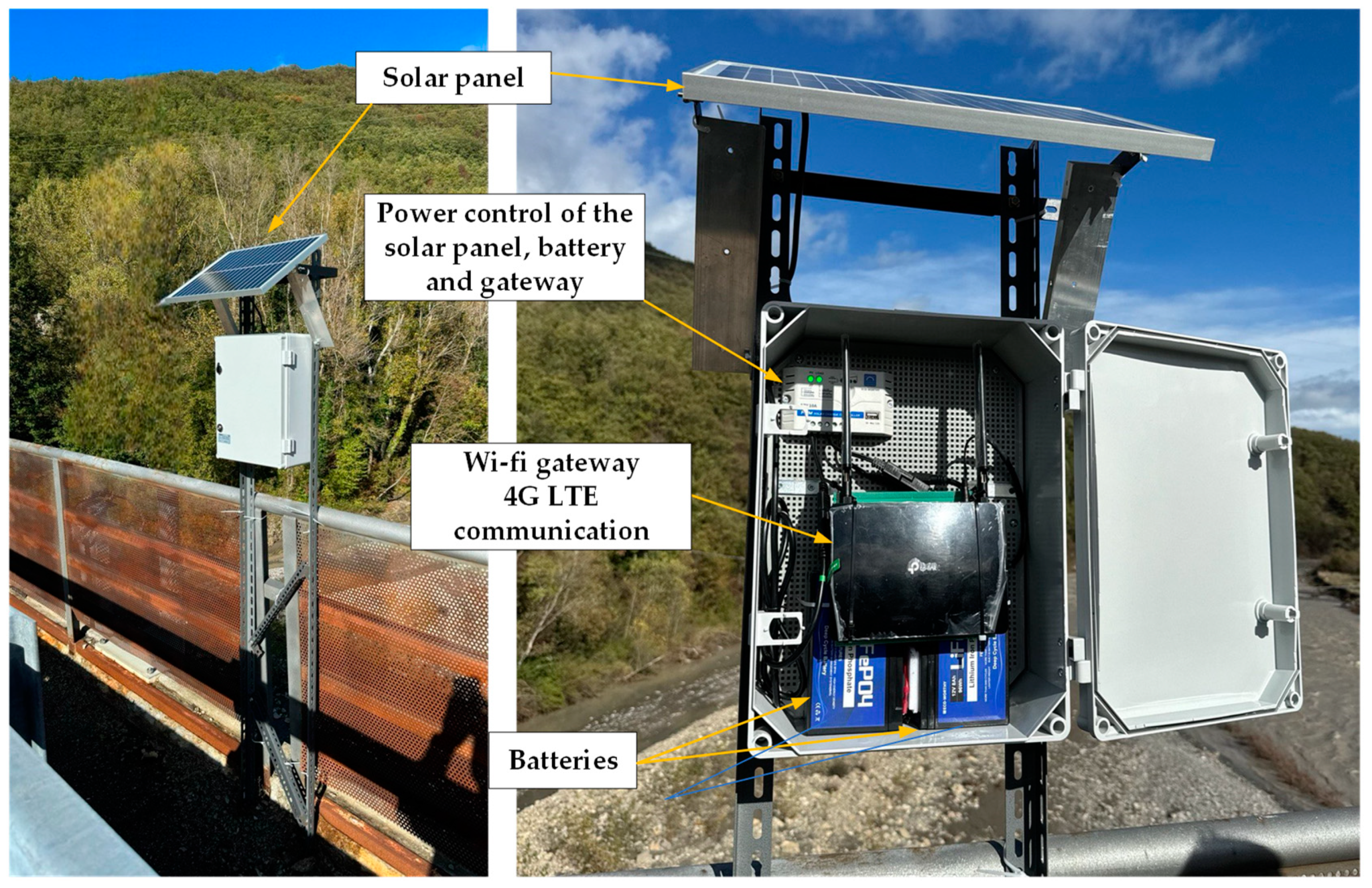
2.2. Router
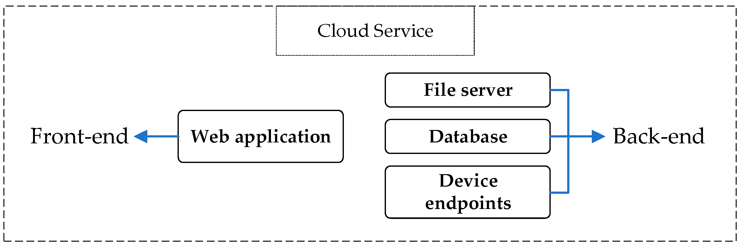
2.3. Cloud Platform
- Device endpoints: These serve as the “addresses” to which the sensors in the field connect for sending data and receiving configuration.
- File server: This is a memory block where data received from devices are stored and sorted by device (using the unique MAC address of the devices as a reference) and timestamp. All data are stored in a super-compressed format to save disk space and are converted into a human-readable format when downloaded. For instance, a 60-min sampling at 125 Hz consists of a 7-megabyte file in compressed format and a 17-megabyte CSV format file.
- Database: This is a structured query language (SQL) database, which consists of highly structured tables. Each row represents a data entity, and each column defines a specific information field. In our case, it is responsible for storing the lists of users, their associated devices, their events, and their functional configurations.
- A page dedicated to user authentication and registration;
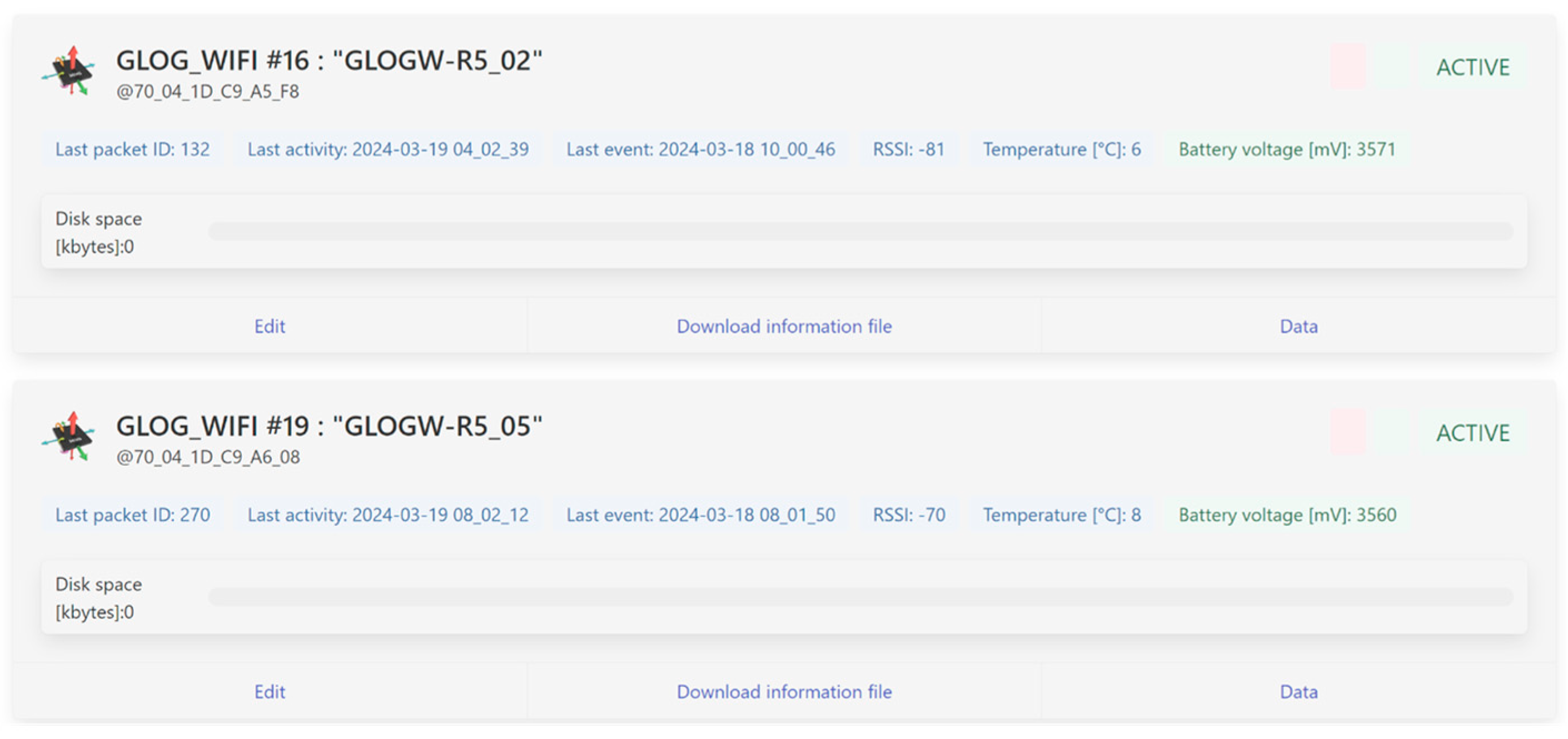
- A device page (depicted by Figure 8) that showcases a list of devices linked to each user, presenting essential details, such as the last connection time, last sampling time, last measured temperature, and battery status;
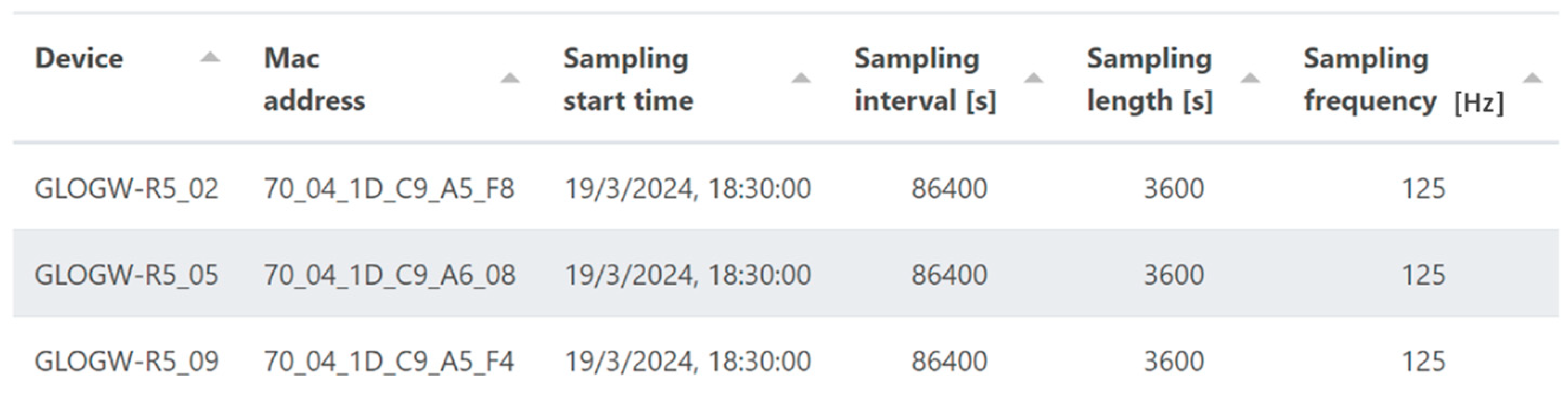
- A configuration page (Figure 9) featuring a table for device configuration. The table is structured in rows, where each row corresponds to a device uniquely identified by a user-set name and its MAC address. Each device can be configured with the following:
- Sampling start time: exact time at which the device should start sampling;
- Sampling interval: time between each sampling, in seconds;
- Sampling period: desired duration of the sampling, in seconds;
- Sampling frequency: frequency at which the accelerometer should operate, in Hz;
- Get config interval: the maximum time between two connections to the server. If set lower than the sampling interval, it allows the sensor to connect to the server to download the configuration without performing the sampling part. This feature allows the system to be more “responsive,” albeit at the expense of battery life.
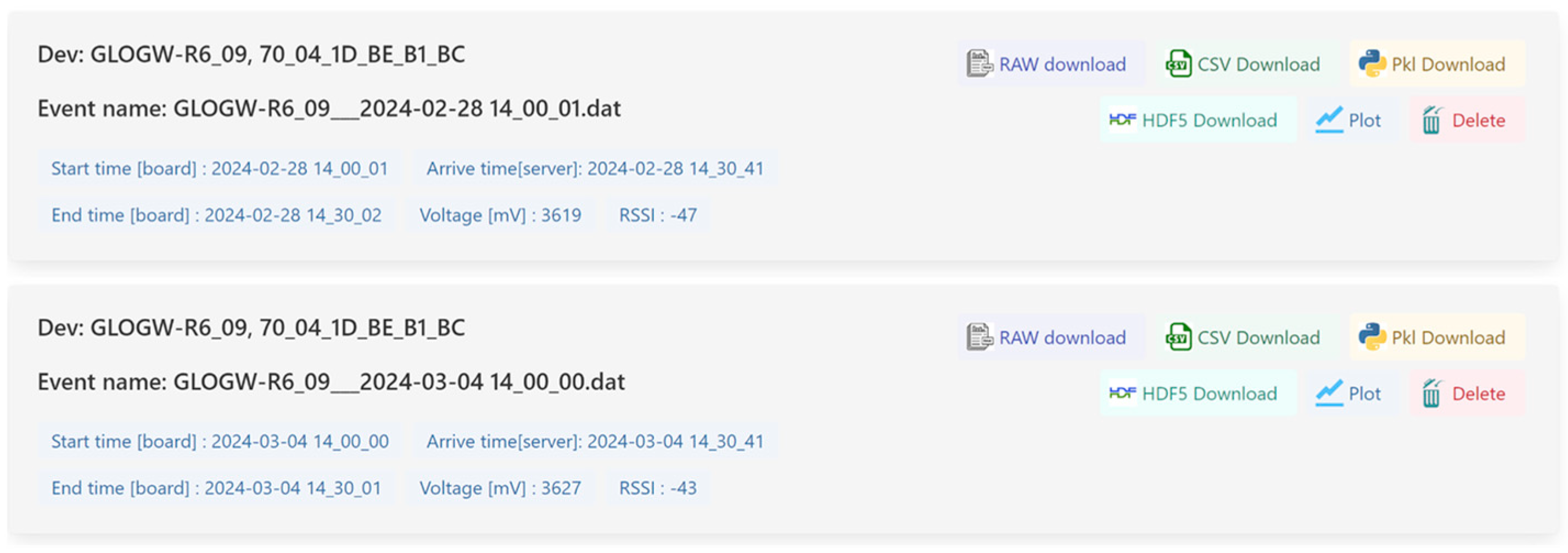
- A file page (illustrated by Figure 10) presents the list of data received from a particular device. Each dataset includes information about the start and end times of the sampling process. Users have the option to download the data in either CSV or HDF5 format.
3. Data Pre-Analytical Process
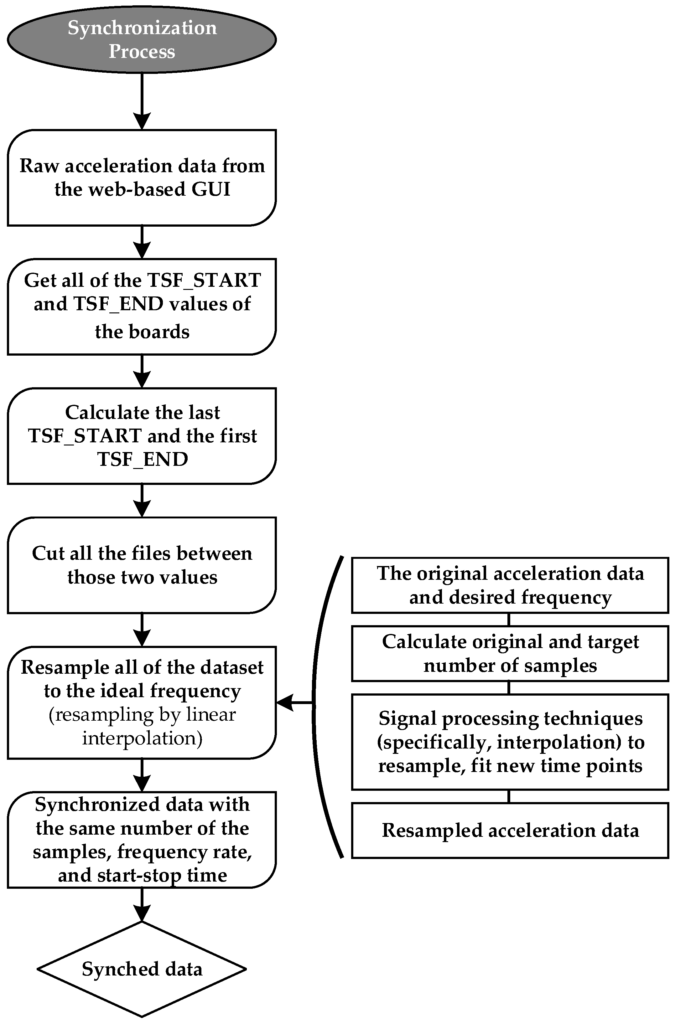
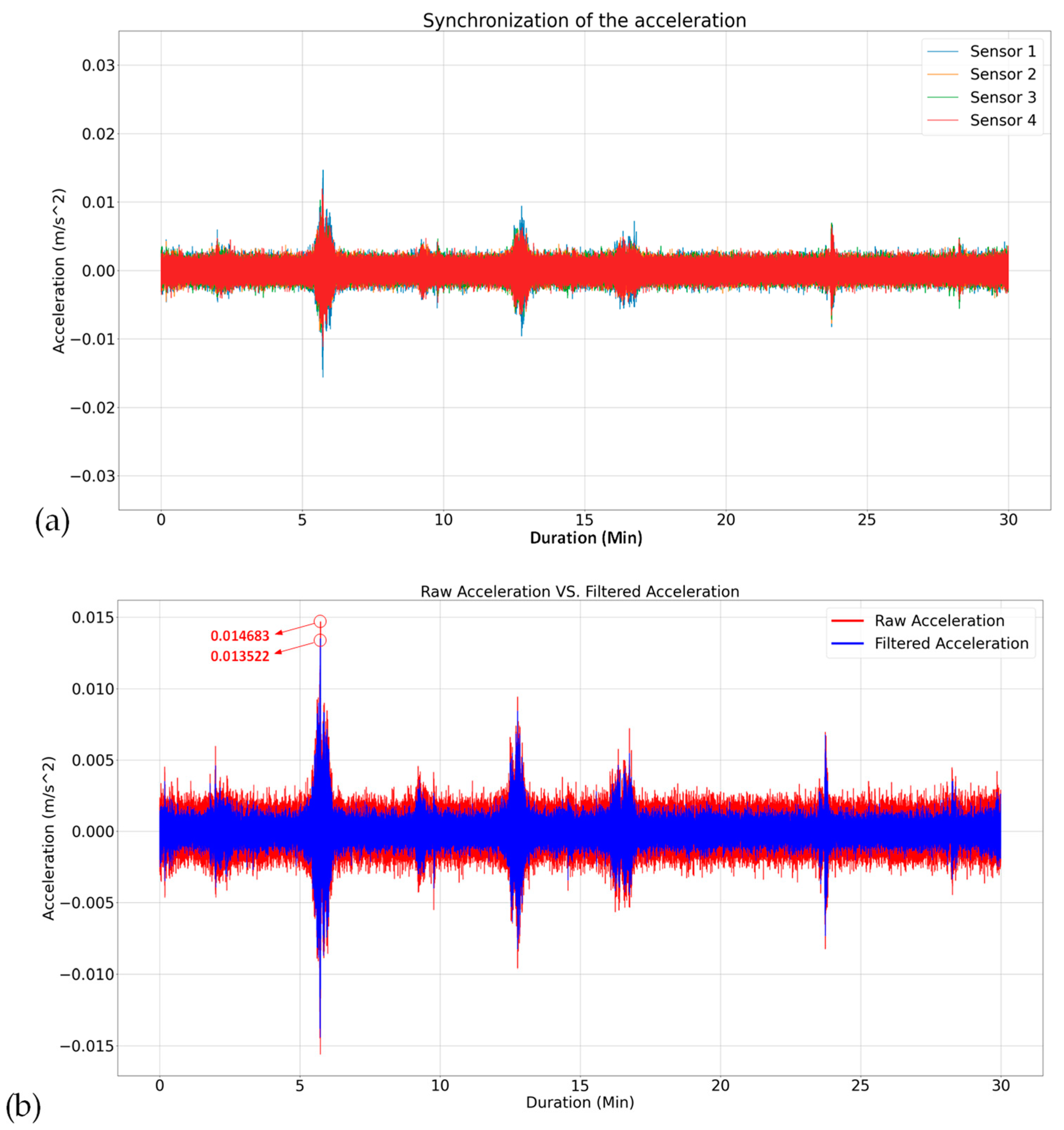
3.1. Synchronization Process
- The commencement times exhibited occasional slight variations.
- The sampling frequency occasionally deviated slightly (e.g., a board sampled at 125.8 Hz instead of 125 Hz).
4. Experimental Process
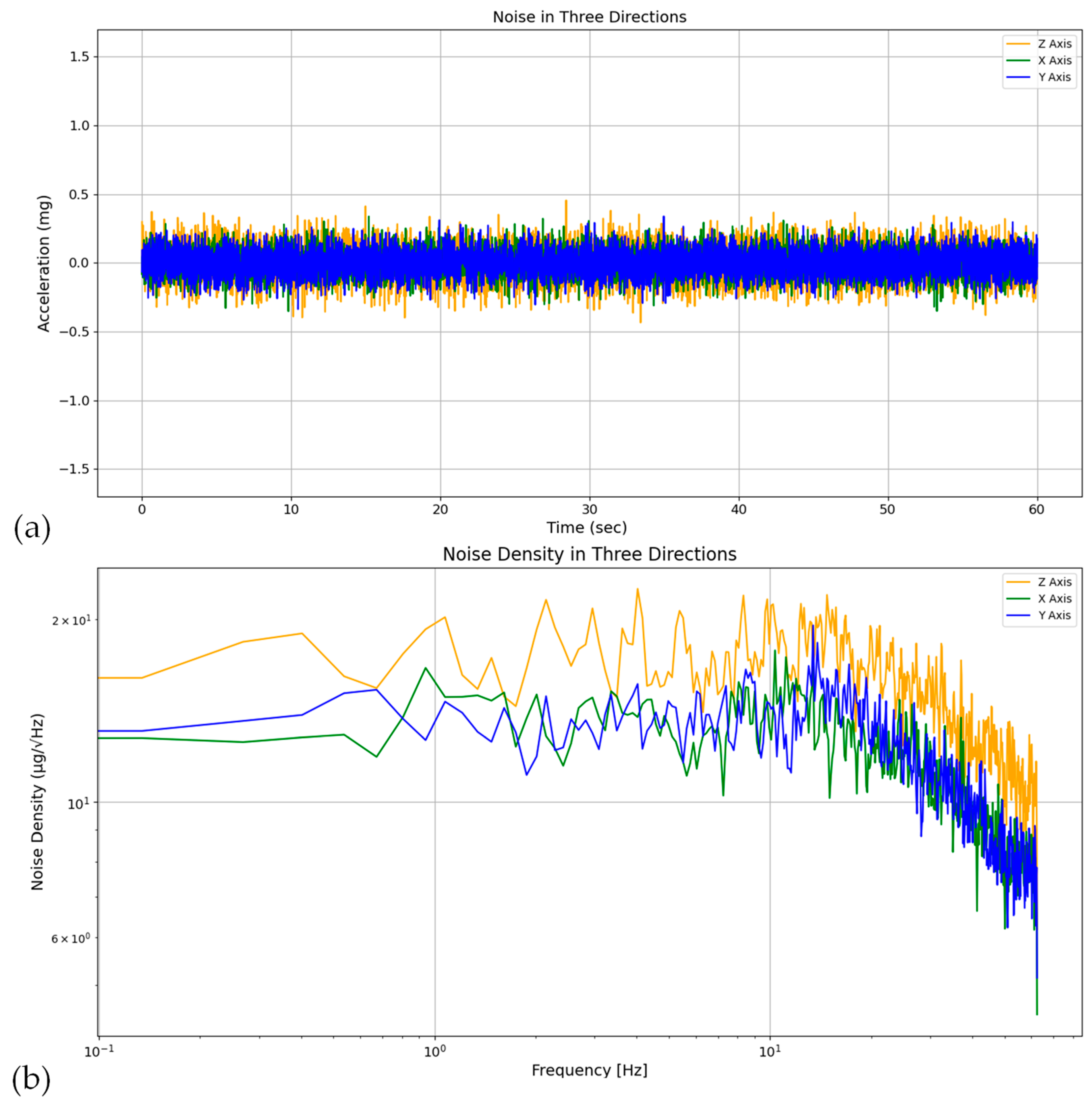
4.1. Sensor Noise Characterization
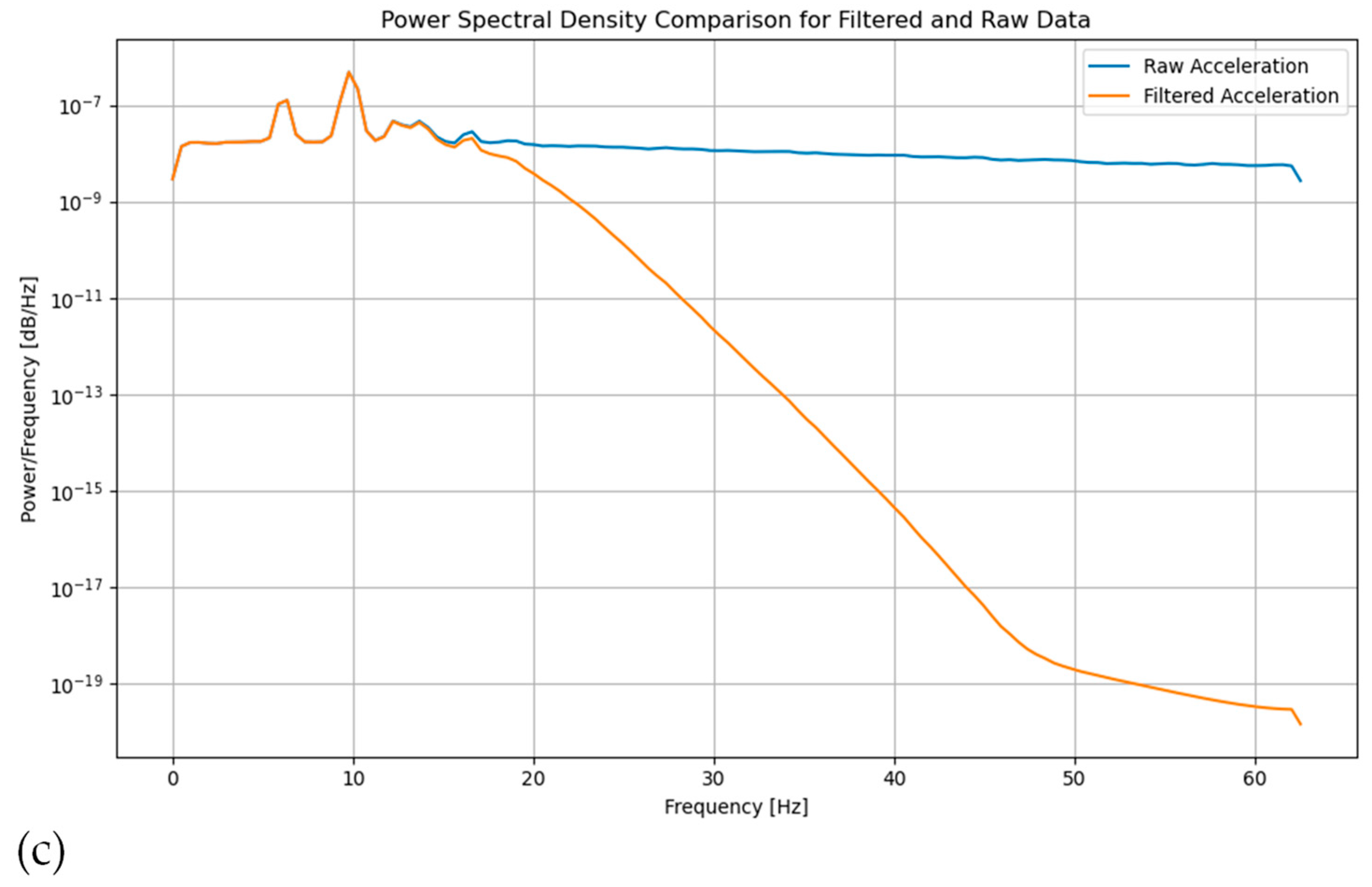
4.2. Preprocessing Step
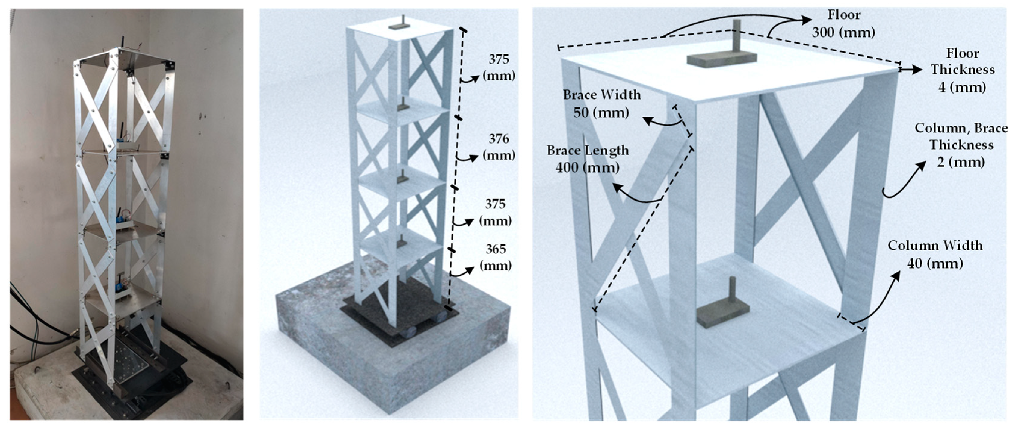
4.3. Laboratory Validation
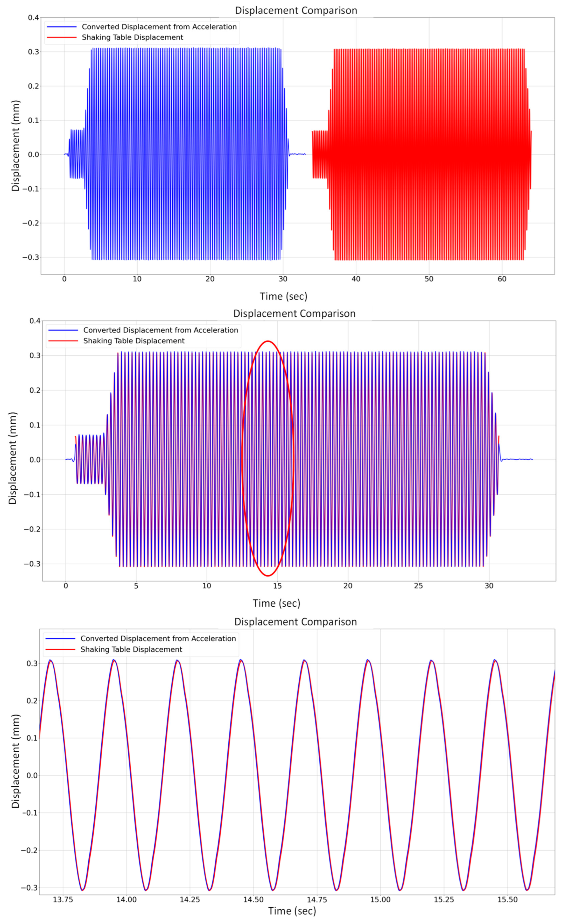
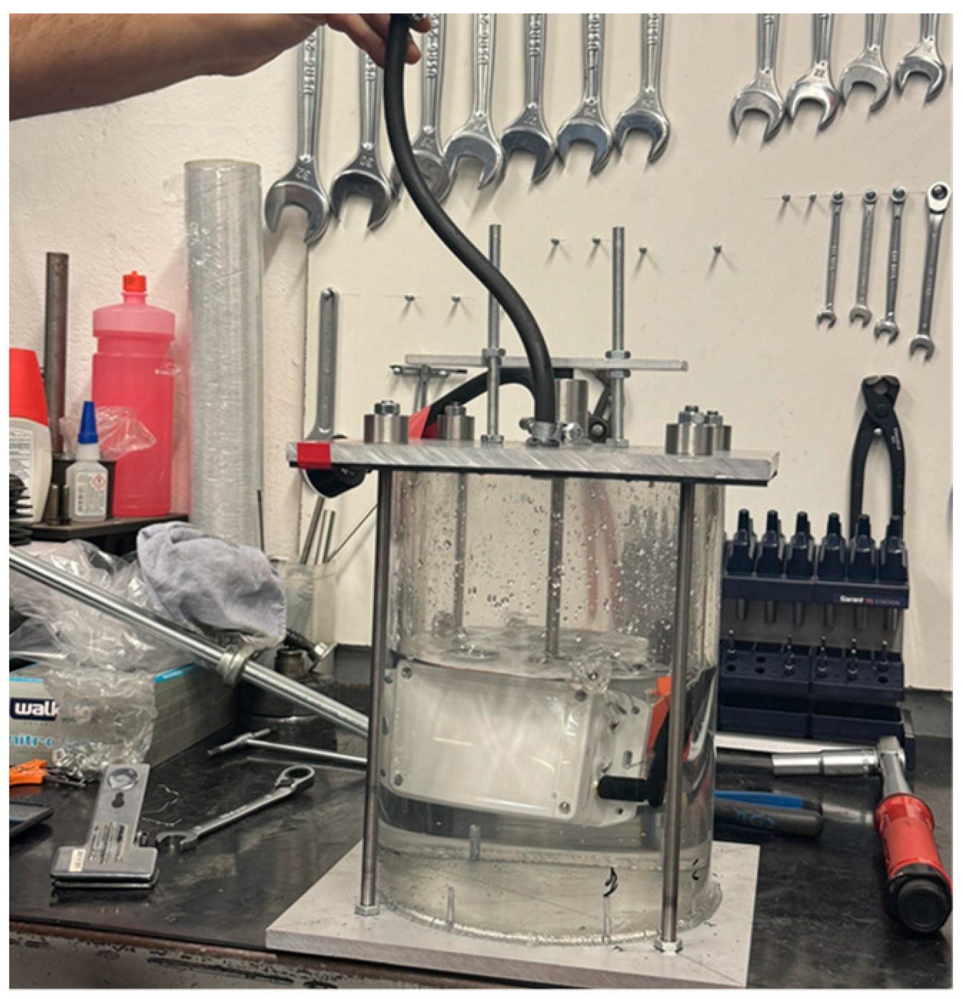
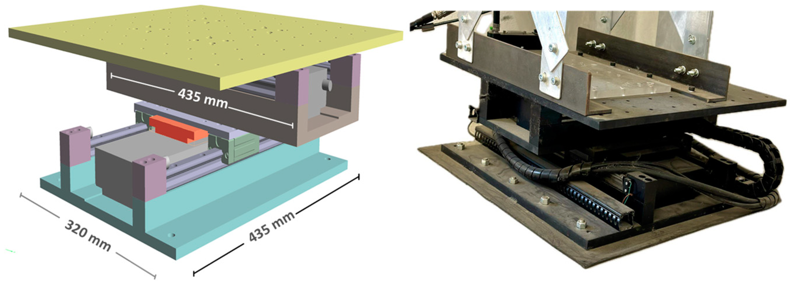
4.3.1. Dynamic Verification against Shaking Table
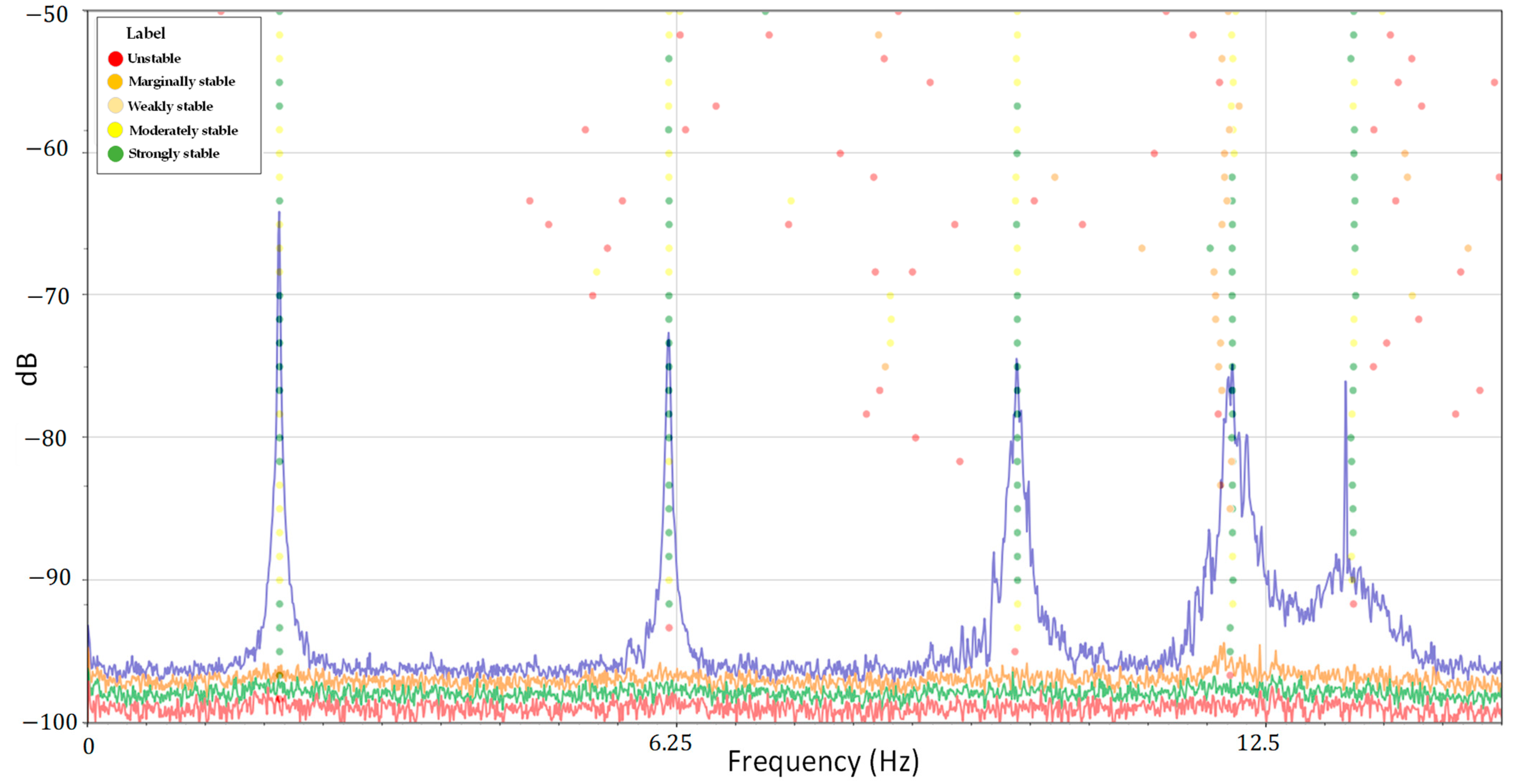
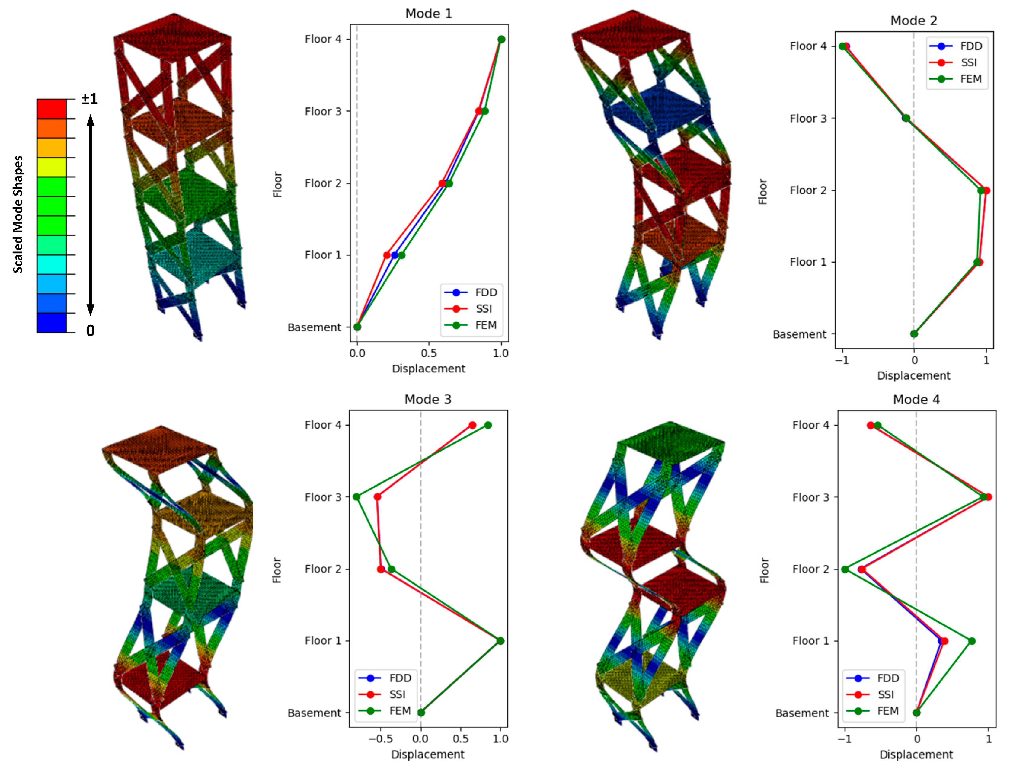
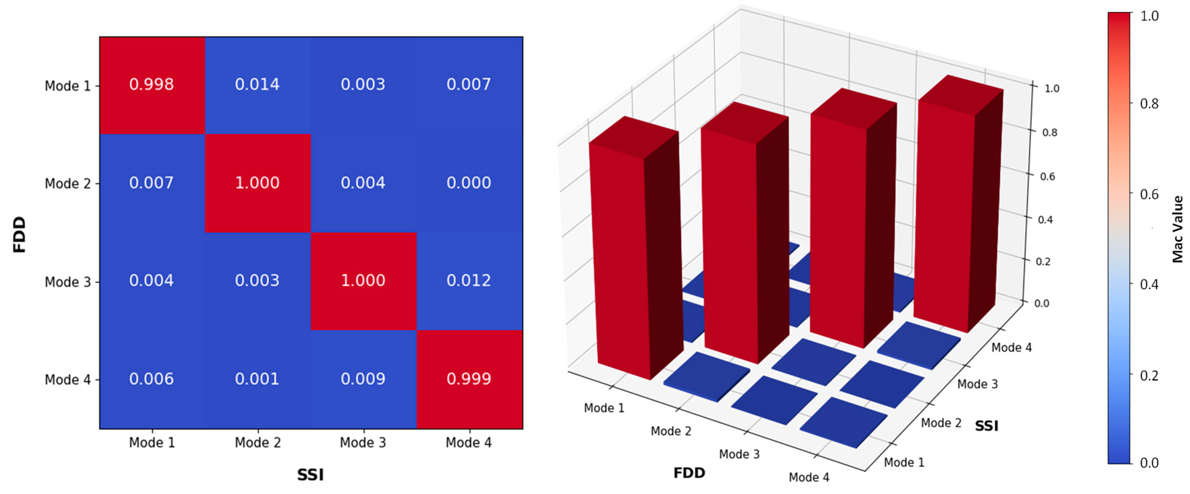
4.3.2. Modal Identification Step
4.4. Real Case Test
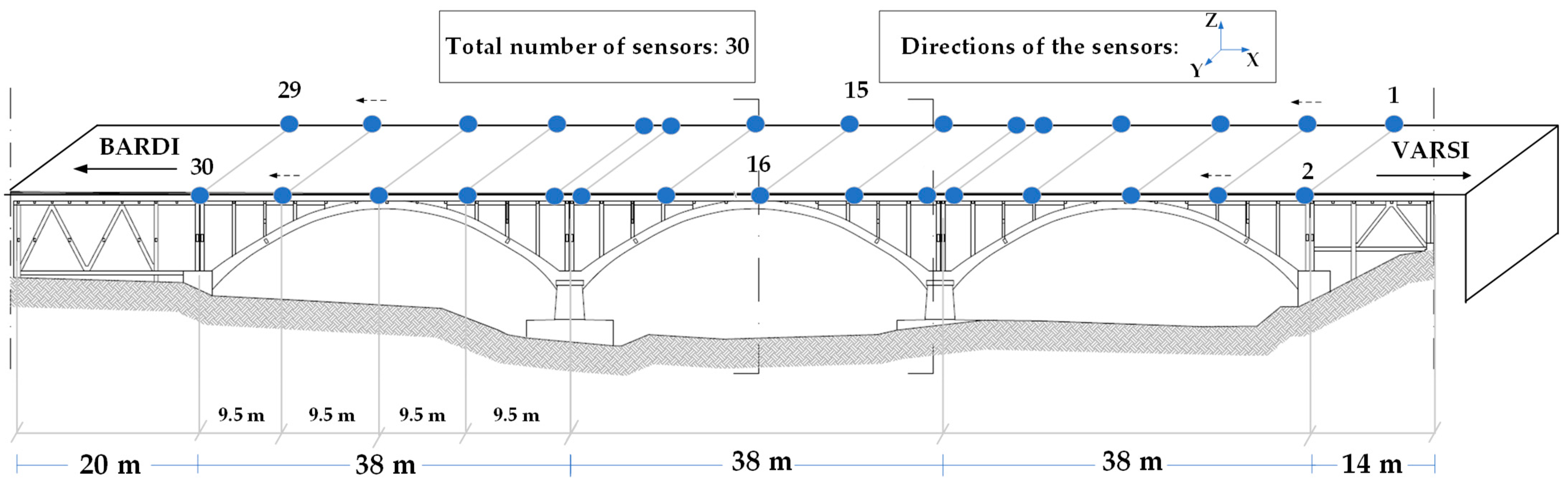
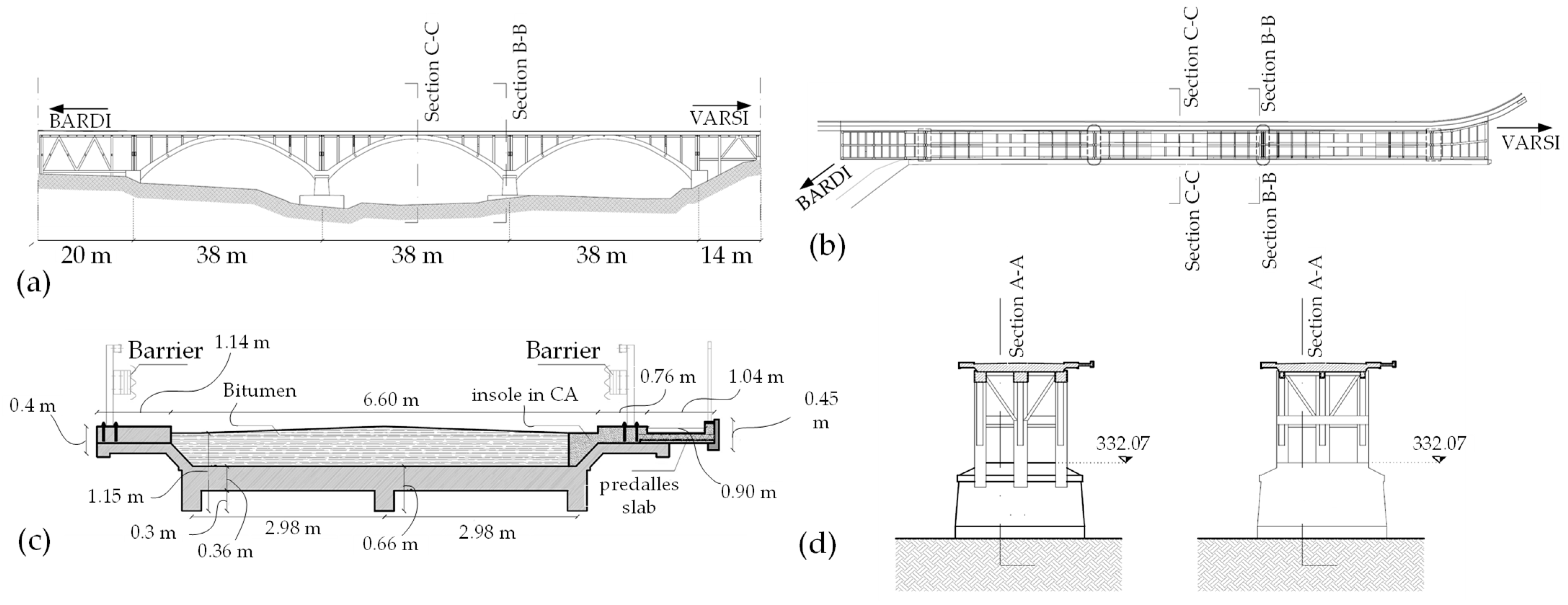
4.4.1. Bridge Description
4.4.2. Data Acquisition
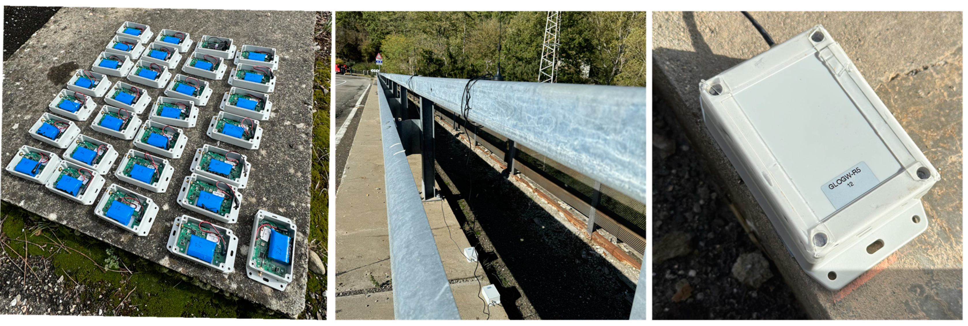
System Setup
System Configuration
Challenges
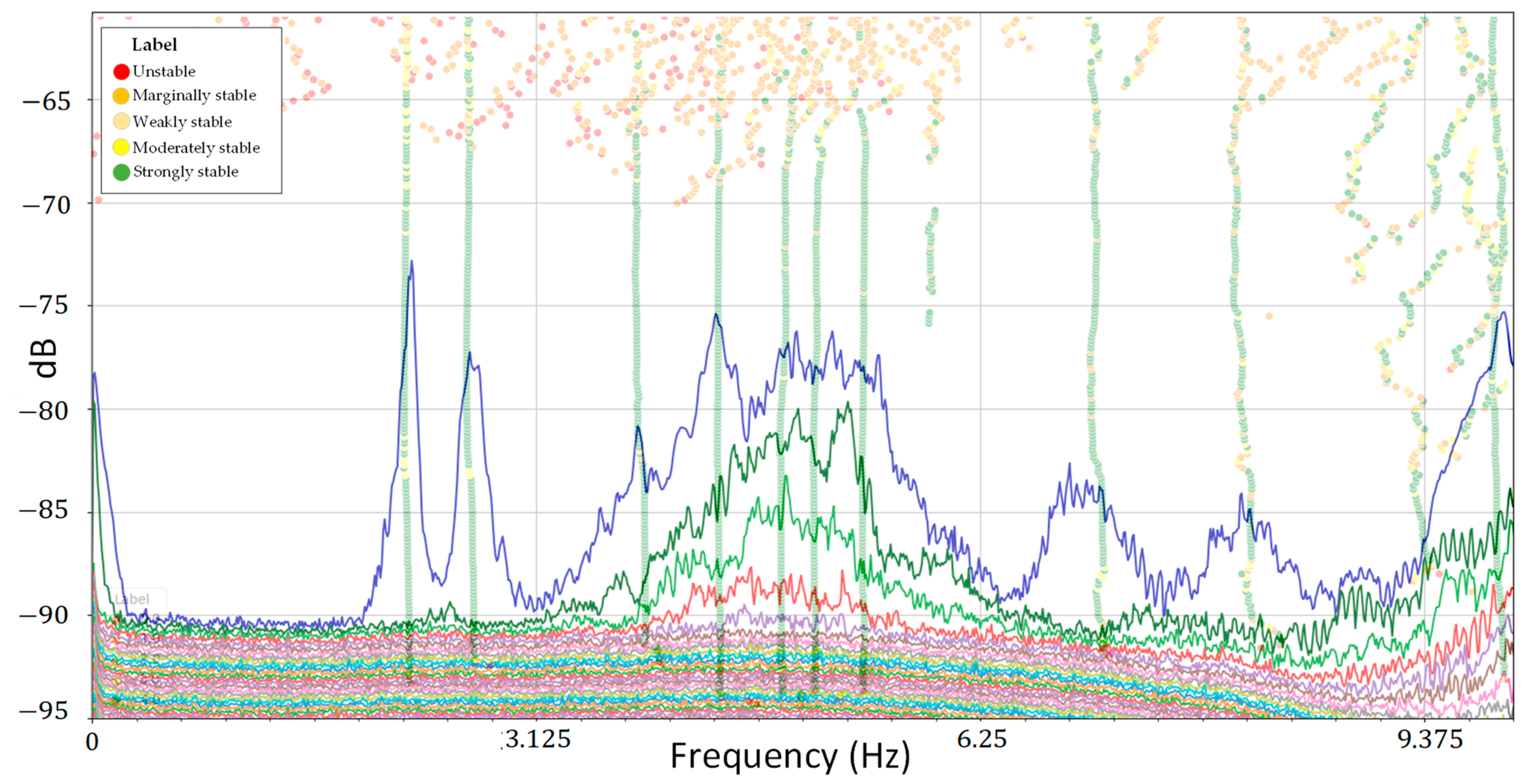
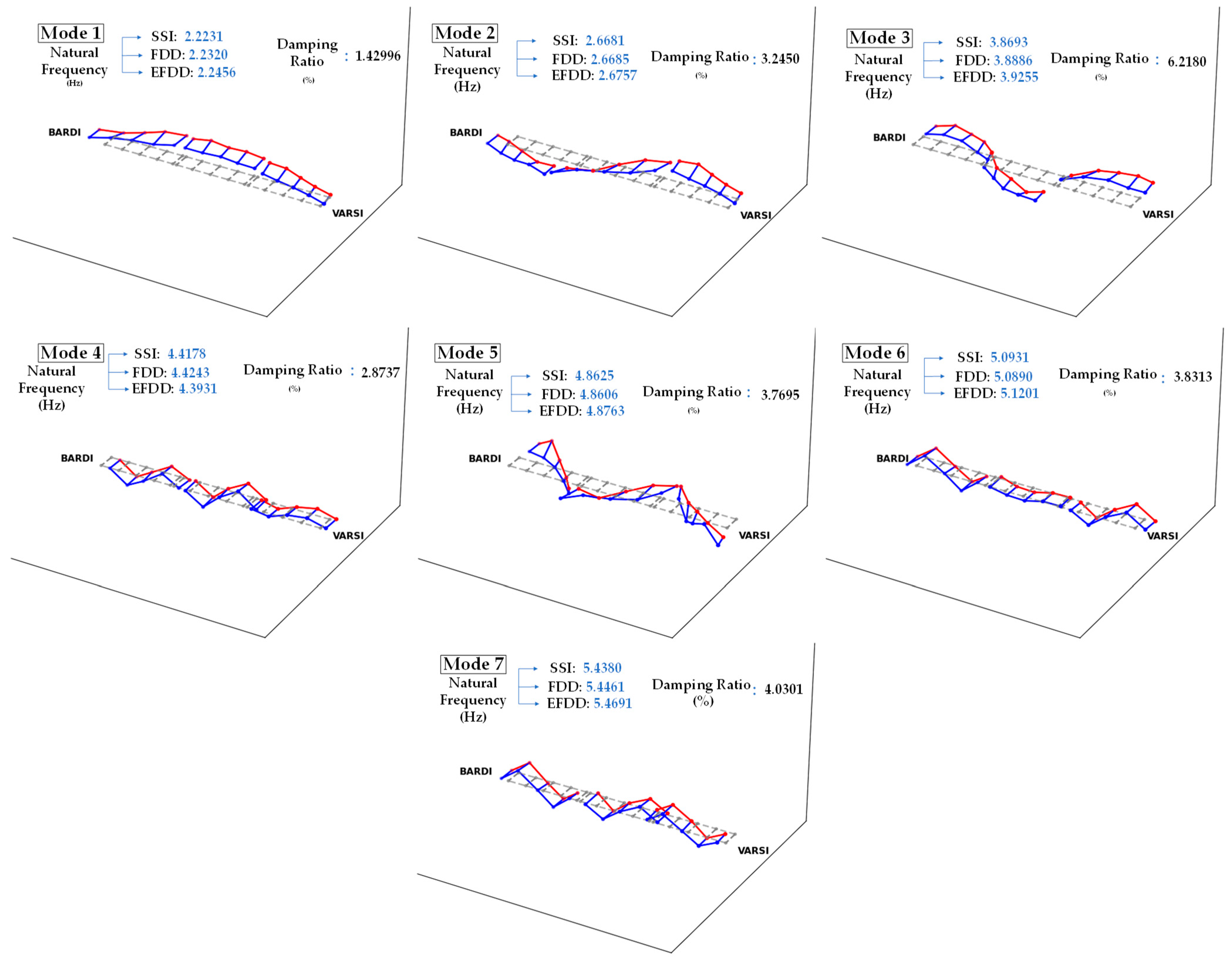
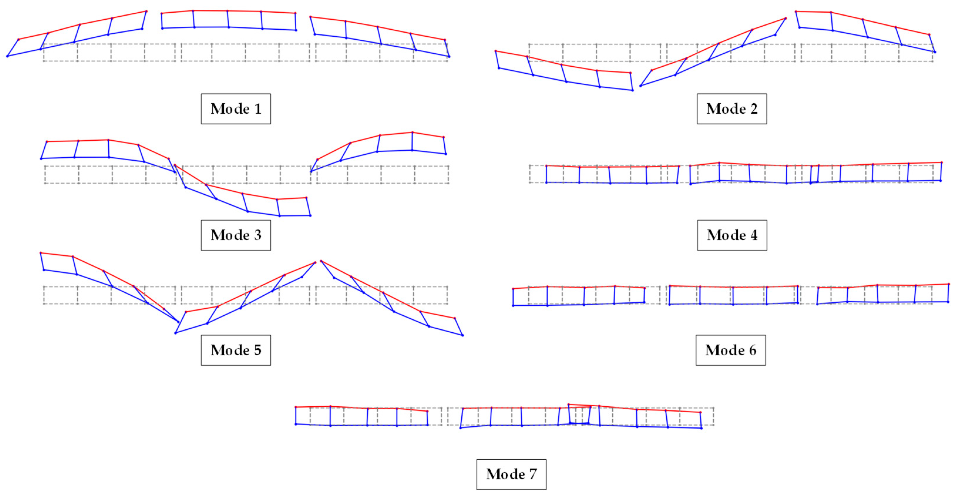
4.4.3. Operational Modal Analysis
Pre-Processing Step
Modal Identification Methods
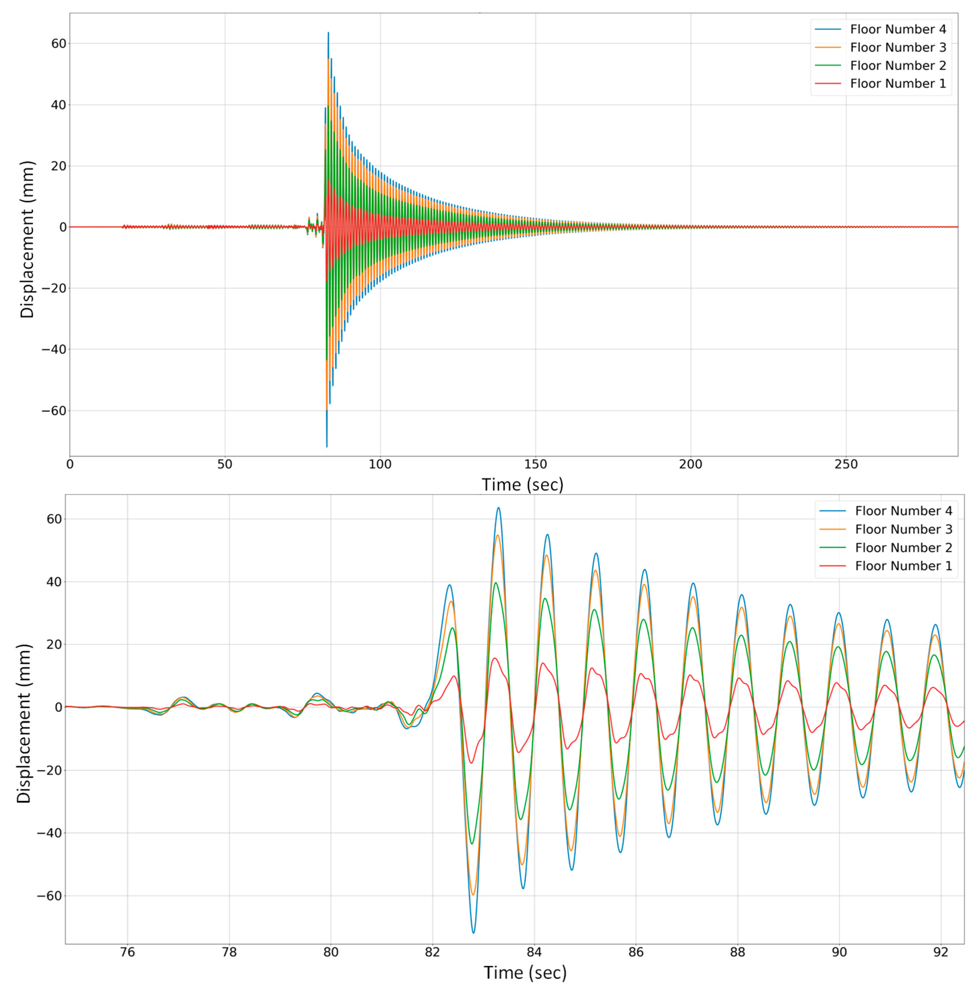
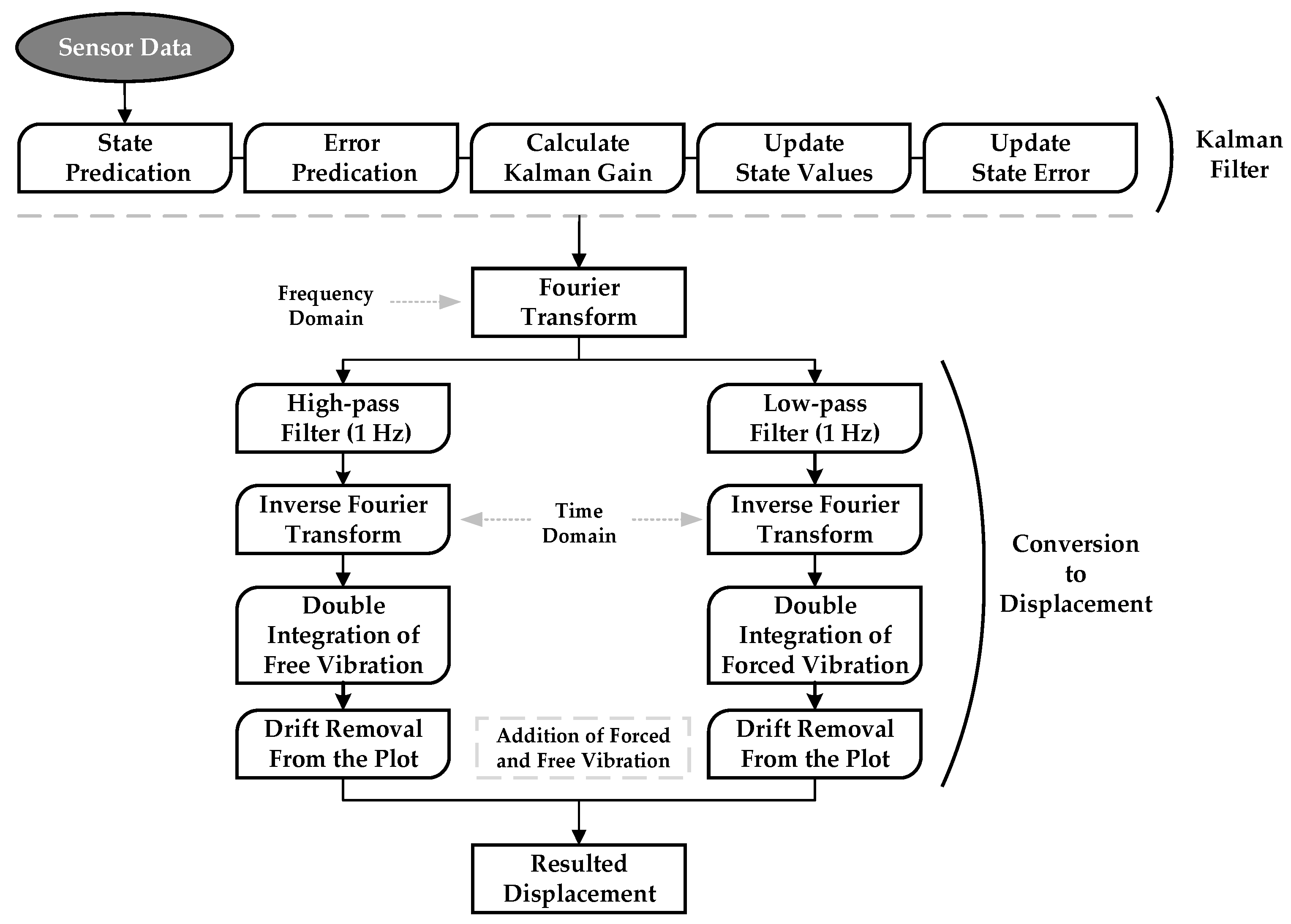
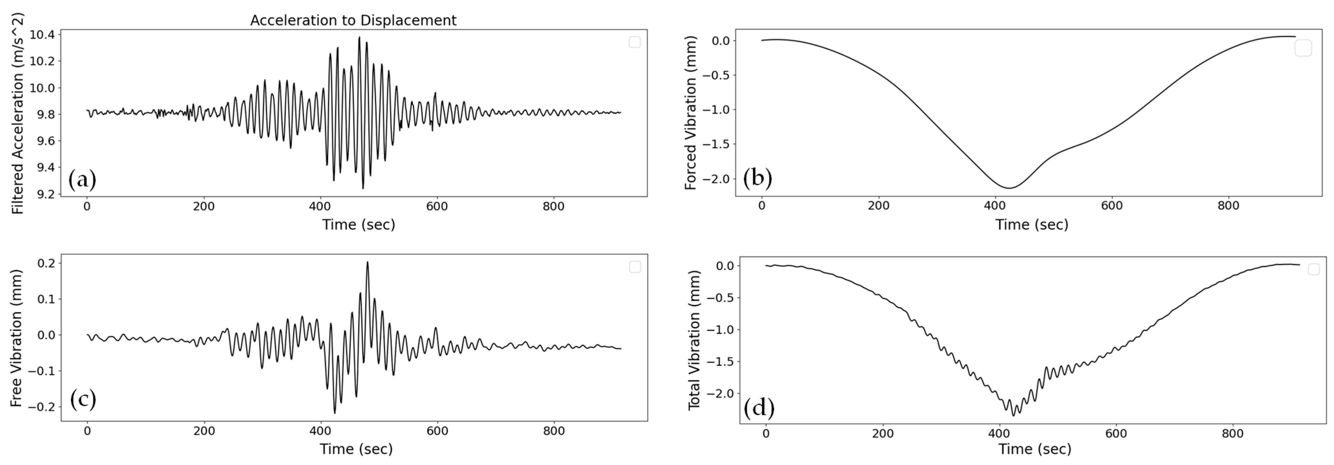
4.4.4. Displacement Calculation, Using Acceleration Data
5. Conclusions
Author Contributions
Funding
Institutional Review Board Statement
Informed Consent Statement
Data Availability Statement
Conflicts of Interest
References
- Chupanit, P.; Phromsorn, C. The Importance of Bridge Health Monitoring. World Acad. Sci. Eng. Technol. Int. J. Civ. Environ. Eng. 2012, 6, 135–138. [Google Scholar]
- Rashidi, M.; Mohammadi, M.; Sadeghlou Kivi, S.; Abdolvand, M.M.; Truong-Hong, L.; Samali, B. A Decade of Modern Bridge Monitoring Using Terrestrial Laser Scanning: Review and Future Directions. Remote Sens. 2020, 12, 3796. [Google Scholar] [CrossRef]
- Brincker, R.; Carlos, E. Ventura Introduction to Operational Modal Analysis; John Wiley & Sons: Hoboken, NJ, USA, 2015. [Google Scholar]
- Hasani, H.; Freddi, F. Operational Modal Analysis on Bridges: A Comprehensive Review. Infrastructures 2023, 8, 172. [Google Scholar] [CrossRef]
- Deng, Y.; Zhao, Y.; Ju, H.; Yi, T.-H.; Li, A. Abnormal Data Detection for Structural Health Monitoring: State-of-the-Art Review. Dev. Built Environ. 2024, 17, 100337. [Google Scholar] [CrossRef]
- Teixeira de Freitas, S.; Kolstein, H.; Bijlaard, F. Structural Monitoring of a Strengthened Orthotropic Steel Bridge Deck Using Strain Data. Struct. Health Monit. 2012, 11, 558–576. [Google Scholar] [CrossRef]
- Vicente, M.; Gonzalez, D.; Minguez, J.; Schumacher, T. A Novel Laser and Video-Based Displacement Transducer to Monitor Bridge Deflections. Sensors 2018, 18, 970. [Google Scholar] [CrossRef] [PubMed]
- Huber, M.S.; Bay, J.A.; Halling, M.W.; Womack, K.C. Use of Velocity Transducers in Low-Frequency Modal Testing of Structures. In Nondestructive Evaluation of Highways, Utilities, and Pipelines IV; SPIE: Bellingham, WA, USA, 2000; Volume 3995, pp. 414–424. [Google Scholar] [CrossRef]
- Ragam, P.; Sahebraoji, N.D. Application of MEMS-Based Accelerometer Wireless Sensor Systems for Monitoring of Blast-Induced Ground Vibration and Structural Health: A Review. IET Wirel. Sens. Syst. 2019, 9, 103–109. [Google Scholar] [CrossRef]
- Ghemari, Z. Study and Analysis of the Piezoresistive Accelerometer Stability and Improvement of Their Performances. Int. J. Syst. Assur. Eng. Manag. 2017, 8, 1520–1526. [Google Scholar] [CrossRef]
- Chen, Y.; Xue, X. Advances in the Structural Health Monitoring of Bridges Using Piezoelectric Transducers. Sensors 2018, 18, 4312. [Google Scholar] [CrossRef]
- Bedon, C.; Bergamo, E.; Izzi, M.; Noè, S. Prototyping and Validation of MEMS Accelerometers for Structural Health Monitoring—The Case Study of the Pietratagliata Cable-Stayed Bridge. J. Sens. Actuator Netw. 2018, 7, 30. [Google Scholar] [CrossRef]
- Sabato, A. Pedestrian Bridge Vibration Monitoring Using a Wireless MEMS Accelerometer Board. In Proceedings of the 2015 IEEE 19th International Conference on Computer Supported Cooperative Work in Design (CSCWD), Calabria, Italy, 6–8 May 2015; IEEE: New York, NY, USA, 2015; pp. 437–442. [Google Scholar]
- Bayraktar, A.; Altunişik, A.C.; Türker, T. Structural Condition Assessment of Birecik Highway Bridge Using Operational Modal Analysis. Int. J. Civ. Eng. 2016, 14, 35–46. [Google Scholar] [CrossRef]
- Zhang, G.; Moutinho, C.; Magalhães, F. Continuous Dynamic Monitoring of a Large-span Arch Bridge with Wireless Nodes Based on MEMS Accelerometers. Struct. Control Health Monit. 2022, 29, e2963. [Google Scholar] [CrossRef]
- Rainieri, C.; Fabbrocino, G. Operational Modal Analysis of Civil Engineering Structures: An Introduction and Guide for Applications; Springer: New York, NY, USA, 2014; ISBN 1493907670. [Google Scholar]
- Römer, K.; Blum, P.; Meier, L. Time Synchronization and Calibration in Wireless Sensor Networks. In Handbook of Sensor Networks: Algorithms and Architectures; John Wiley & Sons: Hoboken, NJ, USA, 2005; pp. 199–237. [Google Scholar] [CrossRef]
- Guerineau, L.; Mathé, L.; Le Roy, A. Development of an Integrated SHM Framework Based on a Novel Wireless Sensing System for Dynamic Structural Monitoring of Bridges Using Ambient Vibrations. In Proceedings of the 10th International Conference on Structural Health Monitoring of Intelligent Infrastructure, SHMII 10, Porto, Portugal, 30 June–2 July 2021. [Google Scholar]
- Araujo, A.; Garcia-Palacios, J.; Blesa, J.; Tirado, F.; Romero, E.; Samartin, A.; Nieto-Taladriz, O. Wireless Measurement System for Structural Health Monitoring With High Time-Synchronization Accuracy. IEEE Trans. Instrum. Meas. 2012, 61, 801–810. [Google Scholar] [CrossRef]
- He, L.; Reynders, E.; García-Palacios, J.H.; Carlo Marano, G.; Briseghella, B.; De Roeck, G. Wireless-Based Identification and Model Updating of a Skewed Highway Bridge for Structural Health Monitoring. Appl. Sci. 2020, 10, 2347. [Google Scholar] [CrossRef]
- Hu, X.; Wang, B.; Ji, H. A Wireless Sensor Network-Based Structural Health Monitoring System for Highway Bridges. Comput.-Aided Civ. Infrastruct. Eng. 2013, 28, 193–209. [Google Scholar] [CrossRef]
- Whelan, M.J.; Gangone, M.V.; Janoyan, K.D. Highway Bridge Assessment Using an Adaptive Real-Time Wireless Sensor Network. IEEE Sens. J. 2009, 9, 1405–1413. [Google Scholar] [CrossRef]
- Komarizadehasl, S.; Lozano, F.; Lozano-Galant, J.A.; Ramos, G.; Turmo, J. Low-Cost Wireless Structural Health Monitoring of Bridges. Sensors 2022, 22, 5725. [Google Scholar] [CrossRef]
- Abdulkarem, M.; Samsudin, K.; Rokhani, F.Z.; A Rasid, M.F. Wireless Sensor Network for Structural Health Monitoring: A Contemporary Review of Technologies, Challenges, and Future Direction. Struct. Health Monit. 2020, 19, 693–735. [Google Scholar] [CrossRef]
- Zhou, G.-D.; Yi, T.-H. Recent Developments on Wireless Sensor Networks Technology for Bridge Health Monitoring. Math. Probl. Eng. 2013, 2013, 947867. [Google Scholar] [CrossRef]
- Lynch, P. An Overview of Wireless Structural Health Monitoring for Civil Structures. Philos. Trans. R. Soc. Lond. Ser. A Math. Phys. Sci. 2005, 365, 345–372. [Google Scholar] [CrossRef] [PubMed]
- Sabato, A.; Niezrecki, C.; Fortino, G. Wireless MEMS-Based Accelerometer Sensor Boards for Structural Vibration Monitoring: A Review. IEEE Sens. J. 2017, 17, 226–235. [Google Scholar] [CrossRef]
- Kim, J.; Lynch, J.P.; Zonta, D.; Lee, J.-J.; Yun, C.-B. Reconfigurable Wireless Monitoring Systems for Bridges: Validation on the Yeondae Bridge. Proc. SPIE 2009, 7292, 72920T. [Google Scholar]
- Lynch, J.P.; Wang, Y.; Loh, K.J.; Yi, J.-H.; Yun, C.-B. Performance Monitoring of the Geumdang Bridge Using a Dense Network of High-Resolution Wireless Sensors. Smart Mater. Struct. 2006, 15, 1561–1575. [Google Scholar] [CrossRef]
- Dai, Z.; Wang, S.; Yan, Z. BSHM-WSN: A Wireless Sensor Network for Bridge Structure Health Monitoring. In Proceedings of the International Conference on Modelling, Identification and Control, Wuhan, China, 24–26 June 2012. [Google Scholar]
- Reyer, M.; Hurlebaus, S.; Mander, J.; Ozbulut, O.E. Design of a Wireless Sensor Network for Structural Health Monitoring of Bridges. In Proceedings of the 2011 Fifth International Conference on Sensing Technology, Palmerston North, New Zealand, 28 November–1 December 2011; IEEE: New York, NY, USA, 2011; pp. 515–520. [Google Scholar]
- Gutierrez, M.; Garita, C. Prototype Development of a Wireless Embedded System for Bridge Monitoring. In Proceedings of the 2017 IEEE 37th Central America and Panama Convention (CONCAPAN XXXVII), Managua, Nicaragua, 15–17 November 2017; IEEE: New York, NY, USA, 2017; pp. 1–6. [Google Scholar]
- Asadollahi, P.; Li, J. Statistical Analysis of Modal Properties of a Cable-Stayed Bridge through Long-Term Wireless Structural Health Monitoring. J. Bridge Eng. 2017, 22, 04017051. [Google Scholar] [CrossRef]
- Chae, M.J.; Yoo, H.S.; Kim, J.Y.; Cho, M.Y. Development of a Wireless Sensor Network System for Suspension Bridge Health Monitoring. Autom. Constr. 2012, 21, 237–252. [Google Scholar] [CrossRef]
- Sekiya, H.; Kimura, K.; Miki, C. Technique for Determining Bridge Displacement Response Using MEMS Accelerometers. Sensors 2016, 16, 257. [Google Scholar] [CrossRef]
- UNI 10985 2002; Vibrations on Bridges and Viaducts—Guidelines for Dynamic Tests and Surveys. UNI: Rome, Italy, 2002.
- Low Noise, Low Drift, Low Power, 3-Axis MEMS Accelerometers—ADXL354/ADXL355 (Rev. B); Analog Devices, Inc.: Norwood, MA, USA, 2016.
- Chen, Y.; Zheng, X.; Luo, Y.; Shen, Y.; Xue, Y.; Fu, W. An Approach for Time Synchronization of Wireless Accelerometer Sensors Using Frequency-Squeezing-Based Operational Modal Analysis. Sensors 2022, 22, 4784. [Google Scholar] [CrossRef]
- Noise and Vibration Seventh Edition—Measurement Handbook; Prosig: Fareham, UK, 2023.
- Lee, H.S.; Hong, Y.H.; Park, H.W. Design of an FIR Filter for the Displacement Reconstruction Using Measured Acceleration in Low-Frequency Dominant Structures. Int. J. Numer. Methods Eng. 2010, 82, 403–434. [Google Scholar] [CrossRef]
- Park, S.-K.; Park, H.W.; Shin, S.; Lee, H.S. Detection of Abrupt Structural Damage Induced by an Earthquake Using a Moving Time Window Technique. Comput. Struct. 2008, 86, 1253–1265. [Google Scholar] [CrossRef]
- Rollo, S. Caratterizzazione dinamica di ponti ad arco in cemento armato: Sperimentazione del ponte lamberti sul fiume ceno; Politecnico di Torino: Turin, Italy, 2018. [Google Scholar]
- Nhung, N.T.C.; Van Vu, L.; Nguyen, H.Q.; Huyen, D.T.; Nguyen, D.B.; Quang, M.T. Development and Application of Linear Variable Differential Transformer (LVDT) Sensors for the Structural Health Monitoring of an Urban Railway Bridge in Vietnam. Eng. Technol. Appl. Sci. Res. 2023, 13, 11622–11627. [Google Scholar] [CrossRef]
- Nassif, H.H.; Gindy, M.; Davis, J. Comparison of Laser Doppler Vibrometer with Contact Sensors for Monitoring Bridge Deflection and Vibration. NDT E Int. 2005, 38, 213–218. [Google Scholar] [CrossRef]
- Yoneyama, S.; Kitagawa, A.; Iwata, S.; Tani, K.; Kikuta, H. Bridge Deflection Measurement Using Digital Image Correlation. Exp. Tech. 2007, 31, 34–40. [Google Scholar] [CrossRef]
- Feng, D.; Feng, M.; Ozer, E.; Fukuda, Y. A Vision-Based Sensor for Noncontact Structural Displacement Measurement. Sensors 2015, 15, 16557–16575. [Google Scholar] [CrossRef]
- Busca, G.; Cigada, A.; Mazzoleni, P.; Zappa, E. Vibration Monitoring of Multiple Bridge Points by Means of a Unique Vision-Based Measuring System. Exp. Mech. 2014, 54, 255–271. [Google Scholar] [CrossRef]
- Helmi, K.; Taylor, T.; Zarafshan, A.; Ansari, F. Reference Free Method for Real Time Monitoring of Bridge Deflections. Eng. Struct. 2015, 103, 116–124. [Google Scholar] [CrossRef]
- Park, J.-W.; Sim, S.-H.; Jung, H.-J. Wireless Displacement Sensing System for Bridges Using Multi-Sensor Fusion. Smart Mater. Struct. 2014, 23, 045022. [Google Scholar] [CrossRef]
- Cho, S.; Sim, S.-H.; Park, J.-W.; Lee, J. Extension of Indirect Displacement Estimation Method Using Acceleration and Strain to Various Types of Beam Structures. Smart Struct. Syst. 2014, 14, 699–718. [Google Scholar] [CrossRef]
- Alfian, R.I.; Ma’arif, A.; Sunardi, S. Noise Reduction in the Accelerometer and Gyroscope Sensor with the Kalman Filter Algorithm. J. Robot. Control (JRC) 2021, 2, 180–189. [Google Scholar] [CrossRef]


| Attribute | Testing Conditions/Remarks | Average Value | Measurement Unit |
|---|---|---|---|
| Sensitivity | 2 g (X, Y, and Z) | 256,000 | LSB/g |
| Noise (spectral density) | 2 g (X, Y, and Z) | 22.5 | |
| Sensitivity change due to temperature | 0.01 | ||
| Nonlinearity | 2 g | 0.1 | |
| Zero offset | 2 g (X, Y, and Z) | 25 | mg |
| Stages | Power Consumption | Time Per Day |
|---|---|---|
| Transmission | 125 mA | 20 s |
| Sampling | 3 mA | 30 min |
| Stand-by | 5.5 uA | 24 h |
| Noise Axis | Peak to Peak (mg) | RMS Noise (mg) | Noise Density ) |
|---|---|---|---|
| X | 0.6899 | 0.0891 | 17.79 |
| Y | 1.0250 | 0.0909 | 19.57 |
| Z | 1.0173 | 0.1191 | 22.49 |
| Average | 0.9108 | 0.0997 | 19.95 |
| Modes | Natural Frequency (Hz) | Relative Difference (%) | Damping Ratio (%) | ||||||
|---|---|---|---|---|---|---|---|---|---|
| PP | FDD | SSI | FEM | PP vs. SSI | FDD vs. SSI | FEM vs. FDD | FEM vs. SSI | SSI | |
| First | 2.03 | 2.03 | 2.03 | 2.07 | <0.01 | <0.01 | 1.98 | 2.01 | 1.08 |
| Second | 6.15 | 6.15 | 6.14 | 6.14 | 0.16 | 0.32 | 0.02 | 0.04 | 0.28 |
| Third | 9.81 | 9.8 | 9.81 | 9.96 | <0.01 | 0.2 | 1.52 | 2.61 | 0.35 |
| Fourth | 12.15 | 12.15 | 12.18 | 12.69 | 0.25 | 0.48 | 4.1 | 6.07 | 0.53 |
| Modes | Type | Natural Frequency (Hz) | Relative Difference (%) | Damping (%) | |||||
|---|---|---|---|---|---|---|---|---|---|
| PP | FDD | EFDD | SSI_Cov | FDD vs. EFDD | FDD vs. SSI_Cov | EFDD vs. SSI_Cov | SSI | ||
| First | First transverse | 2.2 | 2.23 | 2.25 | 2.22 | −0.89 | 0.4 | 1 | 1.43 |
| Second | Second transverse | 2.7 | 2.67 | 2.68 | 2.67 | −0.27 | 0.01 | 0.28 | 3.24 |
| Third | Third transverse | 3.9 | 3.89 | 3.93 | 3.87 | −0.95 | 0.5 | 1.43 | 6.22 |
| Fourth | First vertical | 4.4 | 4.42 | 4.39 | 4.42 | 0.71 | 0.15 | −0.56 | 2.87 |
| Fifth | First torsion | 4.9 | 4.86 | 4.88 | 4.86 | −0.32 | −0.04 | 0.28 | 3.77 |
| Sixth | Second vertical | 5.1 | 5.09 | 5.12 | 5.09 | −0.61 | −0.08 | 0.53 | 3.83 |
| Seventh | Third vertical | 5.4 | 5.45 | 5.47 | 5.44 | −0.42 | 0.15 | 0.57 | 4.03 |
| Modes | Natural Frequency (Hz) | Relative Difference (%) | ||||
|---|---|---|---|---|---|---|
| Thesis [42] | EFDD | SSI-Cov | Thesis vs. EFDD | Thesis vs. SSI-Cov | Average | |
| First | 2.29 | 2.25 | 2.22 | −1.75 | −3.11 | −2.43 |
| Second | 3.10 | 2.68 | 2.67 | −13.55 | −16.04 | −14.80 |
| Third | 4.22 | 3.93 | 3.87 | −6.87 | −8.91 | −7.89 |
Disclaimer/Publisher’s Note: The statements, opinions and data contained in all publications are solely those of the individual author(s) and contributor(s) and not of MDPI and/or the editor(s). MDPI and/or the editor(s) disclaim responsibility for any injury to people or property resulting from any ideas, methods, instructions or products referred to in the content. |
© 2024 by the authors. Licensee MDPI, Basel, Switzerland. This article is an open access article distributed under the terms and conditions of the Creative Commons Attribution (CC BY) license (https://creativecommons.org/licenses/by/4.0/).
Share and Cite
Hasani, H.; Freddi, F.; Piazza, R.; Ceruffi, F. A Wireless Data Acquisition System Based on MEMS Accelerometers for Operational Modal Analysis of Bridges. Sensors 2024, 24, 2121. https://doi.org/10.3390/s24072121
Hasani H, Freddi F, Piazza R, Ceruffi F. A Wireless Data Acquisition System Based on MEMS Accelerometers for Operational Modal Analysis of Bridges. Sensors. 2024; 24(7):2121. https://doi.org/10.3390/s24072121
Chicago/Turabian StyleHasani, Hamed, Francesco Freddi, Riccardo Piazza, and Fabio Ceruffi. 2024. "A Wireless Data Acquisition System Based on MEMS Accelerometers for Operational Modal Analysis of Bridges" Sensors 24, no. 7: 2121. https://doi.org/10.3390/s24072121
APA StyleHasani, H., Freddi, F., Piazza, R., & Ceruffi, F. (2024). A Wireless Data Acquisition System Based on MEMS Accelerometers for Operational Modal Analysis of Bridges. Sensors, 24(7), 2121. https://doi.org/10.3390/s24072121