Article

An Improved Theory for Designing and Numerically Calibrating Circular Touch Mode Capacitive Pressure Sensors

1
School of Civil Engineering, Chongqing University, Chongqing 400045, China
2
Key Laboratory of New Technology for Construction of Cities in Mountain Area (Chongqing University), Ministry of Education, Chongqing 400045, China
*
Author to whom correspondence should be addressed.
Sensors 2024, 24(3), 907; https://doi.org/10.3390/s24030907
Submission received: 13 December 2023 / Revised: 22 January 2024 / Accepted: 29 January 2024 / Published: 30 January 2024
(This article belongs to the Collection Instrument and Measurement)

Abstract

:
The design, especially the numerical calibration, of a circular touch mode capacitive pressure sensor is highly dependent on the accuracy of the analytical solution of the contact problem between the circular conductive membrane and the rigid plate of the sensor. In this paper, the plate/membrane contact problem is reformulated using a more accurate in-plane equilibrium equation, and a new and more accurate analytical solution is presented. On this basis, the design and numerical calibration theory for circular touch mode capacitive pressure sensors has been greatly improved and perfected. The analytical relationships of pressure and capacitance are numerically calculated using the new and previous analytical solutions, and the gradually increasing difference between the two numerical calculation results with the gradual increase in the applied pressure is graphically shown. How to use analytical solutions and analytical relationships to design and numerically calibrate a circular touch mode capacitive pressure sensor with a specified pressure detecting range is illustrated in detail. The effect of changing design parameters on capacitance–pressure analytical relationships is comprehensively investigated; thus, the direction of changing design parameters to meet the required or desired range of pressure or capacitance is clarified.

1. Introduction

Membranes have a wide range of applications in engineering, technology and other fields, such as space engineering [1], wastewater treatment [2], bionic structure of tympanic membranes [3] and so on. Many membranes have the ability to exhibit large elastic deflections under transverse loading [4,5,6,7,8,9,10], which provides the possibility of designing and developing deflection-based devices [11,12,13,14,15,16,17,18,19]. For instance, the circular capacitive pressure sensor addressed here is such a deflection-based device, which is a pressure sensor using a circular conductive membrane as the sensitive element and a variable capacitor as the sensing element. The circular conductive membrane, which works as the movable electrode plate of the variable capacitor, elastically deflects toward the fixed electrode plate of the variable capacitor under pressure, resulting in the capacitance change in the variable capacitor. So, the testing principle of such a capacitive pressure sensor is to detect the applied pressure by measuring the capacitance change under the applied pressure, where the sensitive element (the circular conductive membrane) converts the pressure to be detected to the membrane deflection, and the sensing element (the variable capacitor) converts the membrane deflection to the capacitance. Such sensors usually operate in non-touch (or normal) mode or touch mode, and can be embedded or packaged for use, for example, embedded in industrial structures such as tires, or packaged as conventional sensors for industrial field applications. Considering that the touch mode of operation has many advantages over the non-touch mode of operation, this paper is devoted to the improvement of the design and numerical calibration theory for circular touch mode capacitive pressure sensors.
The key element of a circular capacitive pressure sensor is a circular variable capacitor using a circular conductive membrane and a thin plate as the movable and fixed electrode plates, as shown in Figure 1, where a is the radius of the initially flat circular conductive membrane; g is the initially parallel gap between the initially flat circular conductive membrane and the insulator layer; t is the thickness of the insulator layer; the dash–dotted line represents the geometric middle plane of the initially flat circular conductive membrane; q is the pressure to be detected; q TPP is the touch point pressure when the circular conductive membrane under the pressure q just touches the insulator layer; b is the radius of the circular contact area between the deflected conductive membrane and the insulator layer; o denotes the origin of the introduced cylindrical coordinate system (r, φ, w); r is the radial coordinate; φ is the angle coordinate but is not represented due to the characteristics of axial symmetry and w is the transverse coordinate that also denotes the deflection in the circular conductive membrane under the pressure q.
Before application of the pressure q, as shown in Figure 1a, the circular conductive membrane is initially flat (undeflected), the circular conductive thin plate is fixed on the substrate and coated with a thin layer of insulator and the initially parallel gap between the initially flat circular conductive membrane and the insulator layer is filled with air. On application of the pressure q, as shown in Figure 1b, the initially flat circular conductive membrane elastically deflects towards the insulator layer and is thus known as a movable electrode plate, while the circular conductive thin plate fixed on the substrate is known as a fixed electrode plate. When the pressure q reaches the touch point pressure q TPP , the deflected conductive membrane just touches the insulator layer, as shown in Figure 1c.
Therefore, before the pressure q reaches the touch point pressure q TPP , the total capacitor between the movable and fixed electrode plates can be regarded as one consisting of two capacitors in series. The first capacitor is the one between the conductive membrane and the insulator layer, and the second capacitor is the one between the insulator layer and the conductive thin plate. Obviously, the application of the pressure q only causes a change in the capacitance of the first capacitor and does not affect the capacitance of the second capacitor. So, the first capacitor is known as a variable capacitor and the second capacitor is known as a fixed capacitor. The first capacitor changes from the parallel plate capacitor before application of the pressure q to the non-parallel plate capacitor after application of the pressure q (from the initially parallel gap g to the non-parallel gap gw(r), see Figure 1a,b), and the second capacitor always remains as a parallel plate capacitor (whose parallel gap is the thickness t of the insulator layer). Of course, the total capacitor between the movable and fixed electrode plates is also a variable capacitor.
After the pressure q exceeds the touch point pressure q TPP , that is, when q > q TPP , a circular contact area will be formed between the deflected conductive membrane and the insulator layer, and the radius b of the circular contact area will gradually increase as the pressure q further increases, as shown in Figure 1d. At this time, the total capacitor between the movable and fixed electrode plates (which will be denoted by C in Section 3) can be regarded as one consisting of two capacitors in parallel (which will be denoted by C1 and C2 in Section 3). C1 refers to the parallel plate capacitor in the contact area of 0rb (the parallel gap between its two electrode plates is equal to the thickness t of the insulator layer, see Figure 1d), and is a variable capacitor due to the gradually increasing b. C2 refers to the non-parallel plate capacitor in the non-contact area of bra, and can be regarded as one consisting of two capacitors in series (which will be denoted by C3 and C4 in Section 3). C3 refers to the parallel plate capacitor in the non-contact area of bra (the parallel gap between its two electrode plates is equal to the thickness t of the insulator layer, see Figure 1d) and is a variable capacitor due to the gradually increasing b. C4 refers to the non-parallel plate capacitor in the non-contact area of bra (the non-parallel gap between its two electrode plates is equal to g–w(r), see Figure 1d) and is also a variable capacitor due to the gradually increasing b as well as the non-parallel gap g–w(r) varying with the applied pressure q.
The circular capacitive pressure sensor in Figure 1 is said to operate in touch mode when q > q TPP , to operate in non-touch (or normal) mode when q < q TPP , to be in a critical state when q   = q TPP , and to be in an initial state when q   = 0 , corresponding to Figure 1a–d, respectively.
Capacitive pressure sensors are less sensitive to side stress and other environmental effects, and have high sensitivity, robust structure and no turn-on temperature drift [20,21]. A capacitive pressure sensor is called a non-touch (or normal) mode capacitive pressure sensor if it operates in non-touch (or normal) mode, and is called a touch mode capacitive pressure sensor if it operates in touch mode. Obviously, since the substrate can directly bear the pressure q applied in the plate/membrane contact area of 0rb (see Figure 1d), the touch mode capacitive pressure sensor has larger overload protection, in comparison with the non-touch mode capacitive pressure sensor. This implies that the pressure range when a capacitive pressure sensor operates in touch mode is much wider than that when this capacitive pressure sensor operates in non-touch (or normal) mode. Therefore, the touch mode capacitive pressure sensors can show better performance, especially in industrial applications. In the specific design and fabrication of a capacitive pressure sensor, it is very important to accurately understand the stress, strain and displacement in the circular conductive membrane under the pressure q. Therefore, it is often necessary to analytically solve the elastic behavior of the circular conductive membrane under the pressure q.
On the other hand, it can be seen from Figure 1b,d that under the pressure q, the circular conductive membrane is in a state of free deflection when the sensor operates in non-touch (or normal) mode, and when the sensor operates in touch mode, it is in a state of limited maximum deflection. The former is a large deflection problem of a circular membrane under transverse uniform loading (the well-known Föppl–Hencky membrane problem), while the latter is an axisymmetric contact problem between a deflected circular membrane and a rigid plate (which is usually called the plate/membrane contact problem for short). In comparison with the analytical solution to the plate/membrane contact problem, the well-known Föppl–Hencky membrane problem is much easier to be analytically solved.
In fact, the Föppl–Hencky membrane problem has been very well solved analytically [22,23,24,25], but the analytical solution of the plate/membrane contact problem still needs to be further improved. Xu and Liechti solved this plate/membrane contact problem based on the assumptions of an equi-biaxial constant stress state and small rotation angle of the membrane [26]. Wang et al. presented a closed-form solution of this plate/membrane contact problem by giving up the assumption of equi-biaxial constant stress state for the first time [27]. Lian et al. also presented a closed-form solution of this plate/membrane contact problem [28], where the equi-biaxial constant stress state assumption was given up, and the out-of-plane equilibrium equation used was established by giving up the small rotation angle assumption of the membrane. Li et al. presented a more refined closed-form solution of this plate/membrane contact problem [29], where the out-of-plane equilibrium equation and geometric equations used were established by giving up the small rotation angle assumption of the membrane, except for giving up the equi-biaxial constant stress state assumption. However, the in-plane equilibrium equation used in [26,27,28,29] is the classic one, which does not take into account the contribution of deflection to in-plane equilibrium at all and is only applicable to plane-stretched or compressed membranes and not to large deflection membranes. In other words, the classic in-plane equilibrium equation used in [26,27,28,29] is only applicable to the plane-stretched membrane in the plate/membrane contact area of 0rb and not to the large deflection membrane in the plate/membrane non-contact area of bra (see Figure 1d). So, in [26,27,28,29], the use of the classic in-plane equilibrium equation inevitably introduces calculation errors. In this paper, the plate/membrane contact problem is reformulated using a more accurate in-plane equilibrium equation which fully takes into account the contribution of deflection to the in-plane equilibrium [25], resulting in a new and more accurate analytical solution of the problem. On this basis, the design and numerical calibration theory for circular touch mode capacitive pressure sensors have been greatly improved and perfected.
This paper is organized in the order of, first, the sensitive element, then the sensing element, then the results and discussion, and finally the concluding remarks. In the following section, depending on the magnitude of the applied pressure q (see Figure 1), the elastic behavior of the sensitive element (the circular conductive membrane) is reduced to a large deflection problem (Figure 1b) and a plate/membrane contact problem (Figure 1d), respectively. The new and more accurate analytical solution of the plate/membrane contact problem in Figure 1d is presented, where the stress solution is used for the strength design of the sensitive element, and the deflection solution is used for determining the total capacitance of the sensing element (the capacitor between the movable and fixed electrode plates, see Figure 1d). In Section 3, based on the newly presented deflection solution, the analytical relationship between the total capacitance and the applied pressure q is derived and discussed. In Section 4, an example is first given to illustrate how to use the analytical solutions of the large deflection problem and plate/membrane contact problem as well as the pressure–capacitance analytical relationship to design and numerically calibrate a circular touch mode capacitive pressure sensor with a specified pressure detecting range. Then, the analytical relationships of the capacitance as input and the applied pressure as output are calculated using the newly and previously presented analytical solutions, and are compared to show the rapidly increasing difference between the two calculated results with the increase in the applied pressure. Finally, the effect of changing design parameters on input capacitance–output pressure relationships is comprehensively investigated, including changing the radius a, thickness h, Poisson’s ratio v and Young’s modulus of elasticity E of the circular conductive membrane, as well as the thickness t of the insulator layer and the initially parallel gap g between the initially flat circular conductive membrane and the insulator layer. Concluding remarks are given in Section 5.
The contribution of this study mainly lies in the following two aspects. One is purely a mechanical contribution: using a more accurate in-plane equilibrium equation, a new and more accurate analytical solution of the plate/membrane contact problem is presented for the first time. The other aspect is the technical contribution: based on the newly presented analytical solution, the design and numerical calibration theory for circular touch mode capacitive pressure sensors has been greatly improved and perfected on the basis of the existing theory.

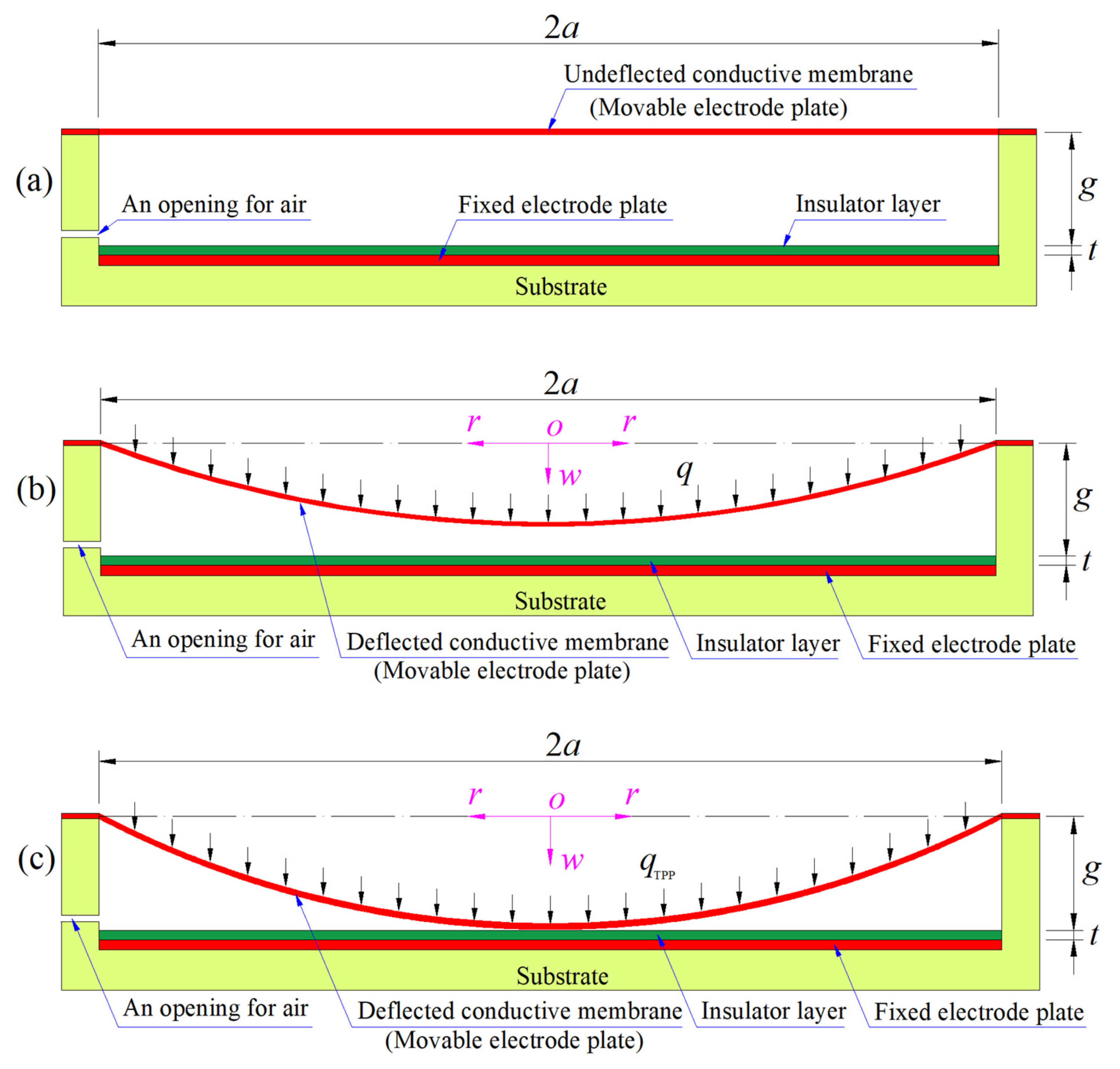
2. More Refined Analytical Solution to the Sensitive Element of the Sensor

The circular conductive membrane, as the sensitive element of the circular capacitive pressure sensor, produces axisymmetric deformation with a large deflection in response to the applied pressure q, as shown in Figure 1. Before the pressure q reaches the touch point pressure q TPP (see Figure 1c), the initially flat circular conductive membrane (see Figure 1a) is in a state of free deflection, as shown in Figure 1b, which is usually called the large deflection problem of circular membranes under uniformly distributed transverse loads. This large deflection problem of circular membranes was dealt with originally by Föppl [30] and Hencky [31], and is usually called the Föppl–Hencky membrane problem. After the pressure q reaches the touch point pressure q TPP , the deflected circular conductive membrane is in a state of limited maximum deflection, as shown in Figure 1d, which is known as an axisymmetric contact problem between a deflected circular membrane and a rigid plate, or the plate/membrane contact problem for short.
The plate/membrane contact problem has many potential applications such as the membrane/substrate delamination [32,33,34], adhesion [35,36,37,38,39,40] and especially capacitive pressure sensors [41,42,43,44,45,46,47,48,49,50,51]. However, the plate/membrane contact problem involves both the plane-stretched membrane in the plate/membrane contact area of 0rb and the large deflection membrane in the plate/membrane non-contact area of bra (see Figure 1d). But the existing analytical solutions of the plate/membrane contact problem [26,27,28,29] are all obtained using the classic in-plane equilibrium equation that is only applicable to the plane-stretched membrane problems, which inevitably introduces calculation errors. In this paper, this plate/membrane contact problem is further analytically solved by giving up the equi-biaxial constant stress state assumption and using more accurate out-of-plane and in-plane equilibrium equations and geometric equations, and a new and more refined closed-form solution is presented, which is detailed as follows.
Suppose that the circular conductive membrane in Figure 1 has Young’s modulus E, Poisson’s ratio ν, thickness h and radius a. After the pressure q reaches the touch point pressure q TPP , the circular conductive membrane comes into axisymmetric contact with the insulator layer, resulting in a contact radius b. The maximum deflection wm of the circular membrane is always equal to the initially parallel gap g, that is, w(r) ≡ g when rb (see Figure 1d). Throughout the following formulation, it is assumed that the circular membrane always has a constant thickness h during its deflection. In this plate/membrane axisymmetric contact problem, the whole deflected circular membrane may be divided into two parts: one is a circular plate/membrane contact area with a contact radius b and the other part is an annular plate/membrane non-contact area with an inner radius b and an outer radius a. In the plate/membrane contact area, the circular membrane only undergoes the in-plane axisymmetric stretching (only a plane problem), while in the plate/membrane non-contact area, the annular membrane undergoes the out-of-plane axisymmetric deflection. The stress, strain and displacement of the membrane should be continuous at the connecting ring between the annular region and the circular region, i.e., at r = b (see Figure 1d). Such a continuity condition will be used as conditions for determining special solutions.
A free body of radius r (bra) is assumed to be taken from the circular conductive membrane in contact with the insulator layer in Figure 1d, as shown in Figure 2, to study its static problem of equilibrium, where σr is the radial stress at r and θ is the meridional rotation angle of the deflected membrane at r.
In the vertical direction perpendicular to the initially flat circular membrane (represented by the dash–dotted line in Figure 2), the vertical forces are πr2q (the total force of the uniformly distributed transverse loads q within radius r), πb2q (the total reaction force from the rigid plate) and 2πrσrhsinθ (the total vertical force produced by the membrane force σrh), where bra. Therefore, the out-of-plane equilibrium equation can be derived from the condition that the resultant force should be equal to zero in the vertical direction, i.e.,
π r 2 q π b 2 q 2 π r σ r h sin θ = 0 ,
where
sin θ = 1 / 1 + 1 / tan 2 θ = 1 / 1 + 1 / ( d w / d r ) 2 .
Substituting Equation (2) into Equation (1) yields
( r 2 b 2 ) q 1 + 1 / ( d w / d r ) 2 = 2 r σ r h .
The classic in-plane equilibrium equation does not take into account the contribution of deflection to in-plane equilibrium at all [22,26,27,28,29,31]. So, Li et al. modified the classic in-plane equilibrium equation, but presented only an in-plane equilibrium equation partly taking into account the contribution of deflection to in-plane equilibrium [4]. The in-plane equilibrium equation that fully takes into account the contribution of deflection to in-plane equilibrium was established by Sun et al. [25], and is given by
d d r [ r σ r 1 + ( d w d r ) 2 ] σ t 1 + ( d w d r ) 2 = 0 ,
where σt denotes the circumferential stress.
Obviously, if the membrane is in the plane-stretched or compressed state, then the membrane is flat, the first derivative of the deflection w(r) is thus equal to zero, i.e., dw/dr ≡ 0. Therefore, after substituting dw/dr = 0 into Equation (4), we can obtain the classic in-plane equilibrium equation in [22,26,27,28,29,31], that is, d ( r σ r ) / d r σ t = 0 . So, the classic in-plane equilibrium equation used in [22,26,27,28,29,31] is only applicable to the membrane in the plate/membrane contact area of 0 ≤ rb, and not to the large deflection membrane in the plate/membrane non-contact area of bra (see Figure 2).
In order to take into account the effect of deflection on geometric relationship, the geometric equations (the relationships between strain and displacement) have been modified from the classic one [22,31] into the following form [24]
e r = [ ( 1 + d u d r ) 2 + ( d w d r ) 2 ] 1 / 2 1
and
e t = u r ,
where er, et and u denote the radial and circumferential strains and radial displacement, respectively. Moreover, the relationships between stress and strain are still assumed to be linearly elastic and given by the generalized Hooke’s law
σ r = E 1 ν 2 ( e r + ν e t )
and
σ t = E 1 ν 2 ( e t + ν e r ) .
Substituting Equations (5) and (6) into Equations (7) and (8) yields
σ r = E 1 ν 2 { [ ( 1 + d u d r ) 2 + ( d w d r ) 2 ] 1 / 2 1 + ν u r }
and
σ t = E 1 ν 2 { u r + ν [ ( 1 + d u d r ) 2 + ( d w d r ) 2 ] 1 / 2 ν } .
By means of Equations (4), (9) and (10), one has
u r = 1 E ( σ t ν σ r ) .
After substituting the u in Equation (11) into Equation (9), the consistency equation may be written as
( 1 E σ r + 1 ν E σ t ) 2 1 + d d r [ 1 E r ( σ t ν σ r ) ] 2 d w d r 2 = 0 .
Therefore, the radial and circumferential stresses σr and σt and the deflection w(r) within bra can be determined by simultaneously solving Equations (3), (4) and (12). The conditions for determining the special solutions of σr, σt and w(r) are the boundary conditions at r = a, as well as the continuity conditions at r = b, which can be determined only by solving the plane problem of axisymmetric stretching of the circular membrane in the plate/membrane contact area with radius 0 ≤ rb, which is detailed as follows.
Obviously, in the plate/membrane contact area with radius 0 ≤ rb, the membrane is flat, then the first derivative of the deflection w(r) is always zero, i.e., dw/dr ≡ 0 for 0 ≤ rb. Therefore, it can be obtained from Equations (5) and (6) that
e r = d u d r
and
e t = u r .
Substituting Equations (13) and (14) into Equations (7) and (8) yields
σ r = E 1 ν 2 ( d u d r + ν u r )
and
σ t = E 1 ν 2 ( u r + ν d u d r ) .
Substituting Equations (15) and (16) into Equation (4), one has
r d 2 u d r 2 + d u d r u r = 0 .
Since Equation (17) satisfies the form of the Euler equation, the general solution of Equation (17) can be written as
u ( r ) = K 1 r + K 2 r ,
where K1 and K2 are two unknown constants. It is not difficult to understand that since the radial displacement u is finite at r = 0, the unknown constant K2 has to be equal to zero. So, if the radial displacement u(r) at r = b is denoted by u(b), then K1 = u(b)/b. Therefore, the radial displacement may be written as
u ( r ) = u ( b ) b r .
Substituting Equation (19) into Equations (13)–(16) yields
e r = e t = u ( b ) b
and
σ r = σ t = E 1 ν u ( b ) b .
Equations (20) and (21) suggest that the strain and stress are uniformly distributed in the plate/membrane contact area with radius 0 ≤ rb.
Therefore, the boundary conditions at r = a are
w = 0   at   r = a
and
e t = 1 E ( σ t ν σ r ) = 0   at   r = a .
The continuity conditions at r = b are
w = g   at   r = b ,
( u r ) A = ( u r ) B = u ( b ) b   at   r = b
and
( σ r ) A = ( σ r ) B = E 1 ν u ( b ) b   at   r = b ,
where ( )A and ( )B represent the values of various variables on two sides of the interconnecting circle of r = b and the subscript A refers to the side of plate/membrane non-contact area of bra while the subscript B refers to the side of plate/membrane contact area of 0 ≤ rb.
Let us introduce the following dimensionless variables
Q = q a E h ,   W = w a ,   S r = σ r E ,   S t = σ t E ,   x = r a ,   α = b a ,
and transform Equations (3), (4), (12) and (22)–(26) into
[ 4 x 2 S r 2 Q 2 ( x 2 α 2 ) 2 ] ( d W d x ) 2 Q 2 ( x 2 α 2 ) 2 = 0 ,
( d S r d x x + S r ) [ 1 + ( d W d x ) 2 ] d W d x d 2 W d x 2 S r x S t [ 1 + ( d W d x ) 2 ] 2 = 0 ,
S r + 1 ν S t 2 ( 1 + S t + x d S t d x ν S r ν x d S r d x ) 2 ( d W d x ) 2 = 0 ,
W = 0   at   x = 1 ,
S t ν S r = 0   at   x = 1 ,
W = g a   at   x = α ,
( S t ν S r ) A = ( S t ν S r ) B = u ( b ) b   at   x = α
and
( S r ) A = ( S r ) B = 1 1 ν u ( b ) b   at   x = α .
Since the stress and deflection are all finite in the plate/membrane non-contact annular area of bra (i.e., αx ≤ 1), Sr and W can be expanded as the power series of xβ,
S r = i = 0 b i ( x β ) i ,
S t = i = 0 c i ( x β ) i
and
W = i = 0 d i ( x β ) i
where β = (1 + α)/2 and α = b/a. After substituting Equations (36)–(38) into Equations (28)–(30), all the coefficients bi, ci and di (i = 1, 2, 3, …) can be expressed as the polynomials of b0, c0 and β (i.e., (1 + α)/2), which are listed in Appendix A. The coefficients b0, c0 and β are called undetermined constants, where since β = (1 + α)/2 and α = b/a, the undetermined constant β actually represents the unknown plate/membrane contact radius b that needs to be determined. The remaining coefficient d0 is the other undetermined constant that depends on b0, c0 and β. All the undetermined constants b0, c0, β and d0 can be determined using the boundary conditions and continuity conditions as follows.
From Equation (38), Equations (31) and (33) give
i = 0 d i ( 1 β ) i = 0
and
i = 0 d i ( α β ) i = g a .
Eliminating d0 by Equation (40) minus Equation (39) yields
i = 1 d i [ ( α β ) i ( 1 β ) i ] = g a .
From Equations (36) and (37), Equations (32), (34) and (35) give
i = 0 n c i ( 1 β ) i ν i = 0 n b i ( 1 β ) i = 0 ,
i = 0 n c i ( α β ) i ν i = 0 n b i ( α β ) i = u ( b ) b
and
i = 0 b i ( α β ) i = 1 1 ν u ( b ) b .
Eliminating the u(b)/b from Equations (43) and (44), one has
i = 0 n c i ( α β ) i i = 0 n b i ( α β ) i = 0 .
So, for a given problem where a, h, E, υ, g, and q are known in advance, the undetermined constants c0, c1, and β can be determined by simultaneously solving Equations (41), (42) and (45). Furthermore, with the known c0, c1 and β, the undetermined constant d0 can be determined by Equations (39) or (40). Thus, the plate/membrane contact problem dealt with here is solved analytically.
In addition, after considering Equation (27) and β = (1 + α)/2 and α = b/a, from Equations (36)–(38), the dimensional stress and deflection may finally be written as
σ r = E i = 0 b i ( r a a + b 2 a ) i ,
σ t = E i = 0 c i ( r a a + b 2 a ) i
and
w = a i = 0 d i ( r a a + b 2 a ) i .
The maximum stress in membrane should be at r = b, then
σ m = E i = 0 b i ( b a 2 a ) i
or
σ m = E i = 0 c i ( b a 2 a ) i .

3. Pressure–Capacitance Relationship Derivation of the Sensing Element of the Sensor

The circular capacitive pressure sensor in Figure 1 uses the variable capacitor between the movable and fixed electrode plates as a sensing element, and when the pressure q exceeds the touch point pressure q TPP , a circular plate/membrane contact area with radius b is formed between the deflected circular conductive membrane and the insulator layer, as shown in Figure 1d, where the contact radius b will increase with the further increase in the pressure q. The circular capacitive pressure sensor in Figure 1d is said to operate in touch mode and is referred to as the circular touch mode capacitive pressure sensor for short.
In order to facilitate the calculation of the total capacitance of the circular touch mode capacitive pressure sensor in Figure 1d, the total capacitor (denoted by C) between the movable and fixed electrode plates can be regarded as one consisting of two capacitors in parallel (denoted by C1 and C2). C1 refers to the parallel plate capacitor in the plate/membrane contact area of 0rb (the parallel gap between its two electrode plates is equal to the thickness t of the insulator layer, see Figure 1d), and is a variable capacitor due to the gradually increasing b. C2 refers to the non-parallel plate capacitor in the plate/membrane non-contact area of bra, and can be regarded as one consisting of two capacitors in series (denoted by C3 and C4). C3 refers to the parallel plate capacitor in the plate/membrane non-contact area of bra (the parallel gap between its two electrode plates is equal to the thickness t of the insulator layer, see Figure 1d) and is a variable capacitor due to the gradually increasing b with the gradually increasing pressure q. C4 refers to the non-parallel plate capacitor in the plate/membrane non-contact area of bra (the non-parallel gap between its two electrode plates is g–w(r), see Figure 1d) and is also a variable capacitor due to the gradually increasing b as well as the non-parallel gap g–w(r) varying with the pressure q. In addition, it can be seen from Figure 1d that the two electrode plates of the capacitors C1 and C3 are separated by the insulator layer and the two electrode plates of the capacitors C4 are separated by the air. Let us denote the vacuum permittivity by ε0 (about 8.854 × 10⁻³ pF/mm), the relative permittivity of the insulator layer by εr1 and the relative permittivity of the air by εr2 (about 1.00053). The series and parallel relationships of the capacitors C1, C2, C3 and C4 are shown in Figure 3.
As can be seen from Figure 1d, the parallel plate capacitor C1 locates in the plate/membrane contact area of 0rb, so its capacitance may be written as
C 1 = ε 0 ε r 1 π b 2 t ,
and the parallel plate capacitor C3 locates in the plate/membrane non-contact area of bra, so its capacitance may be written as
C 3 = ε 0 ε r 1 π ( a 2 b 2 ) t .
It can also be seen from Figure 1d that the non-parallel plate capacitor C4 also locates in the plate/membrane non-contact area of bra, so its capacitance expression can be derived as follows. A micro area element with radial increment ∆r and circumferential increment ∆φ, ABCD, is taken from the deflected membrane in the plate/membrane non-contact region of bra in Figure 1d, as shown in Figure 4. Therefore, the non-parallel plate capacitor C4 can be regarded as one consisting of infinitely many tiny capacitors in parallel, where each tiny capacitor occupies a micro area element ABCD and is approximated by a tiny parallel plate capacitor.
The area of the micro area element ABCD is
Δ S A B C D = ( r + Δ r ) 2 Δ φ 2 r 2 Δ φ 2 = r Δ r Δ φ + 1 2 ( Δ r ) 2 Δ φ .
In Equation (53), the high order infinitesimal term (Δr)2φ can be ignored, and the area ΔSABCD can thus be approximated by rΔrφ. The air gap of the tiny parallel plate capacitor corresponding to the micro area element ABCD can be approximated by gw(r) (see Figure 1d and Figure 4). Therefore, after considering Equation (48), the capacitance of this tiny parallel plate capacitor may be written as
Δ C = ε 0 ε r 2 r Δ r Δ φ g w ( r ) = ε 0 ε r 2 r g a i = 0 d i ( r a b 2 a 1 2 ) i Δ r Δ φ .
Then, the capacitance of infinitely many tiny parallel plate capacitors in parallel, that is, the capacitance of the non-parallel plate capacitor C4, can be obtained by the integration of Equation (54) over the plate /membrane non-contact region of bra and 0 ≤ φ ≤ 2π
C 4 = b a 0 2 π ε 0 ε r 2 r g a i = 0 d i ( r a b 2 a 1 2 ) i d φ d r = 2 π ε 0 ε r 2 b a r g a i = 0 d i ( r a b 2 a 1 2 ) i d r .
Then, from Equations (52) and (55), the capacitance of the non-parallel plate capacitor C2 (formed by C3 and C4 in series) may be written as
C 2 = C 3 C 4 C 3 + C 4 = ε 0 ε r 1 π ( a b ) 2 t 2 π ε 0 ε r 2 0 a r g a i = 0 d i ( r a b 2 a 1 2 ) i d r ε 0 ε r 1 π ( a b ) 2 t + 2 π ε 0 ε r 2 0 a r g a i = 0 d i ( r a b 2 a 1 2 ) i d r .
Therefore, from Equations (51) and (56), the capacitance of the total capacitor C (formed by C1 and C2 in parallel) between the movable and fixed electrode plates may finally be written as
C = C 1 + C 2 = ε 0 ε r 1 π b 2 t + ε 0 ε r 1 π ( a b ) 2 t 2 π ε 0 ε r 2 0 a r g a i = 0 d i ( r a b 2 a 1 2 ) i d r ε 0 ε r 1 π ( a b ) 2 t + 2 π ε 0 ε r 2 0 a r g a i = 0 d i ( r a b 2 a 1 2 ) i d r .
It can be seen from Equation (57) that the total capacitances C can be determined as long as the deflection expression w(r) is available, i.e., as long as the power series coefficients di (i = 0, 1, 2, 3, ) in Equation (48) are known. However, Equation (57) gives only the analytical relationship of the pressure q as an independent variable (or input variable) and the capacitance C as a dependent variable (or output variable), that is, the pressure–capacitance analytical relationship, where the pressure q is included in the expressions of the power series coefficients di (i = 0, 1, 2, 3, ) (see Appendix A). But the sensor mechanism of such capacitive pressure sensors is to detect the applied pressure q by measuring the capacitance C under the applied pressure q. So, it is necessary to give the analytical relationship of the capacitance C as an independent variable (or input variable) and the pressure q as a dependent variable (or output variable), i.e., the capacitance–pressure analytical relationship. Obviously, due to the strong nonlinearity of Equation (57), the capacitance–pressure analytical relationship cannot be derived directly using Equation (57). Therefore, the capacitance–pressure analytical relationship has to resort to numerical calculations, where the analytical solution obtained in Section 2 as well as Equation (57) are first used to calculate the total capacitances C and their corresponding pressure q for a specific problem, and then, based on the obtained large number of capacitances and pressure numerical calculation values, the capacitance–pressure analytical relationship can be obtained using least-squares data fitting, which will be shown in Section 4.1.

4. Results and Discussion

In this section, an example is first given to illustrate how to use the analytical solutions of the large deflection problem and plate/membrane contact problem as well as the pressure–capacitance analytical relationship to design and numerically calibrate a specific circular touch mode capacitive pressure sensor, which is shown in Section 4.1. Then, the effect of changing design parameters on the capacitance–pressure analytical relationships is comprehensively investigated, including all design parameters (the initially parallel gap g, membrane thickness h, Young’s modulus of elasticity E, Poisson’s ratio v, insulator layer thickness t, circular membrane radius a and the number of parallel capacitors n), which is shown in Section 4.2, Section 4.3, Section 4.4, Section 4.5, Section 4.6, Section 4.7 and Section 4.8

4.1. Design and Numerical Calibration Based on Analytical Solutions

How to use the analytical solution of the plate/membrane contact problem (derived in Section 2) and the analytical solution of the large deflection problem (derived in [25]), as well as the pressure–capacitance analytical relationship (i.e., Equation (57) derived in Section 3) to design and numerically calibrate a circular touch mode capacitive pressure sensor with a specified pressure detecting range is detailed as follows.
The initially parallel gap between the initially flat circular conductive membrane and the insulator layer (see Figure 1a), g, needs to be first determined. Obviously, the touch point pressure q TPP should be equal to the lower limit of the pressure detecting range required or desired by the design of the circular touch mode capacitive pressure sensor. Therefore, the initially parallel gap g should be equal to the maximum deflection wm of the circular conductive membrane under the required or desired lower limit pressure, i.e., under the touch point pressure q TPP . To this end, the analytical solution for the large deflection problem of a circular membrane under transverse loading, which is presented in [25], is used to determine the maximum deflection wm of the circular conductive membrane under the touch point pressure q TPP , where the undetermined constants b0, c0 and d0 should be first determined, and then the maximum deflection wm and maximum stress σm should be calculated. If the calculated maximum stress σm is relatively small (about 0.2 times the yield strength σy of the used membrane materials), then the calculated maximum deflection wm can be used as the initially parallel gap g; otherwise, it is necessary to change the design parameters of the circular conductive membrane (such as radius a, thickness h, Poisson’s ratio v and Young’s modulus of elasticity E) and repeat the above calculation until the requirement for σm ≤ 0.2σy is met.
After the initially parallel gap g is determined, the maximum stress σm of the circular conductive membrane under the upper limit pressure of the required or desired detecting range needs to be calculated using the analytical solution of the plate/membrane contact problem derived in Section 2. If the calculated maximum stress σm does not exceed 0.7 times the yield strength σy, then the next step can perform the numerical calibration, otherwise, it is necessary to change the design parameters of the circular conductive membrane (such as radius a, thickness h, Poisson’s ratio v and Young’s modulus of elasticity E) and repeat the above calculation until the requirement for σm ≤ 0.7σy is met.
The numerical calibration can be performed using the analytical solution of the plate/membrane contact problem derived in Section 2 and the pressure–capacitance analytical relationship (i.e., Equation (57) derived in Section 3). The numerical calculations can start from the required or desired lower limit pressure (i.e., the touch point pressure q TPP ) plus a pressure increment as small as possible. Equations (41), (42) and (45) are first used to determine the undetermined constants c0, c1, and β (β = (1 + α)/2 and α = b/a), and with the known c0, c1, and β, the other undetermined constant d0 can be determined by Equations (39) or (40). Further, with the known c0, c1, β and d0, all the power series coefficient ci and di can be determined. The maximum stress σm can be determined by Equation (49) or by Equation (50) (whichever is the maximum), and the total capacitances C under this pressure can be determined by Equation (57). Then, a pressure increment was added to continue the numerical calculation until the repeatedly increased pressure is equal to the upper limit pressure of the required or desired detecting range. And finally, all the numerical calculation values of the total capacitances C and their corresponding pressures q are collected, and used to establish the capacitance–pressure analytical relationship using least-squares data fitting.
Suppose that the required or desired pressure detecting range of a circular touch mode capacitive pressure sensor to be designed is q = 2.718–45 KPa, and a circular conductive membrane with radius a = 100 mm, thickness h = 1 mm, Young’s modulus of elasticity E = 7.84 MPa, Poisson’s ratio v = 0.47, and yield strength σy = 2.4 MPa is assumed to be used. The insulator layer is assumed to take 0.1 mm thickness of polystyrene, then t = 0.1 mm and εr1 = 2.7. In addition, the vacuum permittivity is ε0 = 8.854 × 10⁻³ pF/mm, and the air relative permittivity is εr2 = 1.00053. The design and numerical calibration of this circular touch mode capacitive pressure sensor are as follows.
The analytical solution for the large deflection problem of a circular membrane under transverse loading, which is presented in [25], is first used to calculate the maximum deflection wm of the circular conductive membrane under q = 2.718 KPa (the lower limit of the required or desired pressure detecting range, i.e., q TPP = 2.718 KPa ). The calculated maximum deflection wm is about 19.998 mm and the calculated maximum stress σm is about 0.332 MPa, where the undetermined constants are b0 = 0.04603, c0 = 0.04113 and d0 = 0.15332. Therefore, the initially parallel gap g can take 20 mm, and the calculated maximum stress σm (0.332 MPa) is less than 0.2σy (0.48 MPa).
The analytical solution for the plate/membrane contact problem derived in Section 2 is used to calculate the maximum stress σm of the circular conductive membrane under q= 45 KPa (the upper limit pressure of the required or desired detecting range). The calculated maximum stress σm is about 1.679 MPa and is less than 0.7σy (1.68 MPa). Therefore, the numerical calibration can be further performed using the analytical solution for the plate/membrane contact problem derived in Section 2 and the pressure–capacitance analytical relationship (i.e., Equation (57) derived in Section 3).
The numerical calculations of the total capacitances C under different pressures q start from the pressure q = 2.718 KPa, and then the pressure q is gradually increased, as shown in Table 1, where the undetermined constants c0, c1 and β (β = (1 + α)/2 and α = b/a) are determined by simultaneously solving Equations (41), (42) and (45), the undetermined constant d0 is determined by Equations (39) or (40) with the known c0, c1 and β, the maximum stress σm is determined using Equation (49) (the radial maximum stress obtained by Equation (49) is greater than the circumferential maximum stress obtained by Equation (50)), the total capacitances C of the total capacitor C between the movable and fixed electrode plates are determined using Equation (57), the capacitance C1 of the parallel plate capacitor C1 in the plate/membrane contact area of 0rb is determined using Equation (51) and the capacitance C2 of the non-parallel plate capacitor C2 in the plate/membrane non-contact area of bra is determined using Equation (56).
In Table 1, the capacitance C1 of the parallel plate capacitor C1 in the plate/membrane contact area of 0rb and the capacitance C2 of the non-parallel plate capacitor C2 in the plate/membrane non-contact area of bra are calculated specifically for discussion of the following issue. The total capacitance C of a touch mode capacitive pressure sensor is often assumed to be mainly equal to the capacitance C1, that is, the capacitance C2 can be neglected [15,20,21,44,47,48]. However, it can be seen from Figure 5 that adopting this assumption will cause the designed touch mode capacitive pressure sensor to lose too much accuracy. So, it is suggested that full attention should be paid to this, especially for detecting a lower pressure range, for example, the low pressure range 3–10 MPa in Figure 5.
In Figure 5, the dashed line, C′, represents the total capacitances calculated using the previously derived analytical solution in [11,29]. It can be seen from Figure 5 that the dashed line C′ gradually deviates from the solid line C (the total capacitances calculated using the newly derived analytical solution in this paper), and in particular, the degree of deviation becomes larger and larger as the pressure increases. This suggests that in comparison with the previously derived analytical solution in [11,29], the newly derived analytical solution in this paper has indeed been greatly improved and can provide a better support for designing circular touch mode capacitive pressure sensors.
As mentioned above, the sensor mechanism of such capacitive pressure sensors is to detect the applied pressure q by measuring the capacitance C under the applied pressure q. Therefore, it is necessary to give the analytical relationship of the capacitance C as an independent variable or an input variable and the pressure q as a dependent variable or an output variable, i.e., the capacitance–pressure analytical relationship. Based on the numerical calculation values of capacitance and pressure in Table 1, the capacitance–pressure analytical relationships are obtained using least-squares data fitting, as shown in Figure 6 and Table 2, where “Function 1” refers to the fitting result using a sixth-power function, and “Function 2” and “Function 3” refer to the fitting results using a straight line (see Table 2).
It can be seen from Figure 6 and Table 2 that the circular touch mode capacitive pressure sensor to be designed, whose pressure detecting range is q = 2.718–45 KPa, can be achieved using “Function 1” or “Function 3” in Figure 6 and Table 2. However, as shown in Table 2, “Function 1” is a sixth-power function but with high fitting accuracy, while “Function 3” is a straight line function but with unacceptable fitting accuracy. Therefore, although “Function 3” can be used to develop a linear sensor and “Function 1” can only be used to develop a nonlinear sensor, the fitting accuracy of “Function 3” is completely unacceptable, so “Function 1” has to be used to develop a nonlinear sensor. Of course, “Function 2” is a straight line function with acceptable fitting accuracy, but it can only be used to develop a linear sensor with a pressure detecting range of 2.718~11 KPa (see Table 2).
Therefore, if it is necessary to develop a linear sensor with a pressure detecting range of 2.718~45 KPa, the only way is to continuously change the design parameters, such as the initially parallel gap g, membrane thickness h, Young’s modulus of elasticity E, Poisson’s ratio v, insulator layer thickness t and the circular membrane radius a, until a linear relationship (with a pressure detecting range of 2.718~45 KPa and with an acceptable fitting accuracy) is fitted. In fact, the analytical relationship of capacitance C as an independent variable or an input variable and pressure q as a dependent variable or an output variable (hereinafter referred to as the C–q relationship) to be fitted usually has requirements of both the output pressure range and the input capacitance range. The requirement of the output pressure range is to meet the required or desired pressure detecting range, and the requirement of the input capacitance range is to meet the requirement of sensitivity when the sensor is designed.
Therefore, it is very important for sensor design to know the effect of changing the design parameters on the C–q relationships. In other words, one needs to know which design parameters (g, h, E, v, t or a) can be changed (increased or decreased) to increase the output pressure range to meet the required or desired pressure detecting range, and which design parameters can be changed to increase the input capacitance range to meet the sensitivity requirement. So, in this sense, it is very important to correctly understand how changing design parameters will affect the C–q relationships (which will be addressed in Section 4.2, Section 4.3, Section 4.4, Section 4.5, Section 4.6, Section 4.7 and Section 4.8); after all, the fabrication of sensors can only be considered after all the design parameters (g, h, E, v, t and a) have been determined.

4.2. The Effect of Changing Initially Parallel Gap g on C–q Relationships

In this section, the initially parallel gap g takes 10 mm, 20 mm and 30 mm, respectively, while the other design parameters remain unchanged, that is, the circular membrane radius a = 100 mm, membrane thickness h = 1 mm, insulator layer thickness t = 0.1 mm, Young’s modulus of elasticity E = 7.84 MPa and Poisson’s ratio v = 0.47. In addition, the vacuum permittivity is ε0 = 8.854 × 10⁻³ pF/mm, the relative permittivity of the insulator layer (polystyrene) is εr1 = 2.7 and the air relative permittivity is εr2 = 1.00053. The calculation results of the total capacitances C under different pressures q are listed in Table 3 when g = 10 mm, in Table 1 when g = 20 mm and in Table 4 when g = 30 mm. The effect of changing the initially parallel gap g on the Cq relationships is shown in Figure 7, where the solid lines Fg = 10mm, Fg = 20mm and Fg = 30mm refer to the calculation results when g = 10 mm, 20 mm and 30 mm, which are obtained using the newly derived analytical solution in this paper, and the dotted lines Fg = 10mm, Fg = 20mm and Fg = 30mm refer to the calculation results when g = 10 mm, 20 mm and 30 mm, which are obtained using the previously derived analytical solutions in [11,29].
From Figure 7, it can be seen that decreasing the initially parallel gap g can increase both the output pressure range and the input capacitance range, but it can also increase the nonlinear strength of the Cq relationships. In addition, the obvious differences between the solid and dotted lines once again suggest that the newly derived analytical solution in this paper has been greatly improved, and can provide a better support for designing circular touch mode capacitive pressure sensors, in comparison with the previously derived analytical solutions in [11,29].

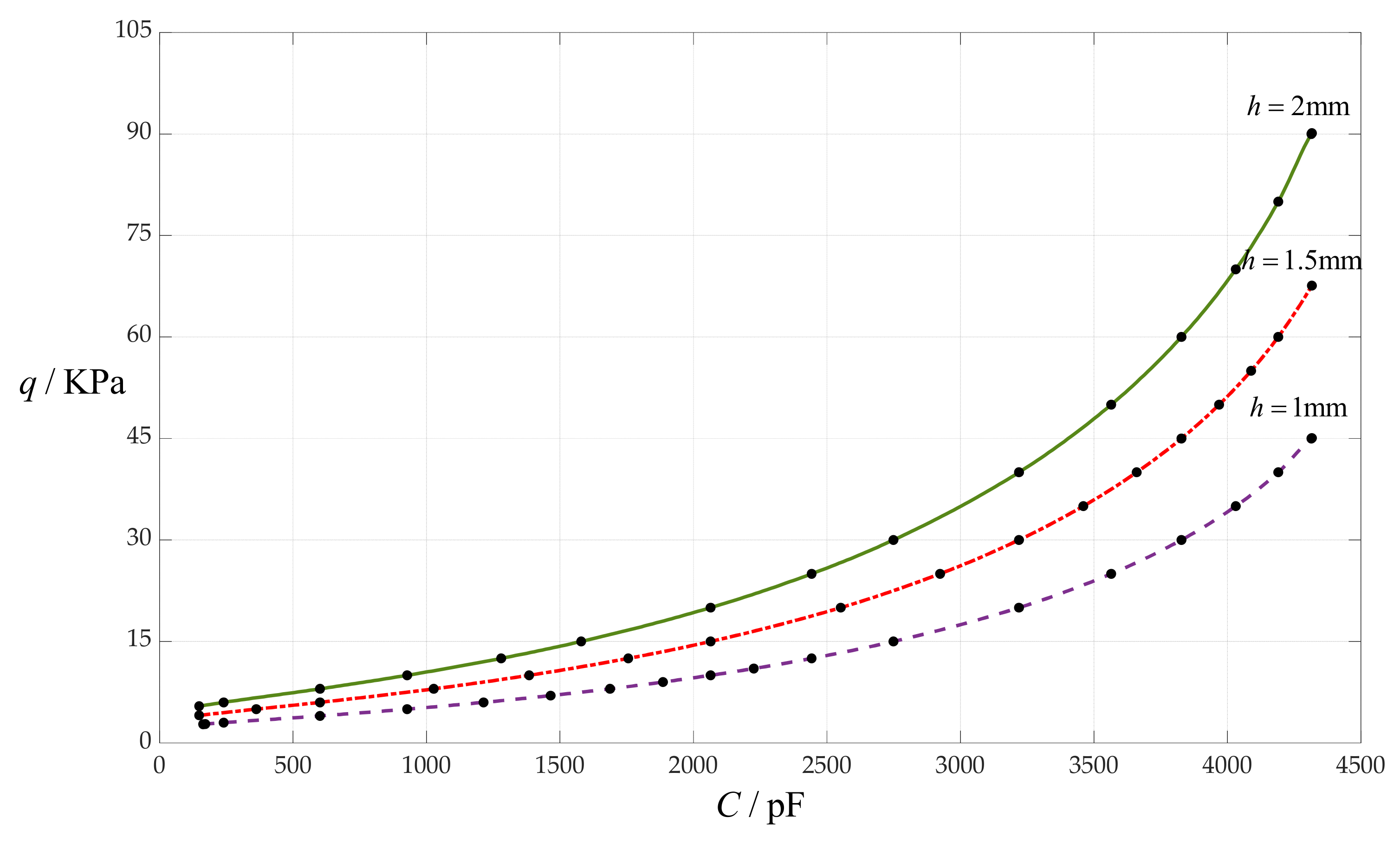
4.3. The Effect of Changing Circular Membrane Thickness h on C–q Relationships

In this section, the circular membrane thickness h takes 1 mm, 1.5 mm and 2 mm, respectively, while the other design parameters remain unchanged, that is, the circular membrane radius a = 100 mm, the initially parallel gap g = 20 mm, insulator layer thickness t = 0.1 mm, Young’s modulus of elasticity E = 7.84 MPa and Poisson’s ratio v = 0.47. In addition, the vacuum permittivity is still ε0 = 8.854 × 10⁻³ pF/mm, the relative permittivity of the insulator layer (polystyrene) is εr1 = 2.7, and the air relative permittivity is εr2 = 1.00053. The calculation results of the total capacitances C under different pressures q are listed in Table 1 when h = 1 mm, in Table 5 when h = 1.5 mm and in Table 6 when h = 2 mm. The effect of changing the circular membrane thickness h on the Cq relationships is shown in Figure 8.
From Figure 8, it can be seen that decreasing the circular membrane thickness h can decrease the output pressure range, and does not change the input capacitance range, so it can decrease the nonlinear strength of the Cq relationships.

4.4. The Effect of Changing Young’s Modulus of Elasticity E on C–q Relationships

In this section, Young’s modulus of elasticity E takes 7.84 MPa, 5 MPa and 2.5 MPa, respectively, while the other design parameters remain unchanged, that is, the circular membrane radius a = 100 mm, the initially parallel gap g = 20 mm, circular membrane thickness h = 1 mm, insulator layer thickness t = 0.1 mm and Poisson’s ratio v = 0.47. In addition, the vacuum permittivity is still ε0 = 8.854 × 10⁻³ pF/mm, the relative permittivity of the insulator layer (polystyrene) is εr1 = 2.7, and the air relative permittivity is εr2 = 1.00053. The calculation results of the total capacitances C under different pressures q are listed in Table 1 when E = 7.84 MPa, in Table 7 when E = 5 MPa and in Table 8 when E = 2.5 MPa. The effect of changing Young’s modulus of elasticity E on the Cq relationships is shown in Figure 9.
From Figure 9, it can be seen that decreasing Young’s modulus of elasticity E can increase both the output pressure range and the input capacitance range, but it can also increase the nonlinear strength of the Cq relationships.

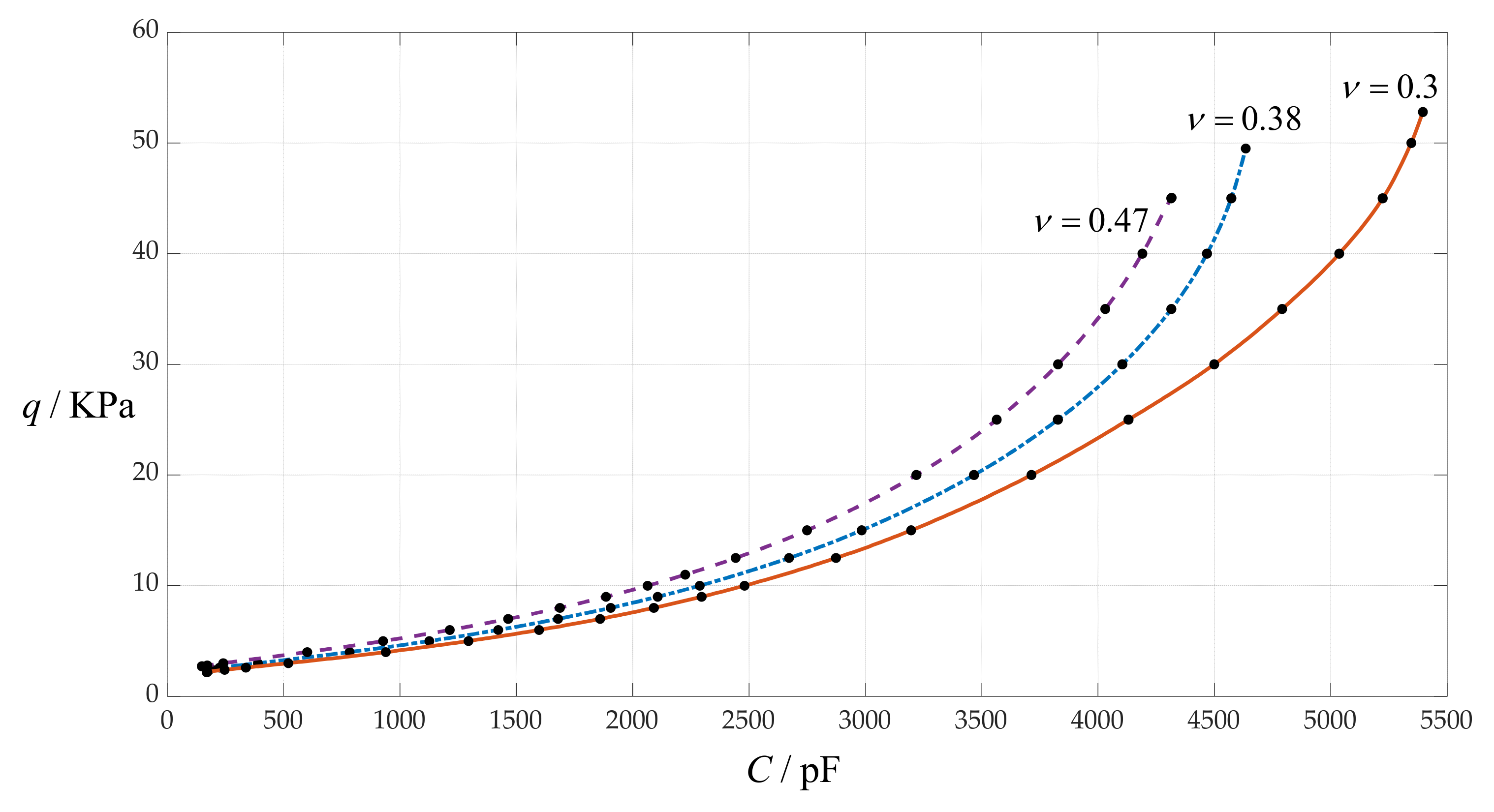
4.5. The Effect of Changing Poisson’s Ratio v on C–q Relationships

In this section, Poisson’s ratio v takes 0.47, 0.38 and 0.3, respectively, while the other design parameters remain unchanged, that is, the circular membrane radius a = 100 mm, the initially parallel gap g = 20 mm, circular membrane thickness h = 1 mm, insulator layer thickness t = 0.1 mm and Young’s modulus of elasticity E = 7.84 MPa. In addition, the vacuum permittivity is still ε0 = 8.854 × 10⁻³ pF/mm, the relative permittivity of the insulator layer (polystyrene) is εr1 = 2.7 and the air relative permittivity is εr2 = 1.00053. The calculation results of the total capacitances C under different pressures q are listed in Table 1 when v = 0.47, in Table 9 when v = 0.38 and in Table 10 when v = 0.3. The effect of changing Poisson’s ratio v on the Cq relationships is shown in Figure 10.
From Figure 10, it can be seen that decreasing Poisson’s ratio v can increase both the output pressure range and the input capacitance range, and it has little effect on the nonlinear strength of the Cq relationships.

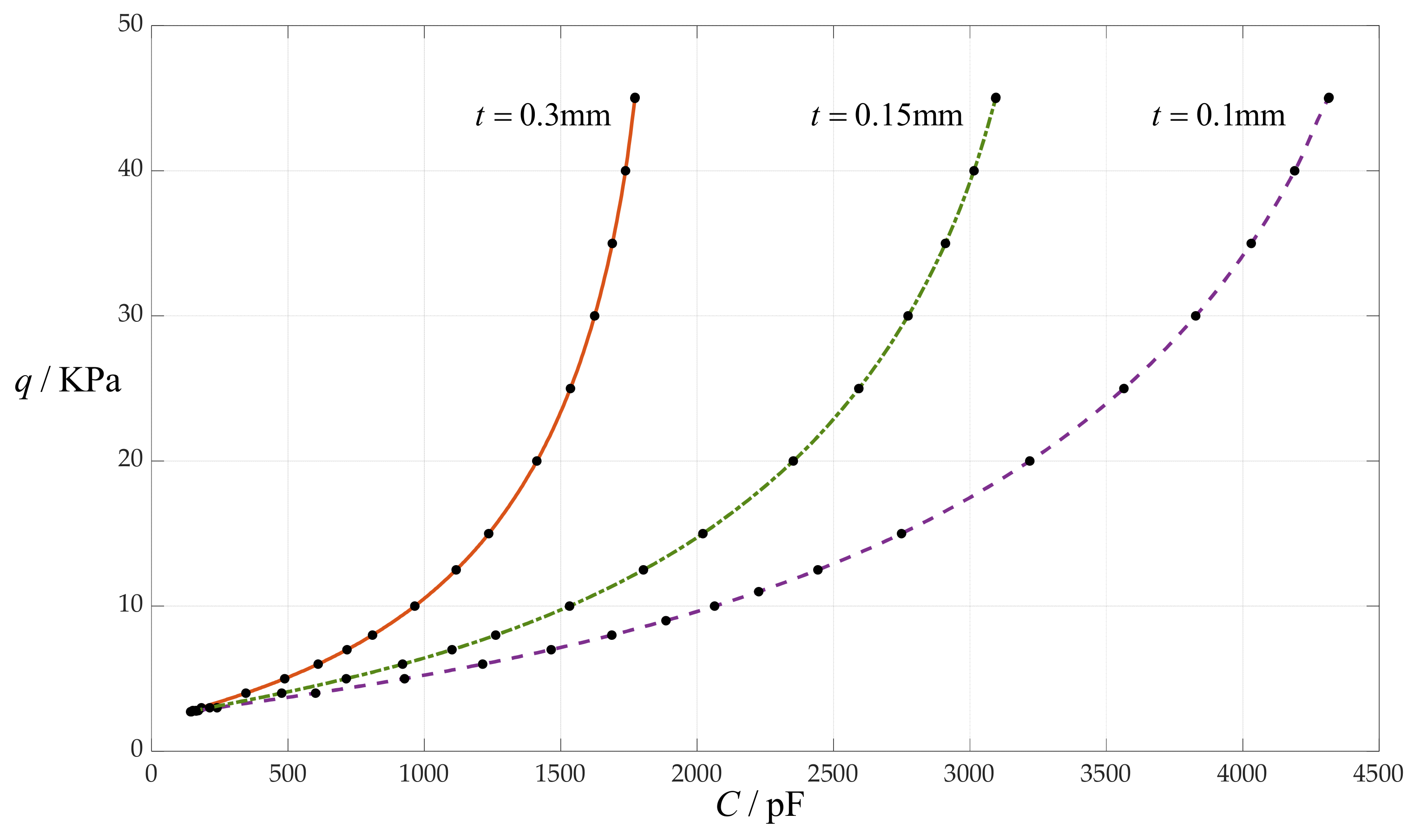
4.6. The Effect of Changing Insulator Layer Thickness t on C–q Relationships

In this section, the insulator layer thickness t takes 0.1 mm, 0.15 mm and 0.3 mm, respectively, while the other design parameters remain unchanged, that is, the circular membrane radius a = 100 mm, the initially parallel gap g = 20 mm, circular membrane thickness h = 1 mm, Young’s modulus of elasticity E = 7.84 MPa and Poisson’s ratio v = 0.47. In addition, the vacuum permittivity is still ε0 = 8.854 × 10⁻³ pF/mm, the relative permittivity of the insulator layer (polystyrene) is εr1 = 2.7 and the air relative permittivity is εr2 = 1.00053. The calculation results of the total capacitances C under different pressures q are listed in Table 1 when t = 0.1 mm, in Table 11 when t = 0.15 mm and in Table 12 when t = 0.3 mm. The effect of changing the insulator layer thickness t on the Cq relationships is shown in Figure 11.
From Figure 11, it can be seen that decreasing the insulator layer thickness t can increase the input capacitance range and does not change the output pressure range, so it can decrease the nonlinear strength of the Cq relationships.

4.7. The Effect of Changing Circular Membrane Radius a on C–q Relationships

In this section, the circular membrane radius a takes 100 mm, 90 mm and 80 mm, respectively, while the other design parameters remain unchanged, that is, the initially parallel gap g = 20 mm, circular membrane thickness h = 1 mm, insulator layer thickness t = 0.1 mm, Young’s modulus of elasticity E = 7.84 MPa and Poisson’s ratio v = 0.47. In addition, the vacuum permittivity is still ε0 = 8.854 × 10⁻³ pF/mm, the relative permittivity of the insulator layer (polystyrene) is εr1 = 2.7 and the air relative permittivity is εr2 = 1.00053. The calculation results of the total capacitances C under different pressures q are listed in Table 1 when a = 100 mm, in Table 13 when a = 90 mm and in Table 14 when a = 80 mm. The effect of changing the circular membrane radius a on the Cq relationships is shown in Figure 12.
From Figure 12, it can be seen that increasing the circular membrane radius a can increase the input capacitance range but can increase the output pressure range only a little bit, so it can decrease the nonlinear strength of the Cq relationships.

4.8. The Effect of Changing Number of Parallel Capacitors n on C–q Relationships

The parallel use of many small sensors is a relatively common technical scheme, so here we consider the case of 10, 20 and 30 small capacitors in parallel, where each small capacitor is composed of a circular membrane with radius a = 10 mm and thickness h = 0.1 mm, and the initially parallel gap g = 2 mm. The other design parameters remain unchanged, that is, the insulator layer thickness is still t = 0.1 mm, Young’s modulus of elasticity is E = 7.84 MPa, Poisson’s ratio is v = 0.47, the vacuum permittivity is ε0 = 8.854 × 10⁻³ pF/mm, the relative permittivity of the insulator layer (polystyrene) is εr1 = 2.7 and the air relative permittivity is εr2 = 1.00053. The calculation results of the total capacitances C under different pressures q are listed in Table 15. The effect of changing the number of parallel capacitors n on the Cq relationships is shown in Figure 13.
From Figure 13, it can be seen that increasing the number of parallel capacitors n can increase the input capacitance range and does not change the output pressure range, so it can decrease the nonlinear strength of the Cq relationships.

5. Concluding Remarks

In this paper, the plate/membrane axisymmetric contact problem in circular touch mode capacitive pressure sensors is reformulated using a more accurate in-plane equilibrium equation, and a new and more accurate analytical solution is presented. On this basis, the design and numerical calibration theory for circular touch mode capacitive pressure sensors has been greatly improved and perfected. Specifically, the difference between the pressure–capacitance analytical relationships calculated by the new and previous analytical solutions increases gradually with the increase in the applied pressure, showing that in comparison with the previous analytical solution, the new analytical solution is indeed significantly improved, making the design and numerical calibration theory more accurate. In addition, for the first time, this paper illustrates in detail how to use analytical solutions and analytical relationships to design and numerically calibrate a circular touch mode capacitive pressure sensor with a specified pressure detecting range. The effect of changing design parameters on capacitance–pressure analytical relationships is also comprehensively investigated for the first time, which makes clear the direction of changing design parameters to meet the required or desired range of pressure or capacitance. The changing direction of design parameters can be summarized as follows.
The decrease in the initially parallel gap g or Young’s modulus of elasticity E can increase both the output pressure range and the input capacitance range, but it can also increases the nonlinear strength of the Cq relationships.
The decrease in Poisson’s ratio v can increase both the output pressure range and the input capacitance range, and it has little effect on the nonlinear strength of the Cq relationships.
The decrease in the insulator layer thickness t or the increase in the number of parallel capacitors n can increase the input capacitance range, and does not change the output pressure range, so it can decrease the nonlinear strength of the Cq relationships.
The decrease in the circular membrane thickness h can decrease the output pressure range and does not change the input capacitance range, so it can decrease the nonlinear strength of the Cq relationships.
The increase in the circular membrane radius a can increase the input capacitance range but can only increase the output pressure range a little bit, so it can decrease the nonlinear strength of the Cq relationships.
This study makes a very positive contribution to both membrane mechanics and its technical applications: a new and more accurate analytical solution of the plate/membrane contact problem is presented for the first time, and on this basis, the design and numerical calibration theory for circular touch mode capacitive pressure sensors has been greatly improved and perfected. The work presented here can provide a better support for the design and numerical calibration of circular touch mode capacitive pressure sensors.

Author Contributions

Conceptualization, X.-T.H. and J.-Y.S.; methodology, X.-T.H., X.W., F.-Y.L. and J.-Y.S.; validation, X.-T.H. and J.-Y.S.; writing—original draft preparation, X.W. and F.-Y.L.; writing—review and editing, X.-T.H. and J.-Y.S.; visualization, X.W. and F.-Y.L.; funding acquisition, J.-Y.S. All authors have read and agreed to the published version of the manuscript.

Funding

This research was funded by the National Natural Science Foundation of China (Grant No. 11772072).

Institutional Review Board Statement

Not applicable.

Informed Consent Statement

Not applicable.

Data Availability Statement

The original contributions presented in the study are included in the article, further inquiries can be directed to the corresponding author/s.

Conflicts of Interest

The authors declare no conflict of interest.

Appendix A

b 1 = 1 β Q 2 η 2 d 1 2 8 β 2 b 0 2 d 1 2 + Q 2 η 2 4 β 2 b 0 2 ( 4 β 2 b 0 2 c 0 d 1 4 Q 2 η 2 c 0 d 1 4 + 2 Q 2 β 2 η b 0 d 1 2 + Q 2 η 2 b 0 d 1 2 2 Q 2 η 2 c 0 d 1 2 8 β 2 b 0 3 d 1 2 + 8 β 2 b 0 2 c 0 d 1 2 + 2 Q 2 β 2 η b 0 + Q 2 η 2 b 0 Q 2 η 2 c 0 4 β 2 b 0 3 + 4 β 2 b 0 2 c 0 )
b 2 = 1 2 β Q 2 η 2 d 1 2 8 β 2 b 0 2 d 1 + Q 2 η 2 4 β 2 b 0 2 ( 8 Q 2 η 2 c 0 d 1 3 d 2 Q 2 η 2 c 1 d 1 4 + 32 β 2 b 0 2 c 0 d 1 3 d 2 + 4 β 2 b 0 2 c 1 d 1 4 + 4 Q 2 β 3 b 0 d 1 2 + 16 Q 2 β 2 η b 0 d 1 d 2 + 2 Q 2 β η 2 b 1 d 1 d 2 40 β 3 b 0 2 b 1 d 1 d 2 4 β 3 b 0 b 1 2 d 1 2 + 2 Q 2 β η b 0 d 1 2 + 2 Q 2 η 2 b 0 d 1 d 2 + 2 Q 2 η 2 b 1 d 1 2 8 Q 2 η 2 c 0 d 1 d 2 2 Q 2 η 2 c 1 d 1 2 40 β 2 b 0 3 d 1 d 2 24 β 2 b 0 2 b 1 d 1 2 + 32 β 2 b 0 2 c 0 d 1 d 2 + 8 β 2 b 0 2 c 1 d 1 2 + 4 Q 2 β 3 b 0 4 β b 0 3 d 1 2 + 2 Q 2 β η b 0 + 2 Q 2 η 2 b 1 Q 2 η 2 c 1 8 β 2 b 0 2 b 1 + 4 β 2 b 0 2 c 1 )
b 3 = 1 3 β Q 2 η 2 d 1 2 8 β 2 b 0 2 d 1 2 + Q 2 η 2 4 β 2 b 0 2 ( 12 Q 2 η 2 c 0 d 1 3 d 3 24 Q 2 η 2 c 0 d 1 2 d 2 2 8 Q 2 η 2 c 1 d 1 3 d 2 Q 2 η 2 c 2 d 1 4 + 48 β 2 b 0 2 c 0 d 1 3 d 3 + 96 β 2 b 0 2 c 0 d 1 2 d 2 2 + 32 β 2 b 0 2 c 1 d 1 3 d 2 + 4 β 2 b 0 2 c 2 d 1 4 + 24 Q 2 β 3 b 0 d 1 d 2 + 36 Q 2 β 2 η b 0 d 1 d 3 + 24 Q 2 β 2 η b 0 d 2 2 + 6 Q 2 β η 2 b 2 d 1 d 2 72 β 3 b 0 2 b 1 d 1 d 3 48 β 3 b 0 2 b 1 d 2 2 72 β 3 b 0 2 b 2 d 1 d 2 24 β 3 b 0 b 1 2 d 1 d 2 12 β 3 b 0 b 1 b 2 d 1 2 + 6 Q 2 β 2 b 0 d 1 2 + 12 Q 2 β η b 0 d 1 d 2 + 6 Q 2 η 2 b 1 d 1 d 2 + 3 Q 2 η 2 b 2 d 1 2 12 Q 2 η 2 c 0 d 1 d 3 8 Q 2 η 2 c 0 d 2 2 8 Q 2 η 2 c 1 d 1 d 2 2 Q 2 η 2 c 2 d 1 2 72 β 2 b 0 3 d 1 d 3 48 β 2 b 0 3 d 2 2 120 β 2 b 0 2 b 1 d 1 d 2 36 β 2 b 0 2 b 2 d 1 2 + 48 β 2 b 0 2 c 0 d 1 d 3 + 32 β 2 b 0 2 c 0 d 2 2 + 32 β 2 b 0 2 c 1 d 1 d 2 + 8 β 2 b 0 2 c 2 d 1 2 12 β 2 b 0 b 1 2 d 1 2 24 β b 0 3 d 1 d 2 12 β b 0 2 b 1 d 1 2 + 6 Q 2 β 2 b 0 + 3 Q 2 η 2 b 2 Q 2 η 2 c 2 12 β 2 b 0 2 b 2 + 4 β 2 b 0 2 c 2 )
b 4 = 1 4 β Q 2 η 2 d 1 2 8 β 2 b 0 2 d 1 2 + Q 2 η 2 4 β 2 b 0 2 ( 16 Q 2 η 2 c 0 d 1 3 d 4 72 Q 2 η 2 c 0 d 1 2 d 2 d 3 32 Q 2 η 2 c 0 d 1 d 2 3 12 Q 2 η 2 c 1 d 1 3 d 3 24 Q 2 η 2 c 1 d 1 2 d 2 2 8 Q 2 η 2 c 2 d 1 3 d 2 Q 2 η 2 c 3 d 1 4 + 64 β 2 b 0 2 c 0 d 1 3 d 4 + 288 β 2 b 0 2 c 0 d 1 2 d 2 d 3 + 128 β 2 b 0 2 c 0 d 1 d 2 3 + 48 β 2 b 0 2 c 1 d 1 3 d 3 + 96 β 2 b 0 2 c 1 d 1 2 d 2 2 + 32 β 2 b 0 2 c 2 d 1 3 d 2 + 4 β 2 b 0 2 c 3 d 1 4 + 48 Q 2 β 3 b 0 d 1 d 3 + 32 Q 2 β 3 b 0 d 2 2 64 Q 2 β 2 η b 0 d 1 d 4 + 96 Q 2 β 2 η b 0 d 2 d 3 4 Q 2 β η 2 b 1 d 1 d 4 6 Q 2 β η 2 b 1 d 2 d 3 + 6 Q 2 β η 2 b 2 d 1 d 3 + 4 Q 2 β η 2 b 2 d 2 2 + 10 Q 2 β η 2 b 3 d 1 d 2 112 β 3 b 0 2 b 1 d 1 d 4 168 β 3 b 0 2 b 1 d 2 d 3 120 β 3 b 0 2 b 2 d 1 d 3 80 β 3 b 0 2 b 2 d 2 2 104 β 3 b 0 2 b 3 d 1 d 2 48 β 3 b 0 b 1 2 d 1 d 3 32 β 3 b 0 b 1 2 d 2 2 64 β 3 b 0 b 1 b 2 d 1 d 2 + 6 Q 2 η 2 b 1 d 1 d 3 16 β 3 b 0 b 1 b 3 d 1 2 8 β 3 b 0 b 2 2 d 1 2 + 32 Q 2 β 2 b 0 d 1 d 2 + 24 Q 2 β η b 0 d 1 d 3 + 16 Q 2 β η b 0 d 2 2 4 Q 2 η 2 b 0 d 1 d 4 6 Q 2 η 2 b 0 d 2 d 3 + 4 Q 2 η 2 b 1 d 2 2 + 10 Q 2 η 2 b 2 d 1 d 2 + 4 Q 2 η 2 b 3 d 1 2 16 Q 2 η 2 c 0 d 1 d 4 24 Q 2 η 2 c 0 d 2 d 3 12 Q 2 η 2 c 1 d 1 d 3 8 Q 2 η 2 c 1 d 2 2 8 Q 2 η 2 c 2 d 1 d 2 2 Q 2 η 2 c 3 112 β 2 b 0 3 d 1 d 4 168 β 2 b 0 3 d 2 d 3 216 β 2 b 0 2 b 1 d 1 d 3 144 β 2 b 0 2 b 1 d 2 2 168 β 2 b 0 2 b 2 d 1 d 2 48 β 2 b 0 2 b 3 d 1 2 + 64 β 2 b 0 2 c 0 d 1 d 4 + 96 β 2 b 0 2 c 0 d 2 d 3 + 48 β 2 b 0 2 c 1 d 1 d 3 + 32 β 2 b 0 2 c 1 d 2 2 + 32 β 2 b 0 2 c 2 d 1 d 2 + 8 β 2 b 0 2 c 3 d 1 2 64 β 2 b 0 b 1 2 d 1 d 2 32 β 2 b 0 b 1 b 2 d 1 2 + 2 Q 2 β b 0 d 1 2 48 β b 0 3 d 1 d 3 32 β b 0 3 d 2 2 64 β b 0 2 b 1 d 1 d 2 16 β b 0 2 b 2 d 1 2 8 β b 0 b 1 2 d 1 2 + 4 Q 2 η 2 b 3 Q 2 η 2 c 3 16 β 2 b 0 2 b 3 + 4 β 2 b 0 2 c 3 + 2 Q 2 β b 0 + d 1 2 )
b 5 = 1 5 β Q 2 η 2 d 1 2 8 β 2 b 0 2 d 1 2 + Q 2 η 2 4 β 2 b 0 2 ( 20 Q 2 η 2 c 0 d 1 3 d 5 96 Q 2 η 2 c 0 d 1 2 d 2 d 4 54 Q 2 η 2 c 0 d 1 2 d 3 2 144 Q 2 η 2 c 0 d 1 d 2 2 d 3 16 Q 2 η 2 c 0 d 2 4 16 Q 2 η 2 c 1 d 1 3 d 4 72 Q 2 η 2 c 1 d 1 2 d 2 d 3 32 Q 2 η 2 c 1 d 1 d 2 3 12 Q 2 η 2 c 2 d 1 3 d 3 24 Q 2 η 2 c 2 d 1 2 d 2 2 8 Q 2 η 2 c 3 d 1 3 d 2 Q 2 η 2 c 4 d 1 4 + 80 β 2 b 0 2 c 0 d 1 3 d 5 + 384 β 2 b 0 2 c 0 d 1 2 d 2 d 4 + 216 β 2 b 0 2 c 0 d 1 2 d 3 2 + 576 β 2 b 0 2 c 0 d 1 d 2 2 d 3 + 64 β 2 b 0 2 c 0 d 2 4 + 64 β 2 b 0 2 c 1 d 1 3 d 4 + 288 β 2 b 0 2 c 1 d 1 2 d 2 d 3 + 128 β 2 b 0 2 c 1 d 1 d 2 3 + 48 β 2 + 96 β 2 b 0 2 c 2 d 1 2 d 2 2 + 32 β 2 b 0 2 c 3 d 1 3 d 2 + 4 β 2 b 0 2 c 4 d 1 4 + 80 Q 2 β 3 b 0 d 1 d 4 + 120 Q 2 β 3 b 0 d 2 d 3 + 100 Q 2 β 2 η b 0 d 1 d 5 + 160 Q 2 β 2 η b 0 d 2 d 4 + 90 Q 2 β 2 η b 0 d 3 2 10 Q 2 β η 2 b 1 d 1 d 5 16 Q 2 β η 2 b 1 d 2 d 4 9 Q 2 β η 2 b 1 d 3 2 + 4 Q 2 β η 2 b 2 d 1 d 4 + 6 Q 2 β η 2 b 2 d 2 d 3 + 12 Q 2 β η 2 b 3 d 1 d 3 + 8 Q 2 β η 2 b 3 d 2 2 + 14 Q 2 β η 2 b 4 d 1 d 2 160 β 3 b 0 2 b 1 d 1 d 5 256 β 3 b 0 2 b 1 d 2 d 4 144 β 3 b 0 2 b 1 d 3 2 + b 0 2 c 2 d 1 3 d 3 176 β 3 b 0 2 b 2 d 1 d 4 264 β 3 b 0 2 b 2 d 2 d 3 168 β 3 b 0 2 b 3 d 1 d 3 112 β 3 b 0 2 b 3 d 2 2 136 β 3 b 0 2 b 4 d 1 d 2 80 β 3 b 0 b 1 2 d 1 d 4 120 β 3 b 0 b 1 2 d 2 d 3 120 β 3 b 0 b 1 b 2 d 1 d 3 80 β 3 b 0 b 1 b 2 d 2 2 80 β 3 b 0 b 1 b 3 d 1 d 2 20 β 3 b 0 b 1 b 4 d 1 2 40 β 3 b 0 b 2 2 d 1 d 2 20 β 3 b 0 b 2 b 3 d 1 2 + 60 Q 2 β 2 b 0 d 1 d 3 + 40 Q 2 β 2 b 0 d 2 2 + 40 Q 2 β η b 0 d 1 d 4 + 60 Q 2 β η b 0 d 2 d 3 10 Q 2 η 2 b 0 d 1 d 5 16 Q 2 η 2 b 0 d 2 d 4 9 Q 2 η 2 b 0 d 3 2 4 Q 2 η 2 b 1 d 1 d 4 + 6 Q 2 η 2 b 1 d 2 d 3 + 12 Q 2 η 2 b 2 d 1 d 3 + 8 Q 2 η 2 b 2 d 2 2 + 14 Q 2 η 2 b 3 d 1 d 2 + 5 Q 2 η 2 b 4 d 1 2 20 Q 2 η 2 c 0 d 1 d 5 32 Q 2 η 2 c 0 d 2 d 4 18 Q 2 η 2 c 0 d 3 2 16 Q 2 η 2 c 1 d 1 d 4 24 Q 2 η 2 c 1 d 2 d 3 12 Q 2 η 2 c 2 d 1 d 3 8 Q 2 η 2 c 2 d 2 2 8 Q 2 η 2 c 3 d 1 d 2 2 Q 2 η 2 c 4 d 1 2 160 β 2 b 0 3 d 1 d 5 256 β 2 b 0 3 d 2 d 4 144 β 2 b 0 3 d 3 2 336 β 2 b 0 2 b 1 d 1 d 4 504 β 2 b 0 2 b 1 d 2 d 3 288 β 2 b 0 2 b 2 d 1 d 3 192 β 2 b 0 2 b 2 d 2 2 216 β 2 60 β 2 b 0 2 b 4 d 1 2 + 80 β 2 b 0 2 c 0 d 1 d 5 + 128 β 2 b 0 2 c 0 d 2 d 4 + 72 β 2 b 0 2 c 0 d 3 2 + 64 β 2 b 0 2 c 1 d 1 d 4 + 96 β 2 b 0 2 c 1 d 2 d 3 + 48 β 2 b 0 2 c 2 d 1 d 3 + 32 β 2 b 0 2 c 2 d 2 2 + 32 β 2 b 0 2 c 3 d 1 d 2 + 8 β 2 b 0 2 c 4 d 1 2 120 β 2 b 0 b 1 2 d 1 d 3 80 β 2 b 0 b 1 2 d 2 2 160 β 2 b 0 b 1 b 2 d 1 d 2 40 β 2 b 0 b 1 b 3 d 1 2 20 β 2 b 0 b 2 2 d 1 2 + 10 Q 2 β b 0 d 1 d 2 80 β b 0 3 d 1 d 4 120 β b 0 3 d 2 d 3 120 β b 0 2 b 1 d 1 d 3 80 β b 0 2 b 1 d 2 2 80 β b 0 2 b 2 d 1 d 2 20 β b 0 2 b 3 d 1 2 + b 0 2 b 3 d 1 d 2 40 β b 0 b 1 2 d 1 d 2 20 β b 0 b 1 b 2 d 1 2 + 5 Q 2 η 2 b 4 Q 2 η 2 c 4 20 β 2 b 0 2 b 4 + 4 β 2 b 0 2 c 4 )
b 6 = 1 6 β Q 2 η 2 d 1 2 8 β 2 b 0 2 d 1 2 + Q 2 η 2 4 β 2 b 0 2 ( 24 Q 2 η 2 c 0 d 1 3 d 6 96 Q 2 η 2 c 0 d 2 3 d 3 20 Q 2 η 2 c 1 d 1 3 d 5 54 Q 2 η 2 c 1 d 1 2 d 3 2 32 Q 2 η 2 c 2 d 1 d 2 3 24 Q 2 η 2 c 3 d 1 2 d 2 2 8 Q 2 η 2 c 4 d 1 3 d 2 + 384 β 2 b 0 2 c 0 d 2 3 d 3 + 128 β 2 b 0 2 c 2 d 1 d 2 3 30 Q 2 η 2 b 0 d 2 d 5 36 Q 2 η 2 b 0 d 3 d 4 + 12 Q 2 η 2 b 2 d 1 d 4 + 18 Q 2 η 2 b 2 d 2 d 3 24 Q 2 η 2 c 0 d 1 d 6 32 Q 2 η 2 c 1 d 2 d 4 12 Q 2 η 2 c 3 d 1 d 3 8 Q 2 η 2 c 4 d 1 d 2 + 96 β 2 b 0 2 c 0 d 1 d 6 + 128 β 2 b 0 2 c 1 d 2 d 4 + 48 β 2 b 0 2 c 3 d 1 d 3 + 32 β 2 b 0 2 c 4 d 1 d 2 16 Q 2 η 2 c 2 d 1 3 d 4 + 12 Q 2 β η 2 b 4 d 2 2 18 Q 2 η 2 b 0 d 1 d 6 + 18 Q 2 η 2 b 3 d 1 d 3 + 18 Q 2 η 2 b 4 d 1 d 2 40 Q 2 η 2 c 0 d 2 d 5 48 Q 2 η 2 c 0 d 3 d 4 20 Q 2 η 2 c 1 d 1 d 5 16 Q 2 η 2 c 2 d 1 d 4 24 Q 2 η 2 c 2 d 2 d 3 + 160 β 2 b 0 2 c 0 d 2 d 5 + 192 β 2 b 0 2 c 0 d 3 d 4 + 80 β 2 b 0 2 c 1 d 1 d 5 + 64 β 2 b 0 2 c 2 d 1 d 4 + 96 β 2 b 0 2 c 2 d 2 d 3 + 12 β b 0 Q 2 d 2 2 108 β b 0 3 d 3 2 72 β b 0 b 1 2 d 1 d 3 48 β b 0 b 1 2 d 2 2 + 6 Q 2 η 2 b 5 Q 2 η 2 c 5 24 β 2 b 0 2 b 5 + 4 β 2 b 0 2 c 5 16 Q 2 η 2 c 1 d 2 4 Q 2 η 2 c 5 d 1 4 + 64 β 2 b 0 2 c 1 d 2 4 + 4 β 2 b 0 2 c 5 d 1 4 + 108 β 3 b 0 Q 2 d 3 2 216 β 3 b 0 2 b 2 d 3 2 144 β 3 b 0 2 b 4 d 2 2 108 β 3 b 0 b 1 2 d 3 2 48 β 3 b 0 b 2 2 d 2 2 12 β 3 b 0 b 3 2 d 1 2 + 12 Q 2 η 2 b 3 d 2 2 + 6 Q 2 η 2 b 5 d 1 2 18 Q 2 η 2 c 1 d 3 2 8 Q 2 η 2 c 3 d 2 2 2 Q 2 η 2 c 5 d 1 2 216 β 2 b 0 3 d 1 d 6 360 β 2 b 0 3 d 2 d 5 432 β 2 b 0 3 d 3 d 4 432 β 2 b 0 2 b 1 d 3 2 240 β 2 b 0 2 b 3 d 2 2 72 β 2 b 0 2 b 5 d 1 2 + 72 β 2 b 0 2 c 1 d 3 2 + 32 β 2 b 0 2 c 3 d 2 2 + 8 β 2 b 0 2 c 5 d 1 2 12 β b 0 b 2 2 d 1 2 120 Q 2 η 2 c 0 d 1 2 d 2 d 5 96 Q 2 η 2 c 1 d 1 2 d 2 d 4 144 Q 2 η 2 c 1 d 1 d 2 2 d 3 72 Q 2 η 2 c 2 d 1 2 d 2 d 3 + 576 β 2 b 0 2 c 1 d 1 d 2 2 d 3 18 Q 2 β η 2 b 1 d 1 d 6 30 Q 2 β η 2 b 1 d 2 d 5 36 Q 2 β η 2 b 1 d 3 d 4 + 12 Q 2 β η 2 b 3 d 1 d 4 + 18 Q 2 β η 2 b 3 d 2 d 3 + 18 Q 2 β η 2 b 4 d 1 d 3 + 18 Q 2 β η 2 b 5 d 1 d 2 + 60 β b 0 Q 2 η d 1 d 5 + 96 β b 0 Q 2 η d 2 d 4 120 β b 0 3 d 1 d 5 192 β b 0 3 d 2 d 4 96 β b 0 2 b 2 d 2 2 24 β b 0 2 b 4 d 1 2 96 β b 0 b 1 b 2 d 1 d 2 144 Q 2 η 2 c 0 d 1 2 d 3 d 4 192 Q 2 η 2 c 0 d 1 d 2 2 d 4 216 Q 2 η 2 c 0 d 1 d 2 d 3 2 + 480 β 2 b 0 2 c 0 d 1 2 d 2 d 5 + 576 β 2 b 0 2 c 0 d 1 2 d 3 d 4 + 768 β 2 b 0 2 c 0 d 1 d 2 2 d 4 + 864 β 2 b 0 2 c 0 d 1 d 2 d 3 2 + 384 β 2 b 0 2 c 1 d 1 2 d 2 d 4 + 288 β 2 b 0 2 c 2 d 1 2 d 2 d 3 + 144 β 2 b 0 Q 2 η d 1 d 6 + 240 β 2 b 0 Q 2 η d 2 d 5 + 288 β 2 b 0 Q 2 η d 3 d 4 192 β 3 b 0 b 1 b 2 d 1 d 4 288 β 3 b 0 b 1 b 2 d 2 d 3 144 β 3 b 0 b 1 b 3 d 1 d 3 96 β 3 b 0 b 1 b 4 d 1 d 2 96 β 3 b 0 b 2 b 3 d 1 d 2 120 β 3 b 0 Q 2 d 1 d 5 + 192 β 3 b 0 Q 2 d 2 d 4 120 β 3 b 0 b 1 2 d 1 d 5 192 β 3 b 0 b 1 2 d 2 d 4 96 β 3 b 0 b 1 b 3 d 2 2 24 β 3 b 0 b 1 b 5 d 1 2 72 β 3 b 0 b 2 2 d 1 d 3 24 β 3 b 0 b 2 b 4 d 1 2 + 96 β 2 b 0 Q 2 d 1 d 4 288 β 2 b 0 b 1 b 2 d 1 d 3 192 β 2 b 0 b 1 b 2 d 2 2 192 β 2 b 0 b 1 b 3 d 1 d 2 48 β 2 b 0 b 1 b 4 d 1 2 96 β 2 b 0 b 2 2 d 1 d 2 48 β 2 b 0 b 2 b 3 d 1 2 192 β b 0 2 b 1 d 1 d 4 288 β b 0 2 b 1 d 2 d 3 144 β b 0 2 b 2 d 1 d 3 96 β b 0 2 b 3 d 1 d 2 24 β b 0 b 1 b 3 d 1 2 216 β 3 b 0 2 b 1 d 1 d 6 360 β 3 b 0 2 b 1 d 2 d 5 432 β 3 b 0 2 b 1 d 3 d 4 240 β 3 b 0 2 b 2 d 1 d 5 384 β 3 b 0 2 b 2 d 2 d 4 240 β 3 b 0 2 b 3 d 1 d 4 360 β 3 b 0 2 b 3 d 2 d 3 216 β 3 b 0 2 b 4 d 1 d 3 168 β 3 b 0 2 b 5 d 1 d 2 + 144 β 2 b 0 Q 2 d 2 d 3 + 54 β b 0 Q 2 η d 3 2 480 β 2 b 0 2 b 1 d 1 d 5 192 β 2 b 0 b 1 2 d 1 d 4 288 β 2 b 0 b 1 2 d 2 d 3 + 18 β b 0 Q 2 d 1 d 3 768 β 2 12 Q 2 η 2 c 3 d 1 3 d 3 + 96 β 2 b 0 2 c 0 d 1 3 d 6 + 80 β 2 b 0 2 c 1 d 1 3 d 5 + 216 β 2 b 0 2 c 1 d 1 2 d 3 2 + 64 β 2 b 0 2 c 2 d 1 3 d 4 + 48 β 2 b 0 2 c 3 d 1 3 d 3 + 96 β 2 b 0 2 c 3 d 1 2 d 2 2 + 32 β 2 b 0 2 c 4 d 1 3 d 2 432 β 2 b 0 2 b 2 d 1 d 4 648 β 2 b 0 2 b 2 d 2 d 3 360 β 2 b 0 2 b 3 d 1 d 3 264 β 2 b 0 2 b 4 d 1 d 2 + b 0 2 b 1 d 2 d 4 )
b 7 = 1 7 β Q 2 η 2 d 1 2 8 β 2 b 0 2 d 1 2 + Q 2 η 2 4 β 2 b 0 2 ( 864 β 2 b 0 2 c 1 d 1 d 2 d 3 2 60 Q 2 β η 2 b 1 d 3 d 5 + 10 Q 2 β η 2 b 3 d 1 d 5 + 24 Q 2 β η 2 b 5 d 1 d 3 12 Q 2 β η 2 b 2 d 3 d 4 10 Q 2 β η 2 b 2 d 2 d 5 48 Q 2 β η 2 b 1 d 2 d 6 28 Q 2 β η 2 b 1 d 1 d 7 + 30 Q 2 β η 2 b 4 d 2 d 3 + 22 Q 2 β η 2 b 6 d 1 d 2 + 2304 β 2 b 0 2 c 0 d 1 d 2 d 3 d 4 + 128 β 2 b 0 2 c 0 d 4 2 16 Q 2 η 2 c 2 d 2 4 + 64 β 2 b 0 2 c 2 d 2 4 + 8 β 2 b 0 2 d 1 2 c 6 + 4 β 2 b 0 2 d 1 4 c 6 + 126 β 2 b 0 Q 2 d 3 2 252 β 2 b 0 b 1 2 d 3 2 112 β 2 b 0 b 2 2 d 2 2 28 β 2 b 0 b 3 2 d 1 2 384 β 2 b 0 2 d 1 2 c 2 d 2 d 4 + 288 β 2 b 0 2 d 1 2 c 3 d 2 d 3 + 196 β 2 b 0 Q 2 η d 1 d 7 + 336 β 2 b 0 Q 2 η d 2 d 6 + 420 β 2 b 0 Q 2 η d 3 d 5 280 β 3 b 0 b 1 b 2 d 1 d 5 448 β 3 b 0 b 1 b 2 d 2 d 4 224 β 3 b 0 b 1 b 3 d 1 d 4 336 β 3 b 0 b 1 b 3 d 2 d 3 168 β 3 b 0 b 1 b 4 d 1 d 3 112 β 3 b 0 b 1 b 5 d 1 d 2 168 β 3 b 0 b 2 b 3 d 1 d 3 112 β 3 b 0 b 2 b 4 d 1 d 2 168 β b 0 3 d 1 d 6 280 β b 0 3 d 2 d 5 336 β b 0 3 d 3 d 4 252 β b 0 2 b 1 d 3 2 112 β b 0 2 b 3 d 2 2 96 Q 2 η 2 c 2 d 1 2 d 2 d 4 144 Q 2 η 2 c 2 d 1 d 2 2 d 3 72 Q 2 η 2 c 3 d 1 2 d 2 d 3 + 576 β 2 b 0 2 c 2 d 1 d 2 2 d 3 6 Q 2 β η 2 b 2 d 1 d 6 + 16 Q 2 β η 2 b 3 d 2 d 4 + 20 Q 2 β η 2 b 4 d 1 d 4 + 84 β b 0 Q 2 η d 1 d 6 + 140 β b 0 Q 2 η d 2 d 5 + 168 β b 0 Q 2 η d 3 d 4 448 β 2 b 0 b 1 b 2 d 1 d 4 672 β 2 b 0 b 1 b 2 d 2 d 3 336 β 2 b 0 b 1 b 3 d 1 d 3 224 β 2 b 0 b 1 b 4 d 1 d 2 224 β 2 b 0 b 2 b 3 d 1 d 2 168 β b 0 b 1 b 2 d 1 d 3 112 β b 0 b 1 b 3 d 1 d 2 144 Q 2 η 2 c 0 d 1 2 d 2 d 6 180 Q 2 η 2 c 0 d 1 2 d 3 d 5 240 Q 2 η 2 c 0 d 1 d 2 2 d 5 576 Q 2 η 2 c 0 d 1 d 2 d 3 d 4 120 Q 2 η 2 c 1 d 1 2 d 2 d 5 144 Q 2 η 2 c 1 d 1 2 d 3 d 4 192 Q 2 η 2 c 1 d 1 d 2 2 d 4 216 Q 2 η 2 c 1 d 1 d 2 d 3 2 + 576 β 2 b 0 2 d 1 2 c 0 d 2 d 6 + 720 β 2 b 0 2 d 1 2 c 0 d 3 d 5 + 960 β 2 b 0 2 c 0 d 1 d 2 2 d 5 + 480 β 2 b 0 2 d 1 2 c 1 d 2 d 5 + 576 β 2 b 0 2 d 1 2 c 1 d 3 d 4 + 768 β 2 b 0 2 c 1 d 1 d 2 2 d 4 304 β 3 b 0 2 b 4 d 1 d 4 320 β 2 b 0 3 d 4 2 + 7 Q 2 η 2 b 6 Q 2 η 2 c 6 28 β 2 b 0 2 b 6 + 4 β 2 b 0 2 c 6 456 β 3 b 0 2 b 4 d 2 d 3 264 β 3 b 0 2 b 5 d 1 d 3 200 β 3 b 0 2 b 6 d 1 d 2 648 β 2 b 0 2 b 1 d 1 d 6 1080 β 2 b 0 2 b 1 d 2 d 5 1296 β 2 b 0 2 b 1 d 3 d 4 600 β 2 b 0 2 b 2 d 1 d 5 960 β 2 b 0 2 b 2 d 2 d 4 528 β 2 b 0 2 b 3 d 1 d 4 792 β 2 b 0 2 b 3 d 2 d 3 432 β 2 b 0 2 b 4 d 1 d 3 312 β 2 b 0 2 b 5 d 1 d 2 + 28 β b 0 Q 2 d 1 d 4 + 42 β b 0 Q 2 d 2 d 3 112 β b 0 b 1 2 d 1 d 4 168 β b 0 b 1 2 d 2 d 3 112 β b 0 b 1 b 2 d 2 2 28 β b 0 b 1 b 4 d 1 2 56 β b 0 b 2 2 d 1 d 2 28 β b 0 b 2 b 3 d 1 2 28 β b 0 2 b 5 d 1 2 320 β 3 b 0 2 b 1 d 4 2 288 β 3 b 0 2 b 3 d 3 2 176 β 3 b 0 2 b 5 d 2 2 280 β 2 b 0 3 d 1 d 7 480 β 2 b 0 3 d 2 d 6 600 β 2 b 0 3 d 3 d 5 540 β 2 b 0 2 b 2 d 3 2 288 β 2 b 0 2 b 4 d 2 2 84 β 2 b 0 2 b 6 d 1 2 + 7 Q 2 η 2 b 6 d 1 2 + 16 Q 2 η 2 b 4 d 2 2 + 9 Q 2 η 2 b 2 d 3 2 32 Q 2 η 2 b 0 d 4 2 Q 2 η 2 c 6 d 1 4 2 Q 2 η 2 c 6 d 1 2 8 Q 2 η 2 c 4 d 2 2 + 32 β 2 b 0 2 c 4 d 2 2 18 Q 2 η 2 c 2 d 3 2 + 72 β 2 b 0 2 c 2 d 3 2 32 Q 2 η 2 c 0 d 4 2 20 Q 2 η 2 c 2 d 1 3 d 5 20 Q 2 η 2 c 2 d 1 d 5 + 80 β 2 b 0 2 c 2 d 1 d 5 96 Q 2 η 2 c 1 d 2 3 d 3 32 Q 2 η 2 c 3 d 1 d 2 3 12 Q 2 η 2 c 4 d 1 3 d 3 8 Q 2 η 2 c 5 d 1 3 d 2 + 384 β 2 b 0 2 c 1 d 2 3 d 3 + 128 β 2 b 0 2 c 3 d 1 d 2 3 28 Q 2 η 2 b 0 d 1 d 7 48 Q 2 η 2 b 0 d 2 d 6 6 Q 2 η 2 b 1 d 1 d 6 10 Q 2 η 2 b 1 d 2 d 5 12 Q 2 η 2 b 1 d 3 d 4 + 10 Q 2 η 2 b 2 d 1 d 5 + 16 Q 2 η 2 b 2 d 2 d 4 + 20 Q 2 η 2 b 3 d 1 d 4 12 Q 2 η 2 c 4 d 1 d 3 8 Q 2 η 2 c 5 d 1 d 2 + 48 β 2 b 0 2 c 4 d 1 d 3 + 32 β 2 b 0 2 c 5 d 1 d 2 280 β b 0 2 b 1 d 1 d 5 448 β b 0 2 b 1 d 2 d 4 224 β b 0 2 b 2 d 1 d 4 + 168 β 3 b 0 Q 2 d 1 d 6 + 280 β 3 b 0 Q 2 d 2 d 5 + 336 β 3 b 0 Q 2 d 3 d 4 + 224 β 2 b 0 Q 2 η d 4 2 168 β 3 b 0 b 1 2 d 1 d 6 280 β 3 b 0 b 1 2 d 2 d 5 336 β 3 b 0 b 1 2 d 3 d 4 252 β 3 b 0 b 1 b 2 d 3 2 112 β 3 b 0 b 1 b 4 d 2 2 28 β 3 b 0 b 1 b 6 d 1 2 112 β 3 b 0 b 2 2 d 1 d 4 168 β 3 b 0 b 2 2 d 2 d 3 112 β 3 b 0 b 2 b 3 d 2 2 28 β 3 b 0 b 2 b 5 d 1 2 56 β 3 b 0 b 3 2 d 1 d 2 28 β 3 b 0 b 3 b 4 d 1 2 + 140 β 2 b 0 Q 2 d 1 d 5 336 β b 0 2 b 2 d 2 d 3 168 β b 0 2 b 3 d 1 d 3 112 β b 0 2 b 4 d 1 d 2 96 Q 2 η 2 c 0 d 1 2 d 4 2 24 Q 2 η 2 c 1 d 1 3 d 6 54 Q 2 η 2 c 2 d 1 2 d 3 2 24 Q 2 η 2 c 4 d 1 2 d 2 2 + 224 β 2 b 0 Q 2 d 2 d 4 60 Q 2 η 2 b 0 d 3 d 5 60 Q 2 η 2 c 0 d 3 d 5 24 Q 2 η 2 c 1 d 1 d 6 40 Q 2 η 2 c 1 d 2 d 5 48 Q 2 η 2 c 1 d 3 d 4 + 240 β 2 b 0 2 c 0 d 3 d 5 + 96 β 2 b 0 2 c 1 d 1 d 6 + 160 β 2 b 0 2 c 1 d 2 d 5 + 192 β 2 b 0 2 c 1 d 3 d 4 280 β 2 b 0 b 1 2 d 1 d 5 448 β 2 b 0 b 1 2 d 2 d 4 224 β 2 b 0 b 1 b 3 d 2 2 56 β 2 b 0 b 1 b 5 d 1 2 168 β 2 b 0 b 2 2 d 1 d 3 56 β 2 b 0 b 2 b 4 d 1 2 28 Q 2 η 2 c 0 d 1 3 d 7 108 Q 2 η 2 c 0 d 1 d 3 3 16 Q 2 η 2 c 3 d 1 3 d 4 + 432 β 2 b 0 2 c 0 d 1 d 3 3 32 Q 2 β η 2 b 1 d 4 2 + 9 Q 2 β η 2 b 3 d 3 2 + 16 Q 2 β η 2 b 5 d 2 2 + 30 Q 2 η 2 b 3 d 2 d 3 + 24 Q 2 η 2 b 4 d 1 d 3 + 22 Q 2 η 2 b 5 d 1 d 2 28 Q 2 η 2 c 0 d 1 d 7 48 Q 2 η 2 c 0 d 2 d 6 32 Q 2 η 2 c 2 d 2 d 4 16 Q 2 η 2 c 3 d 1 d 4 24 Q 2 η 2 c 3 d 2 d 3 + 112 β 2 b 0 2 c 0 d 1 d 7 + 192 β 2 b 0 2 c 0 d 2 d 6 + 128 β 2 b 0 2 c 2 d 2 d 4 + 64 β 2 b 0 2 c 3 d 1 d 4 + 96 β 2 b 0 2 c 3 d 2 d 3 128 Q 2 η 2 c 0 d 2 3 d 4 216 Q 2 η 2 c 0 d 2 2 d 3 2 + 112 β 2 b 0 2 d 1 3 c 0 d 7 + 384 β 2 b 0 2 d 1 2 c 0 d 4 2 + 512 β 2 b 0 2 c 0 d 2 3 d 4 + 864 β 2 b 0 2 c 0 d 2 2 d 3 2 + 96 β 2 b 0 2 d 1 3 c 1 d 6 + 80 β 2 b 0 2 d 1 3 c 2 d 5 + 216 β 2 b 0 2 d 1 2 c 2 d 3 2 + 64 β 2 b 0 2 d 1 3 c 3 d 4 + 48 β 2 b 0 2 d 1 3 c 4 d 3 + 96 β 2 b 0 2 d 1 2 c 4 d 2 2 + 32 β 2 b 0 2 d 1 3 c 312 β 3 b 0 2 b 2 d 1 d 6 520 β 3 b 0 2 b 2 d 2 d 5 624 β 3 b 0 2 b 2 d 3 d 4 320 β 3 b 0 2 b 3 d 1 d 5 512 β 3 b 0 2 b 3 d 2 d 4 5 d 2 280 β 3 b 0 2 b 1 d 1 d 7 480 β 3 b 0 2 b 1 d 2 d 6 600 β 3 d 3 3 b 0 2 b 1 d 3 d 5 )
b 8 = 1 8 β Q 2 η 2 d 1 2 8 β 2 b 0 2 d 1 2 + Q 2 η 2 4 β 2 b 0 2 ( 432 Q 2 η 2 c 0 d 1 d 3 2 d 4 576 Q 2 η 2 c 0 d 2 2 d 3 d 4 240 Q 2 η 2 c 1 d 1 d 2 2 d 5 192 Q 2 η 2 c 2 d 1 d 2 2 d 4 + 1536 β 2 b 0 2 c 0 d 1 d 2 d 4 2 + 1728 β 2 b 0 2 c 0 d 1 d 3 2 d 4 + 2304 β 2 b 0 2 c 0 d 2 2 d 3 d 4 + 960 β 2 b 0 2 c 1 d 1 d 2 2 d 5 + 768 β 2 b 0 2 c 2 d 1 d 2 2 d 4 40 Q 2 β η 2 b 1 d 1 d 8 70 Q 2 β η 2 b 1 d 2 d 7 90 Q 2 β η 2 b 1 d 3 d 6 100 Q 2 β η 2 b 1 d 4 d 5 30 Q 2 β η 2 b 2 d 3 d 5 + 6 Q 2 β η 2 b 3 d 1 d 6 + 12 Q 2 β η 2 b 3 d 3 d 4 + 20 Q 2 β η 2 b 4 d 1 d 5 384 β 3 b 0 b 1 b 4 d 2 d 3 + 256 β 2 b 0 Q 2 η d 1 d 8 192 β 3 b 0 b 1 b 5 d 1 d 3 128 β 3 b 0 b 1 b 6 d 1 d 2 256 β 3 b 0 b 2 b 3 d 1 d 4 384 β 3 b 0 b 2 b 3 d 2 d 3 192 β 3 b 0 b 2 b 4 d 1 d 3 128 β 3 b 0 b 2 b 5 d 1 d 2 128 β 3 b 0 b 3 b 4 d 1 d 2 640 β 2 b 0 b 1 b 2 d 1 d 5 1024 β 2 b 0 b 1 b 2 d 2 d 4 512 β 2 b 0 b 1 b 3 d 1 d 4 768 β 2 b 0 b 1 b 3 d 2 d 3 384 β 2 b 0 b 1 b 4 d 1 d 3 256 β 2 b 0 b 1 b 5 d 1 d 2 384 β 2 b 0 b 2 b 3 d 1 d 3 256 β 2 b 0 b 2 b 4 d 1 d 2 216 Q 2 η 2 c 0 d 1 2 d 3 d 6 28 Q 2 η 2 c 1 d 1 3 d 7 24 Q 2 η 2 c 2 d 1 3 d 6 120 Q 2 η 2 c 2 d 1 2 d 2 d 5 54 Q 2 η 2 c 3 d 1 2 d 3 2 + 448 β 2 b 0 Q 2 η d 2 d 7 + 576 β 2 b 0 Q 2 η d 3 d 6 + 640 β 2 b 0 Q 2 η d 4 d 5 + 20 Q 2 β η 2 b 6 d 2 2 40 Q 2 η 2 b 0 d 1 d 8 70 Q 2 η 2 b 0 d 2 d 7 14 Q 2 η 2 b 1 d 1 d 7 24 Q 2 η 2 b 1 d 2 d 6 30 Q 2 η 2 b 1 d 3 d 5 + 12 Q 2 η 2 b 2 d 3 d 4 + 20 Q 2 η 2 b 3 d 1 d 5 + 32 Q 2 η 2 b 3 d 2 d 4 + 28 Q 2 η 2 b 4 d 1 d 4 72 Q 2 η 2 c 0 d 3 d 6 + 288 β 2 b 0 2 c 0 d 3 d 6 160 Q 2 η 2 c 0 d 2 3 d 5 + 640 β 2 b 0 2 c 0 d 2 3 d 5 + 224 β 3 b 0 Q 2 d 1 d 7 + 384 β 3 b 0 Q 2 d 2 d 6 + 480 β 3 b 0 Q 2 d 3 d 5 224 β 3 b 0 b 1 2 d 1 d 7 384 β 3 b 0 b 1 2 d 2 d 6 480 β 3 b 0 b 1 2 d 3 d 5 288 β 3 b 0 b 1 b 3 d 3 2 128 β 3 b 0 b 1 b 5 d 2 2 32 β 3 b 0 b 1 b 7 d 1 2 160 β 3 b 0 b 2 2 d 1 d 5 384 β b 0 2 b 1 d 1 d 6 640 β b 0 2 b 1 d 2 d 5 768 β b 0 2 b 1 d 3 d 4 320 β b 0 2 b 2 d 1 d 5 512 β b 0 2 b 2 d 2 d 4 256 β b 0 2 b 3 d 1 d 4 384 β b 0 2 b 3 d 2 d 3 192 β b 0 2 b 4 d 1 d 3 128 β b 0 2 b 5 d 1 d 2 + 112 β 2 b 0 2 d 1 3 c 1 d 7 + 96 β 2 b 0 2 d 1 3 c 2 d 6 + 80 β 2 b 0 2 d 1 3 c 3 d 5 + 64 β 2 b 0 2 d 1 3 c 4 d 4 368 β 3 b 0 2 b 5 d 1 d 4 552 β 3 b 0 2 b 5 d 2 d 3 312 β 3 b 0 2 b 6 d 1 d 3 232 β 3 b 0 2 b 7 d 1 d 2 256 β 3 b 0 b 2 2 d 2 d 4 128 β 3 b 0 b 2 b 4 d 2 2 32 β 3 b 0 b 2 b 6 d 1 2 96 β 3 b 0 b 3 2 d 1 d 3 32 β 3 b 0 b 3 b 5 d 1 2 840 β 2 b 0 2 b 1 d 1 d 7 1440 β 2 b 0 2 b 1 d 2 d 6 160 β b 0 b 1 2 d 1 d 5 256 β b 0 b 1 2 d 2 d 4 128 β b 0 b 1 b 3 d 2 2 32 β b 0 b 1 b 5 d 1 2 96 β b 0 b 2 2 d 1 d 3 32 β b 0 b 2 b 4 d 1 2 + 384 β 2 b 0 2 d 1 2 c 1 d 4 2 + 216 β 2 b 0 2 d 1 2 c 3 d 3 2 + 96 β 2 b 0 2 d 1 2 c 5 d 2 2 + 192 β 2 b 0 Q 2 d 1 d 6 + 320 β 2 b 0 Q 2 d 2 d 5 + 384 β 2 b 0 Q 2 d 3 d 4 + 128 β b 0 Q 2 η d 4 2 384 β 2 b 0 b 1 2 d 1 d 6 640 β 2 b 0 b 1 2 d 2 d 5 768 β 2 b 0 b 1 2 d 3 d 4 576 β 2 b 0 b 1 b 2 d 3 2 256 β 2 b 0 b 1 b 4 d 2 2 64 β 2 b 0 b 1 b 6 d 1 2 256 β 2 b 0 b 2 2 d 1 d 4 384 β 2 b 0 b 2 2 d 2 d 3 256 β 2 b 0 b 2 b 3 d 2 2 64 β 2 b 0 b 2 b 5 d 1 2 128 β 2 b 0 b 3 2 d 1 d 2 64 β 2 b 0 b 3 b 4 d 1 2 + 40 β b 0 Q 2 d 1 d 5 + 64 β b 0 Q 2 d 2 d 4 96 Q 2 η 2 c 2 d 2 3 d 3 8 Q 2 η 2 c 6 d 1 3 d 2 + 864 β 2 b 0 2 d 1 2 c 0 d 3 d 6 + 960 β 2 b 0 2 d 1 2 c 0 d 4 d 5 + 576 β 2 b 0 2 d 1 2 c 1 d 2 d 6 + 720 β 2 b 0 2 d 1 2 c 1 d 3 d 5 + 480 β 2 b 0 2 d 1 2 c 2 d 2 d 5 + 576 β 2 b 0 2 d 1 2 c 2 d 3 d 4 + 384 β 2 b 0 2 c 2 d 2 3 d 3 + 288 β 2 b 0 2 d 1 2 c 4 d 2 d 3 + 30 Q 2 η 2 b 5 d 1 d 3 56 Q 2 η 2 c 0 d 2 d 7 80 Q 2 η 2 c 0 d 4 d 5 20 Q 2 η 2 c 3 d 1 d 5 32 Q 2 η 2 c 3 d 2 d 4 16 Q 2 η 2 c 4 d 1 d 4 + 320 β 2 b 0 2 c 0 d 4 d 5 + 80 β 2 b 0 2 c 3 d 1 d 5 + 128 β 2 b 0 2 c 3 d 2 d 4 + 64 β 2 b 0 2 c 4 d 1 d 4 672 β 2 b 0 2 d 1 2 c 0 d 2 d 7 + 384 β 2 b 0 2 d 1 2 c 3 d 2 d 4 384 β 3 b 0 b 1 b 2 d 1 d 6 640 β 3 b 0 b 1 b 2 d 2 d 5 768 β 3 b 0 b 1 b 2 d 3 d 4 320 β 3 b 0 b 1 b 3 d 1 d 5 512 β 3 b 0 b 1 b 3 d 2 d 4 256 β 3 b 0 b 1 b 4 d 1 d 4 + 112 β b 0 Q 2 η d 1 d 7 + 192 β b 0 Q 2 η d 2 d 6 + 240 β b 0 Q 2 η d 3 d 5 256 β b 0 b 1 b 2 d 1 d 4 384 β b 0 b 1 b 2 d 2 d 3 192 β b 0 b 1 b 3 d 1 d 3 128 β b 0 b 1 b 4 d 1 d 2 128 β b 0 b 2 b 3 d 1 d 2 168 Q 2 η 2 c 0 d 1 2 d 2 d 7 240 Q 2 η 2 c 0 d 1 2 d 4 d 5 384 Q 2 η 2 c 0 d 1 d 2 d 4 2 144 Q 2 η 2 c 1 d 1 2 d 2 d 6 180 Q 2 η 2 c 1 d 1 2 d 3 d 5 144 Q 2 η 2 c 2 d 1 2 d 3 d 4 216 Q 2 η 2 c 2 d 1 d 2 d 3 2 96 Q 2 η 2 c 3 d 1 2 d 2 d 4 72 Q 2 η 2 c 4 d 1 2 d 2 d 3 + 864 β 2 b 0 2 c 2 d 1 d 2 d 3 2 14 Q 2 β η 2 b 2 d 1 d 7 24 Q 2 β η 2 b 2 d 2 d 6 + 10 Q 2 β η 2 b 3 d 2 d 5 + 42 Q 2 β η 2 b 5 d 2 d 3 + 30 Q 2 β η 2 b 6 d 1 d 3 + 26 Q 2 β η 2 b 7 d 1 d 2 288 Q 2 η 2 c 0 d 1 d 2 2 d 6 144 Q 2 η 2 c 3 d 1 d 2 2 d 3 + 1152 β 2 b 0 2 c 0 d 1 d 2 2 d 6 + 576 β 2 b 0 2 c 3 d 1 d 2 2 d 3 + 32 Q 2 β η 2 b 4 d 2 d 4 + 28 Q 2 β η 2 b 5 d 1 d 4 448 β 3 b 0 2 b 2 d 4 2 360 β 3 b 0 2 b 4 d 3 2 208 β 3 b 0 2 b 6 d 2 2 880 β 2 b 0 3 d 4 d 5 960 β 2 b 0 2 b 1 d 4 2 648 β 2 b 0 2 b 3 d 3 2 336 β 2 b 0 2 b 5 d 2 2 96 β 2 b 0 2 b 7 d 1 2 + 36 β b 0 Q 2 d 3 2 480 β b 0 3 d 3 d 5 288 β b 0 2 b 2 d 3 2 128 β b 0 2 b 4 d 2 2 32 β b 0 2 b 6 d 1 2 144 β b 0 b 1 2 d 3 2 64 β b 0 b 2 2 d 2 2 16 β b 0 b 3 2 d 1 2 16 Q 2 η 2 c 3 d 2 4 Q 2 η 2 c 7 d 1 4 + 64 β 2 b 0 2 c 3 d 2 4 + 4 β 2 b 0 2 d 1 4 c 7 + 256 β 3 b 0 Q 2 d 4 2 256 β 3 b 0 b 1 2 d 4 2 144 β 3 b 0 b 2 2 d 3 2 64 β 3 b 0 b 3 2 d 2 2 16 β 3 b 0 b 4 2 d 1 2 16 Q 2 η 2 b 1 d 4 2 + 18 Q 2 η 2 b 3 d 3 2 + 20 Q 2 η 2 b 5 d 2 2 32 Q 2 η 2 c 1 d 4 2 18 Q 2 η 2 c 3 d 3 2 8 Q 2 η 2 c 5 d 2 2 352 β 2 b 0 3 d 1 d 8 616 β 2 b 0 3 d 2 d 7 792 β 2 b 0 3 d 3 d 6 + 128 β 2 b 0 2 c 1 d 4 2 + 72 β 2 b 0 2 c 3 d 3 2 + 32 β 2 b 0 2 c 5 d 2 2 + 8 β 2 b 0 2 d 1 2 c 7 224 β b 0 3 d 1 d 7 384 β b 0 3 d 2 d 6 12 Q 2 η 2 c 5 d 1 3 d 3 24 Q 2 η 2 c 5 d 1 2 d 2 2 + 48 β 2 b 0 2 d 1 3 c 5 d 3 16 Q 2 β η 2 b 2 d 4 2 352 β 3 b 0 2 b 1 d 1 d 8 616 β 3 b 0 2 b 1 d 2 d 7 792 β 3 b 0 2 b 1 d 3 d 6 880 β 3 b 0 2 b 1 d 4 d 5 392 β 3 b 0 2 b 2 d 1 d 7 + 26 Q 2 η 2 b 6 d 1 d 2 + 8 Q 2 η 2 b 7 d 1 2 32 Q 2 η 2 c 0 d 1 d 8 12 Q 2 η 2 c 5 d 1 d 3 8 Q 2 η 2 c 6 d 1 d 2 2 Q 2 η 2 c 7 d 1 2 936 β 2 b 0 2 b 4 d 2 d 3 504 β 2 b 0 2 b 5 d 1 d 3 360 β 2 b 0 2 b 6 d 1 d 2 + 128 β 2 b 0 2 c 0 d 1 d 8 + 224 β 2 b 0 2 c 0 d 2 d 7 + 48 β 2 b 0 2 c 5 d 1 d 3 + 32 β 2 b 0 2 c 6 d 1 d 2 720 Q 2 η 2 c 0 d 1 d 2 d 3 d 5 16 Q 2 η 2 c 4 d 1 3 d 4 + 128 β 2 b 0 2 d 1 3 c 0 d 8 + 32 β 2 b 0 2 d 1 3 c 6 d 2 672 β 3 b 0 2 b 2 d 2 d 6 840 β 3 b 0 2 b 2 d 3 d 5 408 β 3 b 0 2 b 3 d 1 d 6 680 β 3 b 0 2 b 3 d 2 d 5 816 β 3 b 0 2 b 3 d 3 d 4 400 β 3 b 0 2 b 4 d 1 d 5 640 β 3 b 0 2 b 4 d 2 d 4 40 Q 2 η 2 c 2 d 2 d 5 1800 β 2 b 0 2 b 1 d 3 d 5 792 β 2 b 0 2 b 2 d 1 d 6 1320 β 2 b 0 2 b 2 d 2 d 5 1584 β 2 b 0 2 b 2 d 3 d 4 720 β 2 b 0 2 b 3 d 1 d 5 1152 β 2 b 0 2 b 3 d 2 d 4 624 β 2 b 0 2 b 4 d 1 d 4 + 160 β 2 b 0 2 c 2 d 2 d 5 32 Q 2 η 2 c 0 d 1 3 d 8 216 Q 2 η 2 c 0 d 2 d 3 3 108 Q 2 η 2 c 1 d 1 d 3 3 128 Q 2 η 2 c 1 d 2 3 d 4 + 864 β 2 b 0 2 c 0 d 2 d 3 3 + 432 β 2 b 0 2 c 1 d 1 d 3 3 + 512 β 2 b 0 2 c 1 d 2 3 d 4 + 18 Q 2 β η 2 b 4 d 3 2 90 Q 2 η 2 b 0 d 3 d 6 100 Q 2 η 2 b 0 d 4 d 5 28 Q 2 η 2 c 1 d 1 d 7 48 Q 2 η 2 c 1 d 2 d 6 60 Q 2 η 2 c 1 d 3 d 5 24 Q 2 η 2 c 2 d 1 d 6 48 Q 2 η 2 c 2 d 3 d 4 + 112 β 2 b 0 2 c 1 d 1 d 7 + 192 β 2 b 0 2 c 1 d 2 d 6 + 240 β 2 b 0 2 c 1 d 3 d 5 + 96 β 2 b 0 2 c 2 d 1 d 6 + 192 β 2 b 0 2 c 2 d 3 d 4 96 Q 2 η 2 c 1 d 1 2 d 4 2 576 Q 2 η 2 c 1 d 1 d 2 d 3 d 4 216 Q 2 η 2 c 1 d 2 2 d 3 2 20 Q 2 η 2 c 3 d 1 3 d 5 32 Q 2 η 2 c 4 d 1 d 2 3 + 2880 β 2 b 0 2 c 0 d 1 d 2 d 3 d 5 + 2304 β 2 b 0 2 c 1 d 1 d 2 d 3 d 4 + 864 β 2 b 0 2 c 1 d 2 2 d 3 2 + 128 β 2 b 0 2 c 4 d 1 d 2 3 + 6 Q 2 η 2 b 2 d 1 d 6 + 10 Q 2 η 2 b 2 d 2 d 5 + 42 Q 2 η 2 b 4 d 2 d 3 24 Q 2 η 2 c 4 d 2 d 3 + 96 β 2 b 0 2 c 4 d 2 d 3 256 β b 0 3 d 4 2 + 8 Q 2 η 2 b 7 Q 2 η 2 c 7 32 β 2 b 0 2 b 7 + 4 β 2 b 0 2 c 7 )
c 1 = β ν b 1 + ν b 0 c 0 1 + ν 2 c 0 2 2 ν b 0 c 0 2 ν c 0 + b 0 2 d 1 2 + 2 b 0 + 1 β
c 2 = 1 2 β β ν b 1 β c 1 + ν b 0 c 0 1 ( 2 β 2 ν 2 b 1 b 2 2 β 2 ν b 2 c 1 + 2 β ν 2 b 0 b 2 + 2 β ν 2 b 1 2 4 β ν b 1 c 1 2 β ν b 2 c 0 + 2 ν 2 b 0 b 1 ν 2 c 0 c 1 2 β ν b 2 + 2 β c 1 2 ν b 0 c 1 ν b 1 c 0 2 ν b 1 + ν c 1 b 0 b 1 + 2 c 0 c 1 + 2 d 1 d 2 b 1 + 2 c 1 )
c 3 = 1 6 β β ν b 1 β c 1 + ν b 0 c 0 1 ( 6 β 2 ν 2 b 1 b 3 + 4 β 2 ν 2 b 2 2 8 β 2 ν b 2 c 2 6 β 2 ν b 3 c 1 + 6 β ν 2 b 0 b 3 + 14 β ν 2 b 1 b 2 + 4 β 2 c 2 2 14 β ν b 1 c 2 14 β ν b 2 c 1 6 β ν b 3 c 0 + 6 ν 2 b 0 b 2 + 4 ν 2 b 1 2 2 ν 2 c 0 c 2 ν 2 c 1 2 6 β ν b 3 + 14 β c 1 c 2 4 ν b 0 c 2 6 ν b 1 c 1 4 ν b 2 c 0 6 ν b 2 + 2 ν c 2 2 b 0 b 2 b 1 2 + 6 c 0 c 2 + 4 c 1 2 + 6 d 1 d 3 + 4 d 2 2 2 b 2 + 6 c 2 )
c 4 = 1 4 β β ν b 1 β c 1 + ν b 0 c 0 1 ( 4 β 2 ν 2 b 1 b 4 + 6 β 2 ν 2 b 2 b 3 6 β 2 ν b 2 c 3 6 β 2 ν b 3 c 2 4 β 2 ν b 4 c 1 + 4 β ν 2 b 0 b 4 + 10 β ν 2 b 1 b 3 + 6 β ν 2 b 2 2 + 6 β 2 c 2 c 3 10 β ν b 1 c 3 12 β ν b 2 c 2 10 β ν b 3 c 1 4 β ν b 4 c 0 + 4 ν 2 b 0 b 3 + 6 ν 2 b 1 b 2 ν 2 c 0 c 3 ν 2 c 1 c 2 4 β ν b 4 + 10 β c 1 c 3 + 6 β c 2 2 3 ν b 0 c 3 5 ν b 1 c 2 5 ν b 2 c 1 3 ν b 3 c 0 4 ν b 3 + ν c 3 b 0 b 3 b 1 b 2 + 4 c 0 c 3 + 6 c 1 c 2 + 4 d 1 d 4 + 6 d 2 d 3 b 3 + 4 c 3 )
c 5 = 1 10 β β ν b 1 β c 1 + ν b 0 c 0 1 ( 10 β 2 ν 2 b 1 b 5 + 16 β 2 ν 2 b 2 b 4 + 9 β 2 ν 2 b 3 2 16 β 2 ν b 2 c 4 18 β 2 ν b 3 c 3 16 β 2 ν b 4 c 2 10 β 2 ν b 5 c 1 + 10 β ν 2 b 0 b 5 + 26 β ν 2 b 1 b 4 + 34 β ν 2 b 2 b 3 + 16 β 2 c 2 c 4 + 9 β 2 c 3 2 26 β ν b 1 c 4 34 β ν b 2 c 3 34 β ν b 3 c 2 26 β ν b 4 c 1 10 β ν b 5 c 0 + 10 ν 2 b 0 b 4 + 16 ν 2 b 1 b 3 + 9 ν 2 b 2 2 2 ν 2 c 0 c 4 2 ν 2 c 1 c 3 ν 2 c 2 2 10 β ν b 5 + 26 β c 1 c 4 + 34 β c 2 c 3 8 ν b 0 c 4 14 ν b 1 c 3 16 ν b 2 c 2 14 ν b 3 c 1 8 ν b 4 c 0 10 ν b 4 + 2 ν c 4 2 b 0 b 4 2 b 1 b 3 b 2 2 + 10 c 0 c 4 + 16 c 1 c 3 + 9 c 2 2 + 10 d 1 d 5 + 16 d 2 d 4 + 9 d 3 2 2 b 4 + 10 c 4 )
c 6 = 1 6 β β ν b 1 β c 1 + ν b 0 c 0 1 ( 6 β 2 ν 2 b 1 b 6 + 10 β 2 ν 2 b 2 b 5 + 12 β 2 ν 2 b 3 b 4 10 β 2 ν b 2 c 5 12 β 2 ν b 3 c 4 12 β 2 ν b 4 c 3 10 β 2 ν b 5 c 2 6 β 2 ν b 6 c 1 + 6 β ν 2 b 0 b 6 + 16 β ν 2 b 1 b 5 + 22 β ν 2 b 2 b 4 + 12 β ν 2 b 3 2 + 10 β 2 c 2 c 5 + 12 β 2 c 3 c 4 16 β ν b 1 c 5 22 β ν b 2 c 4 24 β ν b 3 c 3 22 β ν b 4 c 2 16 β ν b 5 c 1 6 β ν b 6 c 0 + 6 ν 2 b 0 b 5 + 10 ν 2 b 1 b 4 + 12 ν 2 b 2 b 3 ν 2 c 0 c 5 ν 2 c 1 c 4 ν 2 c 2 c 3 6 β ν b 6 + 16 β c 1 c 5 + 22 β c 2 c 4 + 12 β c 3 2 5 ν b 0 c 5 9 ν b 1 c 4 11 ν b 2 c 3 11 ν b 3 c 2 9 ν b 4 c 1 5 ν b 5 c 0 6 ν b 5 + ν c 5 b 0 b 5 b 1 b 4 b 2 b 3 + 6 c 0 c 5 + 10 c 1 c 4 + 12 c 2 c 3 + 6 d 1 d 6 + 10 d 2 d 5 + 12 d 3 d 4 b 5 + 6 c 5 )
c 7 = 1 14 β β ν b 1 β c 1 + ν b 0 c 0 1 ( 14 β 2 ν 2 b 1 b 7 + 24 β 2 ν 2 b 2 b 6 + 30 β 2 ν 2 b 3 b 5 + 16 β 2 ν 2 b 4 2 24 β 2 ν b 2 c 6 30 β 2 ν b 3 c 5 32 β 2 ν b 4 c 4 30 β 2 ν b 5 c 3 24 β 2 ν b 6 c 2 14 β 2 ν b 7 c 1 + 14 β ν 2 b 0 b 7 + 38 β ν 2 b 1 b 6 + 54 β ν 2 b 2 b 5 + 62 β ν 2 b 3 b 4 + 24 β 2 c 2 c 6 + 30 β 2 c 3 c 5 + 16 β 2 c 4 2 38 β ν b 1 c 6 54 β ν b 2 c 5 62 β ν b 3 c 4 62 β ν b 4 c 3 54 β ν b 5 c 2 38 β ν b 6 c 1 14 β ν b 7 c 0 14 ν 2 b 0 b 6 + 24 ν 2 b 1 b 5 + 30 ν 2 b 2 b 4 + 16 ν 2 b 3 2 2 ν 2 c 0 c 6 2 ν 2 c 1 c 5 2 ν 2 c 2 c 4 ν 2 c 3 2 14 β ν b 7 + 38 β c 1 c 6 + 54 β c 2 c 5 + 62 β c 3 c 4 12 ν b 0 c 6 22 ν b 1 c 5 28 ν b 2 c 4 30 ν b 3 c 3 28 ν b 4 c 2 22 ν b 5 c 1 12 ν b 6 c 0 14 ν b 6 + 2 ν c 6 2 b 0 b 6 2 b 1 b 5 2 b 2 b 4 b 3 2 + 14 c 0 c 6 + 24 c 1 c 5 + 30 c 2 c 4 + 16 c 3 2 + 14 d 1 d 7 + 24 d 2 d 6 + 30 d 3 d 5 + 16 d 4 2 2 b 6 + 14 c 6 )
c 8 = 1 8 β β ν b 1 β c 1 + ν b 0 c 0 1 ( 8 β 2 ν 2 b 1 b 8 + 14 β 2 ν 2 b 2 b 7 + 18 β 2 ν 2 b 3 b 6 + 20 β 2 ν 2 b 4 b 5 14 β 2 ν b 2 c 7 18 β 2 ν b 3 c 6 20 β 2 ν b 4 c 5 20 β 2 ν b 5 c 4 18 β 2 ν b 6 c 3 14 β 2 ν b 7 c 2 8 β 2 ν b 8 c 1 + 8 β ν 2 b 0 b 8 + 22 β ν 2 b 1 b 7 + 32 β ν 2 b 2 b 6 + 38 β ν 2 b 3 b 5 + 20 β ν 2 b 4 2 + 14 β 2 c 2 c 7 + 18 β 2 c 3 c 6 + 20 β 2 c 4 c 5 22 β ν b 1 c 7 32 β ν b 2 c 6 38 β ν b 3 c 5 40 β ν b 4 c 4 38 β ν b 5 c 3 32 β ν b 6 c 2 22 β ν b 7 c 1 8 β ν b 8 c 0 + 8 ν 2 b 0 b 7 + 14 ν 2 b 1 b 6 + 18 ν 2 b 2 b 5 + 20 ν 2 b 3 b 4 ν 2 c 0 c 7 ν 2 c 1 c 6 ν 2 c 2 c 5 ν 2 c 3 c 4 8 β ν b 8 + 22 β c 1 c 7 + 32 β c 2 c 6 + 38 β c 3 c 5 + 20 β c 4 2 7 ν b 0 c 7 13 ν b 1 c 6 17 ν b 2 c 5 19 ν b 3 c 4 19 ν b 4 c 3 17 ν b 5 c 2 13 ν b 6 c 1 7 ν b 7 c 0 8 ν b 7 + ν c 7 b 0 b 7 b 1 b 6 b 2 b 5 b 3 b 4 + 8 c 0 c 7 + 14 c 1 c 6 + 18 c 2 c 5 + 20 c 3 c 4 + 8 d 1 d 8 + 14 d 2 d 7 + 18 d 3 d 6 + 20 d 4 d 5 b 7 + 8 c 7 )
d 1 = η Q Q 2 η 2 + 4 β 2 b 0 2
d 2 = β d 1 Q 2 η 2 d 1 2 8 β 2 b 0 2 d 1 2 + Q 2 η 2 4 β 2 b 0 2 ( 2 b 0 c 0 d 1 6 + Q 2 η d 1 4 2 b 0 2 d 1 4 4 b 0 c 0 d 1 4 + 2 Q 2 η d 1 2 + 2 b 0 d 1 4 2 b 0 c 0 d 1 2 + Q 2 η )
d 3 = 1 3 d 1 Q 2 η 2 d 1 2 8 β 2 b 0 2 d 1 2 + Q 2 η 2 4 β 2 b 0 2 ( 16 β b 0 c 0 d 1 5 d 2 2 β b 0 c 1 d 1 6 + 2 Q 2 β 2 d 1 4 + 8 Q 2 β η d 1 3 d 2 + 2 Q 2 η 2 d 1 2 d 2 2 16 β 2 b 0 2 d 1 2 d 2 2 12 β 2 b 0 b 1 d 1 3 d 2 2 β 2 b 1 2 d 1 4 + Q 2 η d 1 4 12 β b 0 2 d 1 3 d 2 4 β b 0 b 1 d 1 4 16 β b 0 c 0 d 1 3 d 2 4 β b 0 c 1 d 1 4 + 4 Q 2 β 2 d 1 2 + 8 Q 2 β η d 1 d 2 + 2 Q 2 η 2 d 2 2 8 β 2 b 0 2 d 2 2 16 β 2 b 0 b 1 d 1 d 2 2 β 2 b 1 2 d 1 2 2 b 0 2 d 1 4 + 2 Q 2 η d 1 2 16 β b 0 2 d 1 d 2 4 β b 0 b 1 d 1 2 2 β b 0 c 1 d 1 2 + 2 Q 2 β 2 2 b 0 2 d 1 2 + Q 2 η )
d 4 = 1 6 d 1 Q 2 η 2 d 1 2 8 β 2 b 0 2 d 1 2 + Q 2 η 2 4 β 2 b 0 2 ( 24 β b 0 c 0 d 1 5 d 3 48 β b 0 c 0 d 1 4 d 2 2 16 β b 0 c 1 d 1 5 d 2 2 β b 0 c 2 d 1 6 + 12 Q 2 β 2 d 1 3 d 2 + 18 Q 2 β η d 1 3 d 3 + 12 Q 2 β η d 1 2 d 2 2 + 9 Q 2 η 2 d 1 2 d 2 d 3 72 β 2 b 0 2 d 1 2 d 2 d 3 36 β 2 b 0 b 1 d 1 3 d 3 24 β 2 b 0 b 1 d 1 2 d 2 2 12 β 2 b 0 b 2 d 1 3 d 2 12 β 2 b 1 2 d 1 3 d 2 6 β 2 b 1 b 2 d 1 4 + 3 Q 2 β d 1 4 + 6 Q 2 η d 1 3 d 2 36 β b 0 2 d 1 3 d 3 24 β b 0 2 d 1 2 d 2 2 36 β b 0 b 1 d 1 3 d 2 6 β b 0 b 2 d 1 4 24 β b 0 c 0 d 1 3 d 3 16 β b 0 c 0 d 1 2 d 2 2 16 β b 0 c 1 d 1 3 d 2 4 β b 0 c 2 d 1 4 6 β b 1 2 d 1 4 + 12 Q 2 β 2 d 1 d 2 + 18 Q 2 β η d 1 d 3 12 Q 2 β η d 2 2 + 9 Q 2 η 2 d 2 d 3 36 β 2 b 0 2 d 2 d 3 36 β 2 b 0 b 1 d 1 d 3 24 β 2 b 0 b 1 d 2 2 24 β 2 b 0 b 2 d 1 d 2 12 β 2 b 1 2 d 1 d 2 6 β 2 b 1 b 2 d 1 2 12 b 0 2 d 1 3 d 2 6 b 0 b 1 d 1 4 + 6 Q 2 β d 1 2 + 6 Q 2 η d 1 d 2 36 β b 0 2 d 1 d 3 24 β b 0 2 d 2 2 48 β b 0 b 1 d 1 d 2 6 β b 0 b 2 d 1 2 2 β b 0 c 2 d 1 2 6 β b 1 2 d 1 2 12 b 0 2 d 1 d 2 6 b 0 b 1 d 1 2 + 3 Q 2 β )
d 5 = 1 10 d 1 Q 2 η 2 d 1 2 8 β 2 b 0 2 d 1 2 + Q 2 η 2 4 β 2 b 0 2 ( 32 β b 0 c 0 d 1 5 d 4 144 β b 0 c 0 d 1 4 d 2 d 3 64 β b 0 c 0 d 1 3 d 2 3 24 β b 0 c 1 d 1 5 d 3 48 β b 0 c 1 d 1 4 d 2 2 16 β b 0 c 2 d 1 5 d 2 2 β b 0 c 3 d 1 6 + 24 Q 2 β 2 d 1 3 d 3 + 16 Q 2 β 2 d 1 2 d 2 2 + 32 Q 2 β η d 1 3 d 4 + 48 Q 2 β η d 1 2 d 2 d 3 + 16 Q 2 η 2 d 1 2 d 2 d 4 + 9 Q 2 η 2 d 1 2 d 3 2 128 β 2 b 0 2 d 1 2 d 2 d 4 72 β 2 b 0 2 d 1 2 d 3 2 72 β 2 b 0 b 1 d 1 3 d 4 108 β 2 b 0 b 1 d 1 2 d 2 d 3 36 β 2 b 0 b 2 d 1 3 d 3 24 β 2 b 0 b 2 d 1 2 d 2 2 12 β 2 b 0 b 3 d 1 3 d 2 24 β 2 b 1 2 d 1 3 d 3 16 β 2 b 1 2 d 1 2 d 2 2 32 β 2 b 1 b 2 d 1 3 d 2 8 β 2 b 1 b 3 d 1 4 4 β 2 b 2 2 d 1 4 + 16 Q 2 β d 1 3 d 2 + 12 Q 2 η d 1 3 d 3 + 8 Q 2 η d 1 2 d 2 2 72 β b 0 2 d 1 3 d 4 108 β b 0 2 d 1 2 d 2 d 3 84 β b 0 b 1 d 1 3 d 3 56 β b 0 b 1 d 1 2 d 2 2 44 β b 0 b 2 d 1 3 d 2 8 β b 0 b 3 d 1 4 32 β b 0 c 0 d 1 3 d 4 48 β b 0 c 0 d 1 2 d 2 d 3 24 β b 0 c 1 d 1 3 d 3 16 β b 0 c 1 d 1 2 d 2 2 16 β b 0 c 2 d 1 3 d 2 4 β b 0 c 3 d 1 4 32 β b 1 2 16 β b 1 b 2 d 1 4 + 24 Q 2 β 2 d 1 d 3 + 16 Q 2 β 2 d 2 2 + 32 Q 2 β η d 1 d 4 + 48 Q 2 β η d 2 d 3 + 16 Q 2 η 2 d 2 d 4 + 9 Q 2 η 2 d 3 2 + Q 2 d 1 4 64 β 2 b 0 2 d 2 d 4 36 β 2 b 0 2 d 3 2 64 β 2 b 0 b 1 d 1 d 4 96 β 2 b 0 b 1 d 2 d 3 48 β 2 b 0 b 2 d 1 d 3 32 β 2 b 0 b 2 d 2 2 32 β 2 b 0 b 3 d 1 d 2 24 β 2 b 1 2 d 1 d 3 16 β 2 b 1 2 d 2 2 32 β 2 b 1 b 2 d 1 d 2 8 β 2 b 1 b 3 d 1 2 4 β 2 b 2 2 d 1 2 24 b 0 2 d 1 3 d 3 16 b 0 2 d 1 2 d 2 2 32 b 0 b 1 d 1 3 d 2 8 b 0 b 2 d 1 4 4 b 1 2 d 1 4 + d 2 d 1 3 16 Q 2 β d 1 d 2 + 12 Q 2 η d 1 d 3 + 8 Q 2 η d 2 2 64 β b 0 2 d 1 d 4 96 β b 0 2 d 2 d 3 96 β b 0 b 1 d 1 d 3 64 β b 0 b 1 d 2 2 64 β b 0 b 2 d 1 d 2 8 β b 0 b 3 d 1 2 2 β b 0 c 3 d 1 2 32 β b 1 2 d 1 d 2 16 β b 1 b 2 d 1 2 + 2 Q 2 d 1 2 24 b 0 2 d 1 d 3 16 b 0 2 d 2 2 32 b 0 b 1 d 1 d 2 8 b 0 b 2 d 1 2 4 b 1 2 d 1 2 + Q 2 )
d 6 = 1 15 d 1 Q 2 η 2 d 1 2 8 β 2 b 0 2 d 1 2 + Q 2 η 2 4 β 2 b 0 2 ( 40 β b 0 c 0 d 1 5 d 5 192 β b 0 c 0 d 1 4 d 2 d 4 108 β b 0 c 0 d 1 4 d 3 2 288 β b 0 c 0 d 1 3 d 2 2 d 3 32 β b 0 c 0 d 1 2 d 2 4 32 β b 0 c 1 d 1 5 d 4 144 β b 0 c 1 d 1 4 d 2 d 3 64 β b 0 c 1 d 1 3 d 2 3 24 β b 0 c 2 d 1 5 d 3 48 β b 0 c 2 d 1 4 d 2 2 16 β b 0 c 3 d 1 5 d 2 2 β b 0 c 4 d 1 6 + 40 Q 2 β 2 d 1 3 d 4 + 60 Q 2 β 2 d 1 2 d 2 d 3 + 50 Q 2 β η d 1 3 d 5 + 80 Q 2 β η d 1 2 d 2 d 4 + 45 Q 2 β η d 1 2 d 3 2 + 25 Q 2 η 2 d 1 2 d 2 d 5 + 30 Q 2 η 2 d 1 2 d 3 d 4 200 β 2 b 0 2 d 1 2 d 2 d 5 240 β 2 b 0 2 d 1 2 d 3 d 4 120 β 2 b 0 b 1 d 1 3 d 5 192 β 2 b 0 b 1 d 1 2 d 2 d 4 108 β 2 b 0 b 1 d 1 2 d 3 2 72 β 2 b 0 b 2 d 1 3 d 4 108 β 2 b 0 b 2 d 1 2 d 2 d 3 36 β 2 b 0 b 3 d 1 3 d 3 24 β 2 b 0 b 3 d 1 2 d 2 2 12 β 2 b 0 b 4 d 1 3 d 2 40 β 2 b 1 2 d 1 3 d 4 60 β 2 b 1 2 d 1 2 d 2 d 3 60 β 2 b 1 b 2 d 1 3 d 3 40 β 2 b 1 b 2 d 1 2 d 2 2 40 β 2 b 1 b 3 d 1 3 d 2 10 β 2 b 1 b 4 d 1 4 20 β 2 b 2 2 d 1 3 d 2 10 β 2 b 2 b 3 d 1 4 + 30 Q 2 β d 1 3 d 3 + 20 Q 2 β d 1 2 d 2 2 + 20 Q 2 η d 1 3 d 4 + 30 Q 2 η d 1 2 d 2 d 3 120 β b 0 2 d 1 3 d 5 192 β b 0 2 d 1 2 d 2 d 4 108 β b 0 2 d 1 2 d 3 2 152 β b 0 b 1 d 1 3 d 4 228 β b 0 b 1 d 1 2 d 2 d 3 96 β b 0 b 2 d 1 3 d 3 64 β b 0 b 2 d 1 2 d 2 2 52 β b 0 b 3 d 1 3 d 2 10 β b 0 b 4 d 1 4 40 β b 0 c 0 d 1 3 d 5 64 β b 0 c 0 d 1 2 d 2 d 4 36 β b 0 c 0 d 1 2 d 3 2 32 β b 0 c 1 d 1 3 d 4 48 β b 0 c 1 d 1 2 d 2 d 3 24 β b 0 c 2 d 1 3 d 3 16 β b 0 c 2 d 1 2 d 2 2 16 β b 0 c 3 d 1 3 d 2 4 β b 0 c 4 d 1 4 60 β b 1 2 d 1 3 d 3 40 β b 1 2 d 1 2 d 2 2 80 β b 1 b 2 d 1 3 d 2 20 β b 1 b 3 d 1 4 10 β b 2 2 d 1 4 + 40 Q 2 β 2 d 1 d 4 + 60 Q 2 β 2 d 2 d 3 + 50 Q 2 β η d 1 d 5 + 80 Q 2 β η d 2 d 4 + 45 Q 2 β η d 3 2 + 25 Q 2 η 2 d 2 d 5 + 30 Q 2 η 2 d 3 d 4 + 5 Q 2 d 1 3 d 2 100 β 2 b 0 2 d 2 d 5 120 β 2 b 0 2 d 3 d 4 100 β 2 b 0 b 1 d 1 d 5 160 β 2 b 0 b 1 d 2 d 4 90 β 2 b 0 b 1 d 3 2 80 β 2 b 0 b 2 d 1 d 4 120 β 2 b 0 b 2 d 2 d 3 60 β 2 b 0 b 3 d 1 d 3 40 β 2 b 0 b 3 d 2 2 40 β 2 b 0 b 4 d 1 d 2 40 β 2 b 1 2 d 1 d 4 60 β 2 b 1 2 d 2 d 3 60 β 2 b 1 b 2 d 1 d 3 40 β 2 b 1 b 2 d 2 2 40 β 2 b 1 b 3 d 1 d 2 10 β 2 b 1 b 4 d 1 2 20 β 2 b 2 2 d 1 d 2 10 β 2 b 2 b 3 d 1 2 40 b 0 2 d 1 3 d 4 60 b 0 2 d 1 2 d 2 d 3 60 b 0 b 1 d 1 3 d 3 40 b 0 b 1 d 1 2 d 2 2 40 b 0 b 2 d 1 3 d 2 10 b 0 b 3 d 1 4 20 b 1 2 d 1 3 d 2 10 b 1 b 2 d 1 4 + 30 Q 2 β d 1 d 3 + 20 Q 2 β d 2 2 + 20 Q 2 η d 1 d 4 + 30 Q 2 η d 2 d 3 100 β b 0 2 d 1 d 5 160 β b 0 2 d 2 d 4 90 β b 0 2 d 3 2 160 β b 0 b 1 d 1 d 4 240 β b 0 b 1 d 2 d 3 120 β b 0 b 2 d 1 d 3 80 β b 0 b 2 d 2 2 80 β b 0 b 3 d 1 d 2 10 β b 0 b 4 d 1 2 2 β b 0 c 4 d 1 2 60 β b 1 2 d 1 d 3 40 β b 1 2 d 2 2 80 β b 1 b 2 d 1 d 2 20 β b 1 b 3 d 1 2 10 β b 2 2 d 1 2 + 5 Q 2 d 1 d 2 40 b 0 2 d 1 d 4 60 b 0 2 d 2 d 3 60 b 0 b 1 d 1 d 3 40 b 0 b 1 d 2 2 40 b 0 b 2 d 1 d 2 10 b 0 b 3 d 1 2 20 b 1 2 d 1 d 2 10 b 1 b 2 d 1 2 )
d 7 = 1 21 d 1 Q 2 η 2 d 1 2 8 β 2 b 0 2 d 1 2 + Q 2 η 2 4 β 2 b 0 2 ( 48 β b 0 c 0 d 1 5 d 6 40 β b 0 c 1 d 1 5 d 5 108 β b 0 c 1 d 1 4 d 3 2 32 β b 0 c 1 d 1 2 d 2 4 96 β b 1 b 2 d 1 2 d 2 2 96 β b 1 b 3 d 1 3 d 2 + 54 Q 2 β 2 d 3 2 + 24 Q 2 η 2 d 4 2 96 β 2 b 0 2 d 4 2 54 β 2 b 1 2 d 3 2 48 β 2 b 1 b 4 d 1 d 2 12 β 2 b 1 b 5 d 1 2 36 β 2 b 2 2 d 1 d 3 24 β 2 b 2 2 d 2 2 48 β 2 b 2 b 3 d 1 d 2 12 β 2 b 2 b 4 d 1 2 144 b 0 b 1 d 1 2 d 2 d 3 + 27 Q 2 η d 3 2 192 β b 0 b 2 d 1 d 4 12 β b 0 b 5 d 1 2 96 β b 1 2 d 1 d 4 144 β b 1 b 2 d 1 d 3 + 6 Q 2 d 2 2 54 b 0 2 d 3 2 48 b 1 b 2 d 1 d 2 32 β b 0 c 2 d 1 5 d 4 64 β b 0 c 2 d 1 3 d 2 3 24 β b 0 c 3 d 1 5 d 3 48 β b 0 c 3 d 1 4 d 2 2 16 β b 0 c 4 d 1 5 d 2 + 96 Q 2 β 2 d 1 2 d 2 d 4 + 72 Q 2 β η d 1 3 d 6 + 36 Q 2 η 2 d 1 2 d 2 d 6 + 45 Q 2 η 2 d 1 2 d 3 d 5 288 β 2 b 0 2 d 1 2 d 2 d 6 360 β 2 b 0 2 d 1 2 d 3 d 5 180 β 2 b 0 b 1 d 1 3 d 6 120 β 2 b 0 b 2 d 1 3 d 5 108 β 2 b 0 b 2 d 1 2 d 3 2 48 β b 0 c 0 d 1 3 d 6 40 β b 0 c 1 d 1 3 d 5 36 β b 0 c 1 d 1 2 d 3 2 32 β b 0 c 2 d 1 3 d 4 24 β b 0 c 3 d 1 3 d 3 16 β b 0 c 3 d 1 2 d 2 2 16 β b 0 c 4 d 1 3 d 2 72 β 2 b 0 b 3 d 1 3 d 4 36 β 2 b 0 b 4 d 1 3 d 3 24 β 2 b 0 b 4 d 1 2 d 2 2 12 β 2 b 0 b 5 d 1 3 d 2 96 β 2 b 1 2 d 1 2 d 2 d 4 96 β 2 b 1 b 2 d 1 3 d 4 72 β 2 b 1 b 3 d 1 3 d 3 48 β 2 b 1 b 3 d 1 2 d 2 2 48 β 2 b 1 b 4 d 1 3 d 2 48 β 2 b 2 b 3 d 1 3 d 2 + 72 Q 2 β d 1 2 d 2 d 3 + 48 Q 2 η d 1 2 d 2 d 4 300 β b 0 2 d 1 2 d 2 d 5 360 β b 0 2 d 1 2 d 3 d 4 240 β b 0 b 1 d 1 3 d 5 216 β b 0 b 1 d 1 2 d 3 2 168 β b 0 b 2 d 1 3 d 4 108 β b 0 b 3 d 1 3 d 3 72 β b 0 b 3 d 1 2 d 2 2 60 β b 0 b 4 d 1 3 d 2 144 β b 1 2 d 1 2 d 2 d 3 60 Q 2 β 2 d 1 3 d 5 + 54 Q 2 β 2 d 1 2 d 3 2 + 24 Q 2 η 2 d 1 2 d 4 2 192 β 2 b 0 2 d 1 2 d 4 2 60 β 2 b 1 2 d 1 3 d 5 54 β 2 b 1 2 d 1 2 d 3 2 12 β 2 b 1 b 5 d 1 4 36 β 2 b 2 2 d 1 3 d 3 24 β 2 b 2 2 d 1 2 d 2 2 12 β 2 b 2 b 4 d 1 4 + 48 Q 2 β d 1 3 d 4 + 30 Q 2 η d 1 3 d 5 144 β b 1 b 2 d 1 3 d 3 + 60 Q 2 β 2 d 1 d 5 + 96 Q 2 β 2 d 2 d 4 72 β 2 b 0 b 4 d 1 d 3 96 β 2 b 1 b 2 d 1 d 4 6 β 2 b 3 2 d 1 2 + 48 Q 2 β d 1 d 4 + 72 Q 2 β d 2 d 3 + 30 Q 2 η d 1 d 5 + 48 Q 2 η d 2 d 4 216 β b 0 b 1 d 3 2 24 b 1 2 d 2 2 6 b 2 2 d 1 2 6 β 2 b 3 2 d 1 4 + 27 Q 2 η d 1 2 d 3 2 180 β b 0 2 d 1 3 d 6 12 β b 0 b 5 d 1 4 96 β b 1 2 d 1 3 d 4 24 β b 1 b 4 d 1 4 48 β b 2 2 d 1 3 d 2 24 β b 2 b 3 d 1 4 + 9 Q 2 d 1 3 d 3 + 6 Q 2 d 1 2 d 2 2 120 β 2 b 0 b 2 d 1 d 5 192 β 2 b 0 b 2 d 2 d 4 48 β 2 b 0 b 5 d 1 d 2 60 b 0 2 d 1 3 d 5 54 b 0 2 d 1 2 d 3 2 12 b 0 b 4 d 1 4 36 b 1 2 d 1 3 d 3 24 b 1 2 d 1 2 d 2 2 12 b 1 b 3 d 1 4 240 β b 0 b 1 d 1 d 5 96 β b 0 b 4 d 1 d 2 96 β b 1 b 2 d 2 2 96 β b 1 b 3 d 1 d 2 24 β b 1 b 4 d 1 2 48 β b 2 2 d 1 d 2 144 b 0 b 1 d 2 d 3 2 β b 0 c 5 d 1 6 + 120 Q 2 β η d 1 2 d 2 d 5 + 144 Q 2 β η d 1 2 d 3 d 4 300 β 2 b 0 b 1 d 1 2 d 2 d 5 4 β b 0 c 5 d 1 4 + 36 Q 2 η 2 d 2 d 6 + 45 Q 2 η 2 d 3 d 5 144 β 2 b 0 2 d 2 d 6 180 β 2 b 0 2 d 3 d 5 108 β 2 b 0 b 2 d 3 2 144 β 2 b 1 b 2 d 2 d 3 96 b 0 2 d 1 2 d 2 d 4 96 b 0 b 1 d 1 3 d 4 72 b 0 b 2 d 1 3 d 3 48 b 0 b 2 d 1 2 d 2 2 48 b 0 b 3 d 1 3 d 2 48 b 1 b 2 d 1 3 d 2 144 β b 0 2 d 1 d 6 240 β b 0 2 d 2 d 5 288 β b 0 2 d 3 d 4 144 β b 0 b 3 d 1 d 3 2 β b 0 c 5 d 1 2 72 b 0 b 2 d 1 d 3 240 β b 0 c 0 d 1 4 d 2 d 5 288 β b 0 c 0 d 1 4 d 3 d 4 384 β b 0 c 0 d 1 3 d 2 2 d 4 432 β b 0 c 0 d 1 3 d 2 d 3 2 192 β b 0 c 0 d 1 2 d 2 3 d 3 192 β b 0 c 1 d 1 4 d 2 d 4 288 β b 0 c 1 d 1 3 d 2 2 d 3 144 β b 0 c 2 d 1 4 d 2 d 3 360 β 2 b 0 b 1 d 1 2 d 3 d 4 192 β 2 b 0 b 2 d 1 2 d 2 d 4 108 β 2 b 0 b 3 d 1 2 d 2 d 3 144 β 2 b 1 b 2 d 1 2 d 2 d 3 384 β b 0 b 1 d 1 2 d 2 d 4 252 β b 0 b 2 d 1 2 d 2 d 3 80 β b 0 c 0 d 1 2 d 2 d 5 96 β b 0 c 0 d 1 2 d 3 d 4 64 β b 0 c 1 d 1 2 d 2 d 4 48 β b 0 c 2 d 1 2 d 2 d 3 72 Q 2 β η d 1 d 6 + 120 Q 2 β η d 2 d 5 + 144 Q 2 β η d 3 d 4 96 β 2 b 0 b 3 d 1 d 4 144 β 2 b 0 b 3 d 2 d 3 48 β 2 b 0 b 4 d 2 2 60 β 2 b 1 2 d 1 d 5 96 β 2 b 1 2 d 2 d 4 72 β 2 b 1 b 3 d 1 d 3 48 β 2 b 1 b 3 d 2 2 6 b 2 2 d 1 4 384 β b 0 b 1 d 2 d 4 288 β b 0 b 2 d 2 d 3 144 β b 1 2 d 2 d 3 24 β b 2 b 3 d 1 2 96 b 0 b 1 d 1 d 4 48 b 0 b 3 d 1 d 2 12 b 1 b 3 d 1 2 144 β 2 b 0 b 1 d 1 d 6 240 β 2 b 0 b 1 d 2 d 5 288 β 2 b 0 b 1 d 3 d 4 96 β b 0 b 3 d 2 2 + 9 Q 2 d 1 d 3 60 b 0 2 d 1 d 5 96 b 0 2 d 2 d 4 48 b 0 b 2 d 2 2 12 b 0 b 4 d 1 2 36 b 1 2 d 1 d 3 )
d 8 = 1 28 d 1 Q 2 η 2 d 1 2 8 β 2 b 0 2 d 1 2 + Q 2 η 2 4 β 2 b 0 2 ( 192 β b 0 d 1 2 c 1 d 2 3 d 3 192 β b 0 d 1 4 c 2 d 2 d 4 + 168 Q 2 β η d 1 2 d 2 d 6 + 210 Q 2 β η d 1 2 d 3 d 5 432 β 2 b 0 b 1 d 1 2 d 2 d 6 540 β 2 b 0 b 1 d 1 2 d 3 d 5 300 β 2 b 0 b 2 d 1 2 d 2 d 5 360 β 2 b 0 b 2 d 1 2 d 3 d 4 192 β 2 b 0 b 3 d 1 2 d 2 d 4 108 β 2 b 0 b 4 d 1 2 d 2 d 3 224 β 2 b 1 b 2 d 1 2 d 2 d 4 168 β 2 b 1 b 3 d 1 2 d 2 d 3 580 β b 0 b 1 d 1 2 d 2 d 5 696 β b 0 b 1 d 1 2 d 3 d 4 416 β b 0 b 2 d 1 2 d 2 d 4 276 β b 0 b 3 d 1 2 d 2 d 3 96 β b 0 d 1 2 c 1 d 3 d 4 336 β b 1 b 2 d 1 2 d 2 d 3 288 β b 0 d 1 4 c 0 d 2 d 6 360 β b 0 d 1 4 c 0 d 3 d 5 480 β b 0 d 1 3 c 0 d 2 2 d 5 1152 β b 0 d 1 3 c 0 d 2 d 3 d 4 240 β b 0 d 1 4 c 1 d 2 d 5 288 β b 0 d 1 4 c 1 d 3 d 4 384 β b 0 d 1 3 c 1 d 2 2 d 4 432 β b 0 d 1 3 c 1 d 2 d 3 2 288 β b 0 d 1 3 c 2 d 2 2 d 3 144 β b 0 d 1 4 c 3 d 2 d 3 120 β b 0 d 1 2 c 0 d 3 d 5 80 β b 0 d 1 2 c 1 d 2 d 5 126 β 2 b 1 b 2 d 3 2 56 β 2 b 1 b 4 d 2 2 14 β 2 b 1 b 6 d 1 2 56 β 2 b 2 2 d 1 d 4 84 β 2 b 2 2 d 2 d 3 56 β 2 b 2 b 3 d 2 2 14 β 2 b 2 b 5 d 1 2 28 β 2 b 3 2 d 1 d 2 14 β 2 b 3 b 4 d 1 2 + 70 Q 2 β d 1 d 5 + 112 Q 2 β d 2 d 4 + 42 Q 2 η d 1 d 6 + 70 Q 2 η d 2 d 5 + 84 Q 2 η d 3 d 4 196 β b 0 2 d 1 d 7 336 β b 0 2 d 2 d 6 420 β b 0 2 d 3 d 5 252 β b 0 b 2 d 3 2 112 β b 0 b 4 d 2 2 14 β b 0 b 6 d 1 2 140 β b 1 2 d 1 d 5 224 β b 1 2 d 2 d 4 112 β b 1 b 3 d 2 2 28 β b 1 b 5 d 1 2 84 β b 2 2 d 1 d 3 28 β b 2 b 4 d 1 2 140 b 0 b 1 d 1 d 5 224 b 0 b 1 d 2 d 4 112 b 0 b 2 d 1 d 4 168 b 0 b 2 d 2 d 3 84 b 0 b 3 d 1 d 3 56 b 0 b 4 d 1 d 2 84 b 1 b 2 d 1 d 3 256 β b 0 d 1 2 c 0 d 2 3 d 4 432 β b 0 d 1 2 c 0 d 2 2 d 3 2 96 β b 0 d 1 2 c 0 d 2 d 6 64 β b 0 d 1 2 c 2 d 2 d 4 48 β b 0 d 1 2 c 3 d 2 d 3 14 β b 3 2 d 1 4 336 β b 0 b 1 d 1 d 6 560 β b 0 b 1 d 2 d 5 672 β b 0 b 1 d 3 d 4 280 β b 0 b 2 d 1 d 5 448 β b 0 b 2 d 2 d 4 224 β b 0 b 3 d 1 d 4 336 β b 0 b 3 d 2 d 3 168 β b 0 b 4 d 1 d 3 112 β b 0 b 5 d 1 d 2 224 β b 1 b 2 d 1 d 4 336 β b 1 b 2 d 2 d 3 168 β b 1 b 3 d 1 d 3 112 β b 1 b 4 d 1 d 2 112 β b 2 b 3 d 1 d 2 56 b 1 b 3 d 1 d 2 40 β b 0 d 1 3 c 2 d 5 16 β b 0 d 1 2 c 4 d 2 2 + 84 Q 2 β 2 d 1 d 6 + 140 Q 2 β 2 d 2 d 5 + 168 Q 2 β 2 d 3 d 4 + 112 Q 2 β η d 4 2 + 49 Q 2 η 2 d 2 d 7 + 63 Q 2 η 2 d 3 d 6 + 70 Q 2 η 2 d 4 d 5 + 14 Q 2 d 1 3 d 4 196 β 2 b 0 2 d 2 d 7 252 β 2 b 0 2 d 3 d 6 280 β 2 b 0 2 d 4 d 5 224 β 2 b 0 b 1 d 4 2 126 β 2 b 0 b 3 d 3 2 56 β 2 b 0 b 5 d 2 2 84 β 2 b 1 2 d 1 d 6 140 β 2 b 1 2 d 2 d 5 168 β 2 b 1 2 d 3 d 4 84 b 0 2 d 1 3 d 6 14 b 0 b 5 d 1 4 56 b 1 2 d 1 3 d 4 14 b 1 b 4 d 1 4 28 b 2 2 d 1 3 d 2 14 b 2 b 3 d 1 4 56 β b 0 d 1 5 c 0 d 7 192 β b 0 d 1 4 c 0 d 4 2 216 β b 0 d 1 3 c 0 d 3 3 48 β b 0 d 1 5 c 1 d 6 40 β b 0 d 1 5 c 2 d 5 108 β b 0 d 1 4 c 2 d 3 2 32 β b 0 d 1 2 c 2 d 2 4 32 β b 0 d 1 5 c 3 d 4 64 β b 0 d 1 3 c 3 d 2 3 24 β b 0 d 1 5 c 4 d 3 48 β b 0 d 1 4 c 4 d 2 2 16 β b 0 d 1 5 c 5 d 2 + 140 Q 2 β 2 d 1 2 d 2 d 5 + 168 Q 2 β 2 d 1 2 d 3 d 4 + 98 Q 2 β η d 1 3 d 7 56 β b 0 d 1 3 c 0 d 7 64 β b 0 d 1 2 c 0 d 4 2 48 β b 0 d 1 3 c 1 d 6 36 β b 0 d 1 2 c 2 d 3 2 32 β b 0 d 1 3 c 3 d 4 24 β b 0 d 1 3 c 4 d 3 16 β b 0 d 1 3 c 5 d 2 112 Q 2 β η d 1 2 d 4 2 + 49 Q 2 η 2 d 1 2 d 2 d 7 + 63 Q 2 η 2 d 1 2 d 3 d 6 + 70 Q 2 η 2 d 1 2 d 4 d 5 392 β 2 b 0 2 d 1 2 d 2 d 7 504 β 2 b 0 2 d 1 2 d 3 d 6 560 β 2 b 0 2 d 1 2 d 4 d 5 252 β 2 b 0 b 1 d 1 3 d 7 288 β 2 b 0 b 1 d 1 2 d 4 2 180 β 2 b 0 b 2 d 1 3 d 6 120 β 2 b 0 b 3 d 1 3 d 5 108 β 2 b 0 b 3 d 1 2 d 3 2 72 β 2 b 0 b 4 d 1 3 d 4 36 β 2 b 0 b 5 d 1 3 d 3 24 β 2 b 0 b 5 d 1 2 d 2 2 12 β 2 b 0 b 6 d 1 3 d 2 140 β 2 b 1 2 d 1 2 d 2 d 5 168 β 2 b 1 2 d 1 2 d 3 d 4 140 β 2 b 1 b 2 d 1 3 d 5 126 β 2 b 1 b 2 d 1 2 d 3 2 112 β 2 b 1 b 3 d 1 3 d 4 84 β 2 b 1 b 4 d 1 3 d 3 56 β 2 b 1 b 4 d 1 2 d 2 2 56 β 2 b 1 b 5 d 1 3 d 2 84 β 2 b 2 2 d 1 2 d 2 d 3 84 β 2 b 2 b 3 d 1 3 d 3 56 β 2 b 2 b 3 d 1 2 d 2 2 56 β 2 b 2 b 4 d 1 3 d 2 + 112 Q 2 β d 1 2 d 2 d 4 + 70 Q 2 η d 1 2 d 2 d 5 + 84 Q 2 η d 1 2 d 3 d 4 432 β b 0 2 d 1 2 d 2 d 6 540 β b 0 2 d 1 2 d 3 d 5 348 β b 0 b 1 d 1 3 d 6 260 β b 0 b 2 d 1 3 d 5 234 β b 0 b 2 d 1 2 d 3 2 184 β b 0 b 3 d 1 3 d 4 120 β b 0 b 4 d 1 3 d 3 80 β b 0 b 4 d 1 2 d 2 2 68 β b 0 b 5 d 1 3 d 2 224 β b 1 2 d 1 2 d 2 d 4 2 β b 0 d 1 6 c 6 + 84 Q 2 β 2 d 1 3 d 6 4 β b 0 d 1 4 c 6 224 β b 1 b 2 d 1 3 d 4 168 β b 1 b 3 d 1 3 d 3 112 β b 1 b 3 d 1 2 d 2 2 112 β b 1 b 4 d 1 3 d 2 112 β b 2 b 3 d 1 3 d 2 + 21 Q 2 d 1 2 d 2 d 3 140 b 0 2 d 1 2 d 2 d 5 168 b 0 2 d 1 2 d 3 d 4 140 b 0 b 1 d 1 3 d 5 224 b 0 b 1 d 1 2 d 2 d 4 126 b 0 b 1 d 1 2 d 3 2 112 b 0 b 2 d 1 3 d 4 168 b 0 b 2 d 1 2 d 2 d 3 84 b 0 b 3 d 1 3 d 3 56 b 0 b 3 d 1 2 d 2 2 56 b 0 b 4 d 1 3 d 2 84 b 1 2 d 1 2 d 2 d 3 84 b 1 b 2 d 1 3 d 3 56 b 1 b 2 d 1 2 d 2 2 56 b 1 b 3 d 1 3 d 2 2 β b 0 d 1 2 c 6 84 β 2 b 1 2 d 1 3 d 6 14 β 2 b 1 b 6 d 1 4 56 β 2 b 2 2 d 1 3 d 4 14 β 2 b 2 b 5 d 1 4 28 β 2 b 3 2 d 1 3 d 2 14 β 2 b 3 b 4 d 1 4 + 70 Q 2 β d 1 3 d 5 + 63 Q 2 β d 1 2 d 3 2 + 42 Q 2 η d 1 3 d 6 252 β b 0 2 d 1 3 d 7 288 β b 0 2 d 1 2 d 4 2 14 β b 0 b 6 d 1 4 140 β b 1 2 d 1 3 d 5 126 β b 1 2 d 1 2 d 3 2 28 β b 1 b 5 d 1 4 84 β b 2 2 d 1 3 d 3 56 β b 2 2 d 1 2 d 2 2 28 β b 2 b 4 d 1 4 + 98 Q 2 β η d 1 d 7 + 168 Q 2 β η d 2 d 6 + 210 Q 2 β η d 3 d 5 196 β 2 b 0 b 1 d 1 d 7 336 β 2 b 0 b 1 d 2 d 6 420 β 2 b 0 b 1 d 3 d 5 168 β 2 b 0 b 2 d 1 d 6 280 β 2 b 0 b 2 d 2 d 5 336 β 2 b 0 b 2 d 3 d 4 140 β 2 b 0 b 3 d 1 d 5 224 β 2 b 0 b 3 d 2 d 4 112 β 2 b 0 b 4 d 1 d 4 168 β 2 b 0 b 4 d 2 d 3 84 β 2 b 0 b 5 d 1 d 3 56 β 2 b 0 b 6 d 1 d 2 140 β 2 b 1 b 2 d 1 d 5 224 β 2 b 1 b 2 d 2 d 4 112 β 2 b 1 b 3 d 1 d 4 168 β 2 b 1 b 3 d 2 d 3 84 β 2 b 1 b 4 d 1 d 3 56 β 2 b 1 b 5 d 1 d 2 84 β 2 b 2 b 3 d 1 d 3 56 β 2 b 2 b 4 d 1 d 2 224 β b 0 2 d 4 2 14 β b 3 2 d 1 2 + 14 Q 2 d 1 d 4 + 21 Q 2 d 2 d 3 140 b 0 2 d 2 d 5 63 Q 2 β d 3 2 126 β b 1 2 d 3 2 56 β b 2 2 d 2 2 84 b 0 2 d 1 d 6 168 b 0 2 d 3 d 4 126 b 0 b 1 d 3 2 56 b 0 b 3 d 2 2 14 b 0 b 5 d 1 2 56 b 1 2 d 1 d 4 84 b 1 2 d 2 d 3 56 b 1 b 2 d 2 2 14 b 1 b 4 d 1 2 28 b 2 2 d 1 d 2 14 b 2 b 3 d 1 2 )

References

  1. Bernardo, P.; Iulianelli, A.; Macedonio, F.; Drioli, E. Membrane technologies for space engineering. J. Membr. Sci. 2021, 626, 119177. [Google Scholar] [CrossRef]
  2. Suresh, K.; Katara, N. Design and development of circular ceramic membrane for wastewater treatment. Mater. Today Proc. 2021, 43, 2176–2181. [Google Scholar] [CrossRef]
  3. Tai, Y.; Zhou, K.; Chen, N. Dynamic Properties of Microresonators with the Bionic Structure of Tympanic Membrane. Sensors 2020, 20, 6958. [Google Scholar] [CrossRef]
  4. Li, X.; Sun, J.Y.; Zhao, Z.H.; Li, S.Z.; He, X.T. A new solution to well-known Hencky problem: Improvement of in-plane equilibrium equation. Mathematics 2020, 8, 653. [Google Scholar] [CrossRef]
  5. Plaut, R.H. Linearly elastic annular and circular membranes under radial, transverse, and torsional loading. Part I: Large unwrinkled axisymmetric deformations. Acta Mech. 2009, 202, 79–99. [Google Scholar] [CrossRef]
  6. Lim, T.C. Large deflection of circular auxetic membranes under uniform load. J. Mater. Technol. 2016, 138, 041011. [Google Scholar] [CrossRef]
  7. Yang, X.Y.; Yu, L.X.; Long, R. Contact mechanics of inflated circular membrane under large deformation: Analytical solutions. Int. J. Solids Struct. 2021, 233, 111222. [Google Scholar] [CrossRef]
  8. Ma, Y.; Wang, G.R.; Chen, Y.L.; Long, D.; Guan, Y.C.; Liu, L.Q.; Zhang, Z. Extended Hencky solution for the blister test of nanomembrane. Extreme Mech. Lett. 2018, 22, 69–78. [Google Scholar] [CrossRef]
  9. Seide, P. Large deflections of rectangular membranes under uniform pressure. Int. J. Nonlin. Mech. 1977, 12, 397–407. [Google Scholar] [CrossRef]
  10. Nguyen, T.N.; Hien, T.D.; Nguyen-Thoi, T.; Lee, J. A unified adaptive approach for membrane structures: Form finding and large deflection isogeometric analysis. Comput. Methods Appl. Mech. Eng. 2020, 369, 113239. [Google Scholar] [CrossRef]
  11. Zhang, Q.; Li, F.Y.; Li, X.; He, X.T.; Sun, J.Y. Polymer conductive membrane-based circular capacitive pressure sensors from non-touch mode of operation to touch mode of operation: An analytical solution-based method for design and numerical calibration. Polymers 2022, 14, 3850. [Google Scholar] [CrossRef]
  12. Wang, J.; Lou, Y.; Wang, B.; Sun, Q.; Zhou, M.; Li, X. Highly sensitive, breathable, and flexible pressure sensor based on electrospun membrane with assistance of AgNW/TPU as composite dielectric layer. Sensors 2020, 20, 2459. [Google Scholar] [CrossRef]
  13. Liu, T.; Wang, X.H.; Qiu, X.M.; Zhang, X.H. Theoretical study on the parameter sensitivity over the mechanical states of inflatable membrane antenna. Aerosp. Sci. Technol. 2020, 102, 105843. [Google Scholar] [CrossRef]
  14. Yashaswini, P.R.; Mamatha, N.; Srikanth, P.C. Circular diaphragm-based MOEMS pressure sensor using ring resonator. Int. J. Inf. Technol. 2020, 13, 213–220. [Google Scholar] [CrossRef]
  15. Jindal, S.K.; Varma, M.A.; Thukral, D. Comprehensive assessment of MEMS double touch mode capacitive pressure sensor on utilization of SiC film as primary sensing element: Mathematical modelling and numerical simulation. Microelectron. J. 2018, 73, 30–36. [Google Scholar] [CrossRef]
  16. Gabbi, R.; Rasia, L.A.; Müller, D.C.D.M.; Beltrán, J.R.; Silva, J.A.G.D.; Reimbold, M.M.P. Practical Approach Design Piezoresistive Pressure Sensor in Circular Diaphragm. J. Mater. Sci. Eng. B 2019, 9, 85–91. [Google Scholar]
  17. Shu, J.F.; Yang, R.R.; Chang, Y.Q.; Guo, X.Q.; Yang, X. A flexible metal thin film strain sensor with micro/nano structure for large deformation and high sensitivity strain measurement. J. Alloys Compd. 2021, 879, 160466. [Google Scholar] [CrossRef]
  18. Zhang, D.Z.; Jiang, C.X.; Tong, J.; Zong, X.Q.; Hu, W. Flexible Strain Sensor Based on Layer-by-Layer Self-Assembled Graphene/Polymer Nanocomposite Membrane and Its Sensing Properties. J. Electron. Mater. 2018, 47, 2263–2270. [Google Scholar] [CrossRef]
  19. Han, X.D.; Li, G.; Xu, M.H.; Ke, X.; Chen, H.Y.; Feng, Y.J.; Yan, H.P.; Li, D.T. Differential MEMS capacitance diaphragm vacuum gauge with high sensitivity and wide range. Vacuum 2021, 191, 110367. [Google Scholar] [CrossRef]
  20. Wang, Q.; Ko, W.H. Si-to-Si fusion bonded touch mode capacitive pressure sensors. Mechatronics 1998, 8, 467–484. [Google Scholar] [CrossRef]
  21. Ko, W.H.; Wang, Q. Touch mode capacitive pressure sensors. Sens. Actuator A-Phys. 1999, 75, 242–251. [Google Scholar] [CrossRef]
  22. Chien, W.Z.; Wang, Z.Z.; Xu, Y.G.; Chen, S.L. The symmetrical deformation of circular membrane under the action of uniformly distributed loads in its portion. Appl. Math. Mech. 1981, 2, 653–668. [Google Scholar]
  23. Lian, Y.S.; Sun, J.Y.; Yang, Z.X. Closed-form solution of well-known Hencky problem without small-rotation-angle assumption. ZAMM Z. Angew. Math. Mech. 2016, 96, 1434–1441. [Google Scholar] [CrossRef]
  24. Lian, Y.S.; Sun, J.Y.; Zhao, Z.H.; He, X.T.; Zheng, Z.L. A revisit of the boundary value problem for Föppl–Hencky membranes: Improvement of geometric equations. Mathematics 2020, 8, 631. [Google Scholar] [CrossRef]
  25. Sun, J.Y.; Wu, J.; Li, X.; He, X.T. An exact in-plane equilibrium equation for transversely loaded large deflection membranes and its application to the Föppl-Hencky membrane problem. Mathematics 2023, 11, 3329. [Google Scholar] [CrossRef]
  26. Xu, D.W.; Liechti, K.M. Analytical and experimental study of a circular membrane in Hertzian contact with a rigid substrate. Int. J. Solids Struct. 2010, 47, 969–977. [Google Scholar] [CrossRef]
  27. Wang, T.F.; He, X.T.; Li, Y.H. Closed-form solution of a peripherally fixed circular membrane under uniformly-distributed transverse loads and deflection restrictions. Math. Probl. Eng. 2018, 2018, 9589010. [Google Scholar] [CrossRef]
  28. Lian, Y.S.; Sun, J.Y.; Dong, J.; Zheng, Z.L.; Yang, Z.X. Closed-form solution of axisymmetric deformation of prestressed Föppl-Hencky membrane under constrained deflecting. Struct. Eng. Mech. 2019, 69, 693–698. [Google Scholar]
  29. Li, F.Y.; Li, X.; Zhang, Q.; He, X.T.; Sun, J.Y. A refined closed-form solution for laterally loaded circular membranes in frictionless contact with rigid flat plates: Simultaneous improvement of out-of-plane equilibrium equation and geometric equation. Mathematics 2022, 10, 3025. [Google Scholar] [CrossRef]
  30. Föppl, A. Vorlesungen über technische Mechanik: Bd. Die wichtigsten Lehren der höheren Elastizitätstheorie. BG Teubnerv. 1907, 5, 132–144. [Google Scholar]
  31. Hencky, H. On the stress state in circular plates with vanishing bending stiffness. Z. Angew. Math. Phys. 1915, 63, 311–317. [Google Scholar]
  32. Long, R.; Hui, C.Y. Axisymmetric membrane in adhesive contact with rigid substrates: Analytical solutions under large deformation. Int. J. Solids Struct. 2012, 49, 672–683. [Google Scholar] [CrossRef]
  33. Plaut, R.H. Effect of pressure on pull-off of flat cylindrical punch adhered to circular membrane. J. Adhes. 2022, 98, 1438–1460. [Google Scholar] [CrossRef]
  34. Plaut, R.H. Effect of pressure on pull-off of flat 1-D rectangular punch adhered to membrane. J. Adhes. 2022, 98, 1480–1500. [Google Scholar] [CrossRef]
  35. Napolitanno, M.J.; Chudnovsky, A.; Moet, A. The constrained blister test for the energy of interfacial adhesion. J. Adhes. Sci. Technol. 1988, 2, 311–323. [Google Scholar] [CrossRef]
  36. Chang, Y.S.; Lai, Y.H.; Dillard, D.A. The constrained blister—A nearly constant strain-energy release rate test for adhesives. J. Adhes. 1989, 27, 197–211. [Google Scholar] [CrossRef]
  37. Lai, Y.H.; Dillard, D.A. A study of the fracture efficiency parameter of blister tests for films and coatings. J. Adhes. Sci. Technol. 1994, 8, 663–678. [Google Scholar] [CrossRef]
  38. Plaut, R.H.; White, S.A.; Dillard, D.A. Effect of work of adhesion on contact of a pressurized blister with a flat surface. Int. J. Adhes. Adhes. 2003, 23, 207–214. [Google Scholar] [CrossRef]
  39. Zhu, T.T.; Li, G.X.; Müftü, S. Revisiting the constrained blister test to measure thin film adhesion. J. Appl. Mech. T ASME 2017, 84, 071005. [Google Scholar] [CrossRef]
  40. Zhu, T.T.; Müftü, S.; Wan, K.T. One-dimensional constrained blister test to measure thin film adhesion. J. Appl. Mech. T ASME 2018, 85, 054501. [Google Scholar] [CrossRef]
  41. Molla-Alipour, M.; Ganji, B.A. Analytical analysis of mems capacitive pressure sensor with circular diaphragm under dynamic load using differential transformation method (DTM). Acta Mech. Solida Sin. 2015, 28, 400–408. [Google Scholar] [CrossRef]
  42. Lee, H.Y.; Choi, B. Theoretical and experimental investigation of the trapped air effect on air-sealed capacitive pressure sensor. Sens. Actuator A 2015, 221, 104–114. [Google Scholar] [CrossRef]
  43. Mishra, R.B.; Khan, S.M.; Shaikh, S.F. Low-cost foil/paper based touch mode pressure sensing element as artificial skin module for prosthetic hand. In Proceedings of the 2020 3rd IEEE International Conference on Soft Robotics (RoboSoft), New Haven, CT, USA, 15 May–15 July 2020; pp. 194–200. [Google Scholar]
  44. Meng, G.Q.; Ko, W.H. Modeling of circular diaphragm and spreadsheet solution programming for touch mode capacitive sensors. Sens. Actuator A 1999, 75, 45–52. [Google Scholar] [CrossRef]
  45. Daigle, M.; Corcos, J.; Wu, K. An analytical solution to circular touch mode capacitor. IEEE Sens. J. 2007, 7, 502–505. [Google Scholar] [CrossRef]
  46. Han, J.Y.; Shannon, M.A. Smooth contact capacitive pressure sensors in touch- and peeling-mode operation. IEEE Sens. J. 2009, 9, 199–206. [Google Scholar] [CrossRef]
  47. Fragiacomo, G.; Ansbæk, T.; Pedersen, T.; Hansen, O.; Thomsen, E.V. Analysis of small deflection touch mode behavior in capacitive pressure sensors. Sens. Actuator A 2010, 161, 114–119. [Google Scholar] [CrossRef]
  48. Kang, M.C.; Rim, C.S.; Pak, Y.T.; KimInstitute, W.M. A simple analysis to improve linearity of touch mode capacitive pressure sensor by modifying shape of fixed electrode. Sens. Actuator A 2017, 263, 300–304. [Google Scholar] [CrossRef]
  49. Berger, C.; Phillips, R.; Pasternak, I.; Sobieski, J.; Strupinski, W.; Vijayaraghavan, A. Touch-mode capacitive pressure sensor with graphene-polymer heterostructure membrane. 2D Mater. 2018, 5, 015025. [Google Scholar] [CrossRef]
  50. Kumar, G.A.A.U.; Jindal, S.K.; Sreekanth, P.K. Capacitance response of concave well substrate MEMS double touch mode capacitive pressure sensor: Robust design, theoretical modeling, numerical simulation and performance comparison. Silicon 2022, 14, 9659–9667. [Google Scholar] [CrossRef]
  51. Meng, G.Q.; Ko, W.H. A sensitivity enhanced touch mode capacitive pressure sensor with double cavities. Microsyst. Technol. 2023, 29, 755–762. [Google Scholar]
Figure 1. Sketch of a circular capacitive pressure sensor from non-touch mode of operation to touch mode of operation: (a) initial state, (b) non-touch mode of operation, (c) critical state between non-touch mode of operation and touch mode of operation, and (d) touch mode of operation.
Sensors 24 00907 g001aSensors 24 00907 g001b
Figure 2. A free body with radius r (bra) taken from the circular conductive membrane in contact with the insulator layer in Figure 1d.
Sensors 24 00907 g002
Figure 3. Sketch of series and parallel relationships of the capacitors in the circular capacitive pressure sensor of touch mode of operation in Figure 1d.
Sensors 24 00907 g003
Figure 4. A micro area element ABCD taken from the deflected membrane in the plate/membrane non-contact region of bra in Figure 1d.
Sensors 24 00907 g004
Figure 5. The variation in the total capacitances C with the applied pressure q when a = 100 mm, h = 1 mm, t = 0.1 mm, E = 7.84 MPa, ν = 0.47 and g = 20 mm.
Sensors 24 00907 g005
Figure 6. The variation in the applied pressure q with the total capacitances C when a = 100 mm, h = 1 mm, t = 0.1 mm, E = 7.84 MPa, ν = 0.47 and g = 20 mm.
Sensors 24 00907 g006
Figure 7. The effect of changing the initially parallel gap g on the Cq relationships when a = 100 mm, h = 1 mm, t = 0.1 mm, E = 7.84 MPa, ν = 0.47 and g takes 10 mm, 20 mm and 30 mm, respectively.
Sensors 24 00907 g007
Figure 8. The effect of changing the circular membrane thickness h on the Cq relationships when a = 100 mm, g = 20 mm, t = 0.1 mm, E = 7.84 MPa, ν = 0.47 and h takes 1 mm, 1.5 mm and 2 mm, respectively.
Sensors 24 00907 g008
Figure 9. The effect of changing Young’s modulus of elasticity E on the Cq relationships when a = 100 mm, g = 20 mm, h = 1 mm, t = 0.1 mm, ν = 0.47 and E takes 7.84 MPa, 5 MPa and 2.5 MPa, respectively.
Sensors 24 00907 g009
Figure 10. The effect of changing Poisson’s ratio v on the Cq relationships when a = 100 mm, g = 20 mm, h = 1 mm, t = 0.1 mm, E = 7.84 MPa and v takes 0.47, 0.38 and 0.3, respectively.
Sensors 24 00907 g010
Figure 11. The effect of changing insulator layer thickness t on the Cq relationships when a = 100 mm, g = 20 mm, h = 1 mm, E = 7.84 MPa, ν = 0.47 and t takes 0.1 mm, 0.15 mm and 0.3 mm, respectively.
Sensors 24 00907 g011
Figure 12. The effect of changing the circular membrane radius a on Cq relationships when g = 20 mm, h = 1 mm, t = 0.1 mm, E = 7.84 MPa, ν = 0.47 and a takes 100 mm, 90 mm and 80 mm, respectively.
Sensors 24 00907 g012
Figure 13. The effect of changing the number of parallel capacitors n on Cq relationships when a = 10 mm, g = 2 mm, h = 0.1 mm, t = 0.1 mm, E = 7.84 MPa, ν = 0.47 and n takes 10, 20 and 30, respectively.
Sensors 24 00907 g013
Table 1. The calculation results for a = 100 mm, h = 1 mm, t = 0.1 mm, E = 7.84 MPa, ν = 0.47, g = 20 mm.
q/KPab/mmb0c0d0σm/MPaC1/pFC2/pFC/pF
2.7180.000---0.3320.000140.669140.669
2.7200.8200.045910.045910.152270.3380.505148.023148.528
2.8005.0350.046580.041220.149390.34419.038152.636171.674
3.0009.7230.048200.042370.147480.36071.006169.488240.494
4.00021.5800.055170.048100.145550.426349.756251.497601.253
5.00028.4500.060930.053060.145290.484607.885319.743927.629
6.00033.3390.065960.057420.145280.535834.737379.0051213.742
7.00037.0950.070490.061360.145330.5821033.427431.5351464.962
8.00040.1150.074650.064960.145390.6261208.567478.6941687.260
9.00042.6210.078520.068300.145450.6671364.256521.4131885.668
10.00044.7480.082150.071420.145520.7071503.819560.3702064.189
11.00046.5860.085600.074370.145570.7451629.896596.0862225.982
12.50048.9320.090470.078520.145640.7991798.190644.4502442.639
15.00052.0600.097960.084860.145740.8842035.489713.5312749.021
20.00056.5330.111310.096000.145861.0402400.217818.9433219.159
25.00059.6540.123170.105790.145941.1822672.563892.0283564.591
30.00062.0020.134030.1146600.145981.3152887.090940.4853827.574
35.00063.8560.144160.122870.146011.4413062.374968.8354031.210
40.00065.3720.153720.130560.146021.5623209.466980.8874190.353
45.00066.6420.162830.137870.146031.6793335.431978.7464314.177
45.06066.65620.162940.137950.146031.6803336.835979.3114316.146
Table 2. The fitted analytical expressions of Functions 1, 2 and 3 in Figure 6.
FunctionsC/pFq/KPaAnalytical ExpressionsAverage Fitting Error Squares
Function 1140.669~4316.1462.718~45.06q = 5.727382 × 10⁻²⁰C6 − 6.342403 × 10⁻¹⁶C5 + 2.743908 × 10⁻¹²C4 − 5.418370 × 10⁻⁹C3
+ 5.581685 × 10⁻⁶ C2 + 3.712548 × 10⁻⁴C + 2.592449
0.0028814
Function 2140.669~2225.9822.718~11q = 3.766098 × 10⁻³C + 1.9281010.1255083
Function 3140.669~4316.1462.718~45.06q = 9.115659 × 10⁻³C − 3.58563425.5704600
Table 3. The calculation results for a = 100 mm, h = 1 mm, t = 0.1 mm, E = 7.84 MPa, ν = 0.47, g = 10 mm.
q/KPab/mmb0c0d0σm/MPaC/pF
0.35120.0000.011640.010580.077840.076313.512
0.35140.8950.011790.010640.076390.080324.196
0.35302.0930.011810.010630.075910.081340.354
0.400011.3780.012520.011130.073830.087464.029
0.500020.4310.013840.012270.073160.098808.403
1.000039.3890.018470.016480.073110.1382099.409
2.500056.2150.026550.023850.073490.2113810.873
5.000065.4070.034970.031390.073710.2934655.640
7.500069.7760.041210.036890.073810.3564917.764
10.000072.5030.046420.041430.073870.4125050.278
20.000078.0000.062560.055280.073960.5935327.927
40.000082.2330.086470.075440.073990.8805599.954
60.000084.2210.106230.092010.073991.1285751.129
80.000085.4400.124060.107050.073971.3565851.602
100.000086.2850.140740.121260.073951.5725924.701
110.000086.6210.148770.128160.073941.6775954.636
110.200086.6270.148930.128300.073941.6805955.198
Table 4. The calculation results for a = 100 mm, h = 1 mm, t = 0.1 mm, E = 7.84 MPa, ν = 0.47 and g = 30 mm.
q/KPab/mmb0c0d0σm/MPaC/pF
8.7020.0000.098180.086360.230150.796116.259
8.7101.2020.099050.086620.226510.805130.806
9.1006.3570.101560.087790.221630.830147.293
9.5009.1800.103930.089380.219960.854190.312
10.00011.8980.106740.091420.218780.884246.070
12.50020.8630.119190.101090.216721.020526.564
15.00026.6860.129960.109730.216221.167791.823
17.50031.0330.139650.117550.216061.2561037.767
20.00034.4790.148560.124730.216021.3631266.945
22.50037.3110.156890.131420.216021.4641483.482
25.00039.7010.164760.137700.216031.5611692.108
26.00040.5580.167790.140110.216041.5991774.515
27.00041.3680.170770.142480.216051.6361856.934
27.50041.7560.172240.143650.213651.6501898.278
28.00042.1340.173700.144800.216061.6731939.797
28.10042.2080.173990.145030.216061.6771948.130
28.15042.2450.174130.145140.216061.6791952.296
28.17042.2600.174190.145190.216061.6801953.975
Table 5. The calculation results for a = 100 mm, g = 20 mm, t = 0.1 mm, E = 7.84 MPa, ν = 0.47 and h = 1.5 mm.
q/KPab/mmb0c0d0σm/MPaC/pF
4.080.8200.045910.045910.152270.338148.528
5.0014.7590.050710.044360.146310.383362.457
6.0021.5800.055170.048100.145550.426601.253
8.0030.2430.062670.054570.145270.5011027.261
10.0035.9390.069030.060090.145310.5661384.715
12.5041.0000.075970.066100.145420.6401755.832
15.0044.7480.082150.071420.145520.7072064.189
20.0050.0670.093050.080710.145680.8282551.568
25.0053.7610.102620.088770.145790.9382923.610
30.0056.5330.111310.096000.145861.0403219.159
35.0058.7190.119350.102650.145911.1363460.166
40.0060.5050.126890.108830.145951.2273659.999
45.0062.0020.134030.114660.145981.3153827.574
50.0063.2820.140850.120190.146001.4003968.910
55.0064.3930.147400.125480.146011.4824088.528
60.0065.3720.153720.130560.146021.5624189.975
67.5966.6560.162940.137950.146031.6804316.146
Table 6. The calculation results for a = 100 mm, g = 20 mm, t = 0.1 mm, E = 7.84 MPa, ν = 0.47 and h = 2 mm.
q/KPab/mmb0c0d0σm/MPaC/pF
5.440.8200.045910.045910.152270.338148.528
6.009.7230.048200.042370.147480.360240.494
8.0021.5800.055170.048100.145550.426601.253
10.0028.4500.060930.053060.145290.484927.629
12.5034.3640.067130.058440.145290.5471279.574
15.0038.6810.072610.063190.145360.6041579.385
20.0044.7480.082150.071420.145520.7072064.189
25.0048.9320.090470.078520.145640.7992442.639
30.0052.0600.097960.084860.145740.8842749.021
40.0056.5330.111310.096000.145861.0403219.159
50.0059.6540.123170.105790.145941.1823564.591
60.0062.0020.134030.114660.145981.3153827.574
70.0063.8560.144160.122870.146011.4414031.210
80.0065.3720.153720.130560.146021.5624190.353
90.0066.6420.162830.137870.146031.6794314.177
90.1266.6560.162940.137950.146031.6804316.146
Table 7. The calculation results for a = 100 mm, g = 20 mm, h = 1 mm, t = 0.1 mm, ν = 0.47 and E = 5 MPa.
q/KPab/mmb0c0d0σm/MPaC/pF
1.7350.8970.045910.040970.152210.215155.165
1.8005.7200.046760.041340.149040.221178.632
2.00012.0100.049250.043180.146860.236290.047
2.50020.8930.054670.047670.145590.269573.373
3.00026.6840.059320.051660.145320.298835.366
4.00034.4510.067240.058530.145290.3491285.266
5.00039.6710.074000.064400.145380.3951653.415
6.00043.5280.080030.069600.145480.4361960.710
8.00048.9940.090610.078640.145640.5102448.583
10.00052.7850.099890.086480.145760.5782822.750
12.50056.2360.110300.095170.145850.6553186.919
15.00058.8280.119780.103000.145920.7283472.338
20.00062.5470.136850.116950.145990.8613888.116
25.00065.1480.152220.129360.146020.9844167.118
30.00067.1050.166440.140750.146031.1004356.798
40.00069.9130.192520.161480.146011.3174580.665
50.00071.8730.216480.180400.145981.5204705.456
55.00072.6570.227880.189380.145961.6174751.286
58.00073.0810.234570.194650.145941.6754775.727
58.20073.1080.235010.195000.145941.6804777.261
Table 8. The calculation results for a = 100 mm, g = 20 mm, h = 1 mm, t = 0.1 mm, ν = 0.47 and E = 2.5 MPa.
q/KPab/mmb0c0d0σm/MPaC/pF
0.8681.7440.045980.040950.151130.108158.298
0.9005.7200.046760.041340.149040.110178.632
1.00012.0100.049250.043180.146860.118290.047
2.00034.4510.067240.058530.145290.1751285.266
3.00043.5280.080030.069600.145480.4361960.710
4.00048.9940.090610.078640.145640.2552448.583
6.00055.6280.108310.093510.145840.3203121.327
8.00059.7010.123370.105950.145940.3783569.879
10.00062.5470.136850.116950.145990.4313888.116
15.00067.1050.166440.140750.146030.5504356.798
20.00069.9130.192520.161480.146010.6594580.665
25.00071.8730.216480.180400.145980.7604705.456
30.00073.3470.238970.198120.145930.8564790.991
40.00075.4570.280890.231160.145831.0394915.433
50.00076.9320.319910.262020.145731.2115009.968
60.00078.0450.356810.291350.145621.3755087.531
70.00078.9300.392020.319480.145531.5335153.463
79.00079.5910.422490.343950.145441.6715205.312
79.50079.6250.424150.345290.145441.6805208.021
Table 9. The calculation results for a = 100 mm, g = 20 mm, h = 1 mm, t = 0.1 mm, E = 7.84 MPa and ν = 0.38.
q/KPab/mmb0c0d0σm/MPaC/pF
2.3920.3790.040670.035860.153230.292174.459
2.4001.6570.040730.035790.152150.293180.222
2.5006.2820.041540.036140.149350.301186.514
2.6008.9150.042340.036680.148310.308224.696
3.00015.8110.045300.038930.146690.336389.251
4.00025.8290.051530.044070.145840.397783.394
5.00032.1230.056750.048480.145730.4501126.314
6.00036.6730.061340.052370.145750.4971421.968
7.00040.1900.065490.055880.145810.5411679.219
8.00043.0270.069320.059100.145870.5821905.663
9.00045.3850.072900.062090.145930.6212107.173
10.00047.3900.076260.064890.145980.6582288.223
12.50051.3380.083990.071260.146090.7452672.042
15.00054.2930.090980.076960.146160.8252983.817
20.00058.5200.103480.087010.146260.9733466.839
25.00061.4700.114650.095860.146321.1083827.439
30.00063.6890.124910.103900.146351.2354104.314
35.00065.4410.134510.111360.146361.3564315.009
40.00066.8720.143600.118380.146371.4724468.178
45.00068.0710.152290.125060.146371.5834572.718
49.50068.9990.159810.130820.146361.6804634.432
Table 10. The calculation results for a = 100 mm, g = 20 mm, h = 1 mm, t = 0.1 mm, E = 7.84 MPa and ν = 0.3.
q/KPab/mmb0c0d0σm/MPaC/pF
2.1730.7920.037140.032350.153330.262169.126
2.2003.3040.037350.032310.151460.264172.501
2.4009.9350.038930.033230.148460.279246.287
2.60013.9120.040410.034310.147480.293337.604
3.00019.6410.043110.036420.146660.319520.458
4.00028.8200.048860.041110.146160.376938.829
5.00034.7540.053720.045130.146110.4251294.335
6.00039.0750.058010.048690.146150.4701597.681
7.00042.4270.061910.051900.146200.5121860.274
8.00045.1350.065520.054850.146260.5512090.900
9.00047.3890.068890.057590.146310.5882296.061
10.00049.3060.072070.060160.146350.6232480.588
12.50053.0840.079390.066010.146440.7062873.643
15.00055.9140.086030.071250.146510.7833196.845
20.00059.9620.097960.080500.146590.9253713.862
25.00062.7870.108650.088680.146631.0564130.838
30.00064.9120.118500.096120.146651.1784499.176
35.00066.5880.127740.103040.146661.2954791.569
40.00067.9560.136510.109570.146661.4075036.617
45.00069.1030.144900.115790.146661.5155223.193
50.00070.0820.152970.121760.146651.6215346.050
52.80070.5720.157380.125000.146641.6805379.050
Table 11. The calculation results for a = 100 mm, g = 20 mm, h = 1 mm, E = 7.84 MPa, ν = 0.47 and t = 0.15 mm.
q/KPab/mmb0c0d0σm/MPaC/pF
2.720.8200.045910.045910.152270.338146.585
2.805.0350.046580.041220.149390.344162.993
3.009.7230.048200.042370.147480.360213.413
4.0021.5800.055170.048100.145550.426477.139
5.0028.4500.060930.053060.145290.484713.705
6.0033.3390.065960.057420.145280.535920.432
7.0037.0950.070490.061360.145330.5821101.607
8.0040.1150.074650.064960.145390.6261261.671
10.0044.7480.082150.071420.145520.7071532.428
12.5048.9320.090470.078520.145640.7991803.162
15.0052.0600.097960.084860.145740.8842021.169
20.0056.5330.111310.096000.145861.0402352.714
25.0059.6540.123170.105790.145941.1822592.964
30.0062.0020.134030.114660.145981.3152773.046
35.0063.8560.144160.122870.146011.4412910.032
40.0065.3720.153720.130560.146021.5623014.646
45.0066.6420.162830.137870.146031.6793094.516
45.0666.6560.162940.137950.146031.6803095.387
Table 12. The calculation results for a = 100 mm, g = 20 mm, h = 1 mm, E = 7.84 MPa, ν = 0.47 and t = 0.3 mm.
q/KPab/mmb0c0d0σm/MPaC/pF
2.720.8200.045910.045910.152270.338143.284
2.805.0350.046580.041220.149390.344151.505
3.009.7230.048200.042370.147480.360182.955
4.0021.5800.055170.048100.145550.426345.800
5.0028.4500.060930.053060.145290.484488.127
6.0033.3390.065960.057420.145280.535610.728
7.0037.0950.070490.061360.145330.582716.981
8.0040.1150.074650.064960.145390.626809.911
10.0044.7480.082150.071420.145520.707964.911
12.5048.9320.090470.078520.145640.7991116.742
15.0052.0600.097960.084860.145740.8841236.315
20.0056.5330.111310.096000.145861.0401412.682
25.0059.6540.123170.105790.145941.1821535.543
30.0062.0020.134030.114660.145981.3151624.285
35.0063.8560.144160.122870.146011.4411689.360
40.0065.3720.153720.130560.146021.5621737.354
45.0066.6420.162830.137870.146031.6791772.129
45.0666.6560.162940.137950.146031.6801772.506
Table 13. The calculation results for g = 20 mm, h = 1 mm, t = 0.1 mm, E = 7.84 MPa, ν = 0.47 and a = 90 mm.
q/KPab/mmb0c0d0σm/MPaC/pF
19.460.5560.120090.104230.251431.01055.810
20.002.9590.122170.104970.246781.03066.442
22.006.6670.128730.109300.242721.100107.551
24.009.0770.134670.113670.241251.166148.419
26.0010.9820.140220.117880.240481.229189.159
28.0012.5830.145450.121920.240021.290229.332
30.0013.9690.150430.125790.239731.348268.756
32.0015.1940.155190.129520.239541.405307.370
34.0016.2890.159770.133110.239401.460345.185
36.0017.2800.164190.136580.239311.514382.246
38.0018.1840.168470.139940.239251.566418.632
40.0019.0130.172630.143190.239201.618454.440
42.4919.9570.177640.147120.239171.680498.372
Table 14. The calculation results for g = 20 mm, h = 1 mm, t = 0.1 mm, E = 7.84 MPa, ν = 0.47 and a = 80 mm.
q/KPab/mmb0c0d0σm/MPaC/pF
6.480.5700.070340.062260.189930.54390.433
7.006.8110.073260.063850.184280.571138.438
8.0012.0660.078290.067700.182220.622236.738
9.0015.6960.082810.071370.181500.669334.167
10.0018.5560.086980.074810.181170.712427.901
12.5023.8620.096280.082590.180900.813642.502
15.0027.6620.104470.089460.180880.904830.354
17.5030.5880.111910.095680.180930.988995.958
20.0032.9440.118790.101400.180981.0681143.713
25.0036.5560.131320.111750.181091.2161399.378
30.0039.2450.142690.121020.181171.3541618.568
35.0041.3540.153210.129510.181221.4841816.202
40.0043.0700.163080.137420.181271.6082005.539
42.5043.8180.167820.141200.181281.6682092.215
43.0243.9650.168790.141970.181281.6802112.884
Table 15. The calculation results for g = 2 mm, h = 0.1 mm, t = 0.1 mm, E = 7.84 MPa, ν = 0.47 and a = 10 mm.
q/KPab/mmb0c0d0σm/MPaC/pF
n = 10n = 20n = 30
2.720.0820.045910.045910.152270.338120.276240.553360.829
2.800.5030.046580.041220.149390.344129.318258.635387.953
3.000.9720.048200.042370.147480.360144.877289.755434.632
4.002.1580.055170.048100.145550.426220.875441.749662.624
5.002.8450.060930.053060.145290.484280.673561.346842.019
6.003.3340.065960.057420.145280.535328.477656.955985.432
7.003.7090.070490.061360.145330.582367.438734.8771102.315
8.004.0120.074650.064960.145390.626399.742799.4841199.226
10.004.4750.082150.071420.145520.707450.097900.1941350.292
12.504.8930.090470.078520.145640.799495.312990.6241485.936
15.005.2060.097960.084860.145740.884528.1581056.3161584.474
20.005.6530.111310.096000.145861.040572.3181144.6361716.954
25.005.9650.123170.105790.145941.182600.1351200.2711800.406
30.006.2000.134030.114660.145981.315618.7201237.4401856.160
35.006.3860.144160.122870.146011.441631.4931262.9851894.478
40.006.5370.153720.130560.146021.562640.3401280.6801921.020
45.006.6640.162830.137870.146031.679646.4311292.8611939.292
45.066.6660.162940.137950.146031.680646.4951292.9911939.486
Disclaimer/Publisher’s Note: The statements, opinions and data contained in all publications are solely those of the individual author(s) and contributor(s) and not of MDPI and/or the editor(s). MDPI and/or the editor(s) disclaim responsibility for any injury to people or property resulting from any ideas, methods, instructions or products referred to in the content.

