
Calibrated Adaptive Teacher for Domain-Adaptive Intelligent Fault Diagnosis


Abstract
1. Introduction
1.1. Unsupervised Domain Adaptation
1.2. Self-Training Methods
1.3. UDA and Self-Training in IFD
1.4. Contributions
- We propose a novel unsupervised domain adaptation approach, Calibrated Adaptive Teacher (CAT), aiming to improve the calibration of pseudo-labels in the target domain, and thus the overall accuracy on the target data. Our approach consists in introducing post hoc calibration of the teacher predictions during the training.
- We evaluate our approach on intelligent fault diagnosis and conduct extensive studies on the Paderborn University (PU) bearing dataset, with both time-domain and frequency-domain inputs.
- CAT significantly outperforms previous approaches in terms of accuracy on most transfer tasks, and effectively reduces the calibration error in the target domain, leading to increased target accuracy.
2. Background
2.1. Notation
2.2. Domain-Adversarial Neural Networks (DANNs)
2.3. Mean and Adaptive Teachers
2.4. Model Calibration
3. Proposed Method
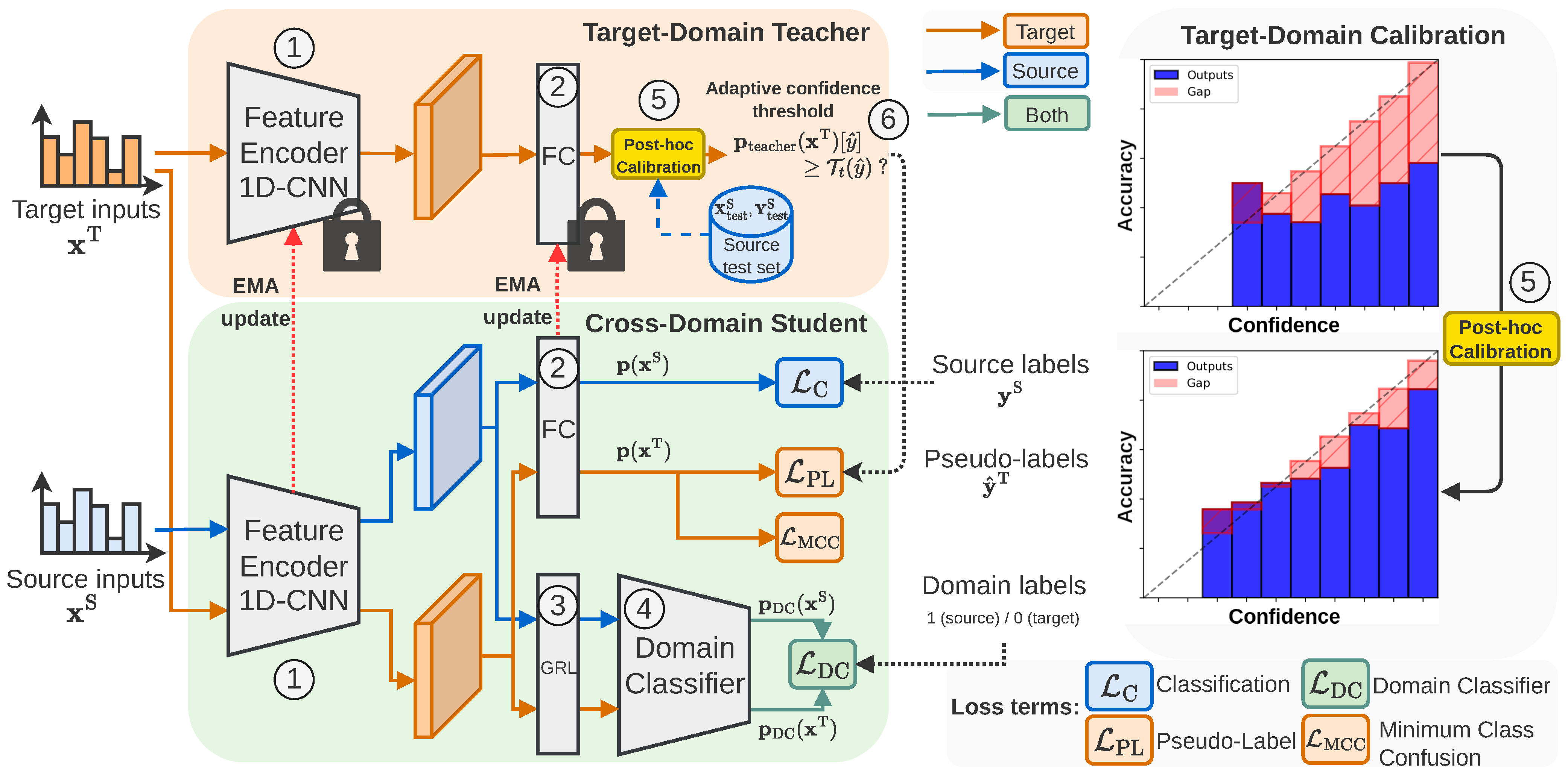
3.1. Overview
3.2. Calibrated Self-Training
3.3. Adaptive Confidence Threshold
3.4. Loss Function and Training Procedure
3.4.1. Student Training
3.4.2. Teacher Updating
3.5. Training Procedure of the Entire Pipeline
| Algorithm 1: Calibrated Adaptive Teacher (CAT) training procedure |
 |
4. Experiments
4.1. Case Study
4.2. Training Parameters
5. Results
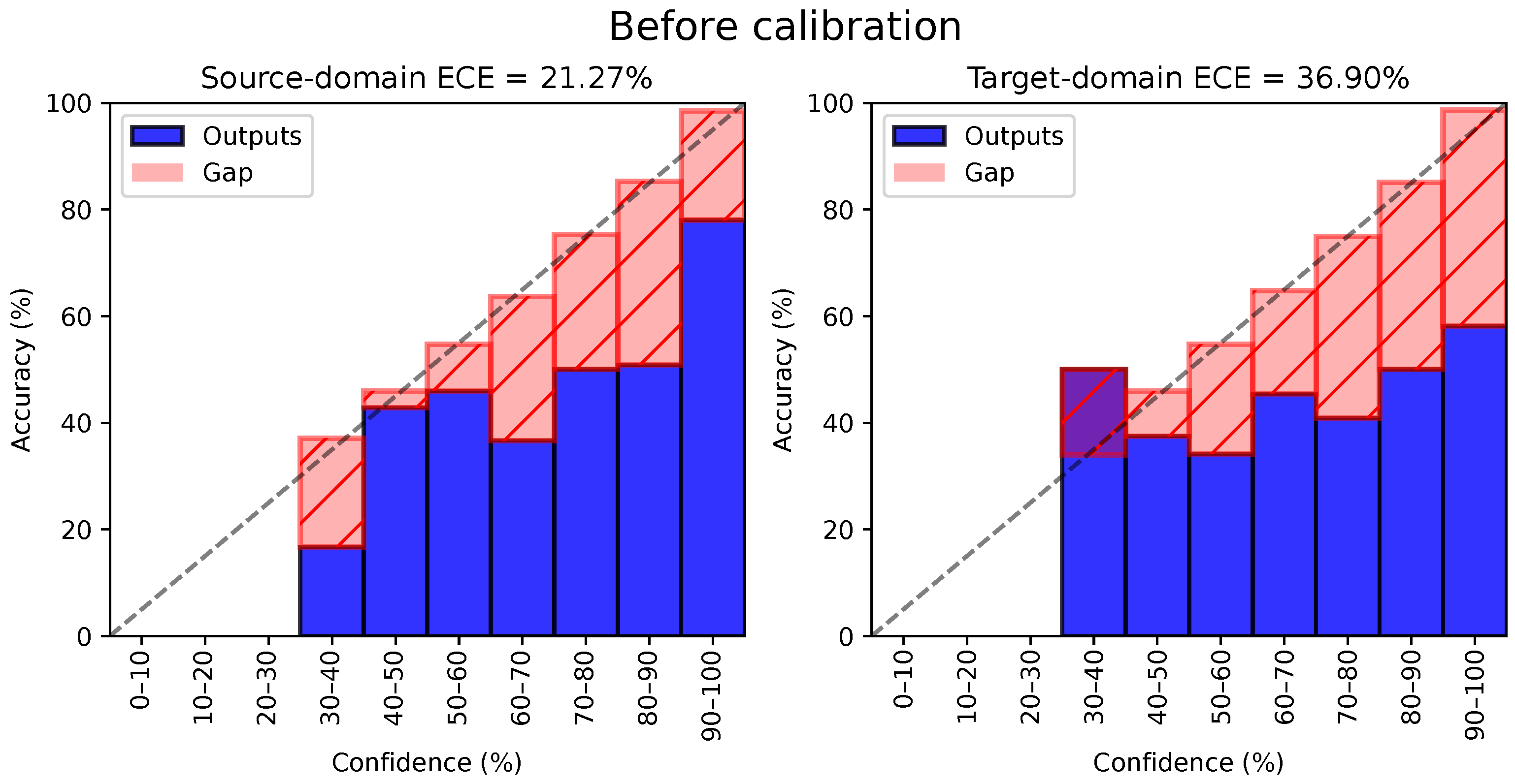
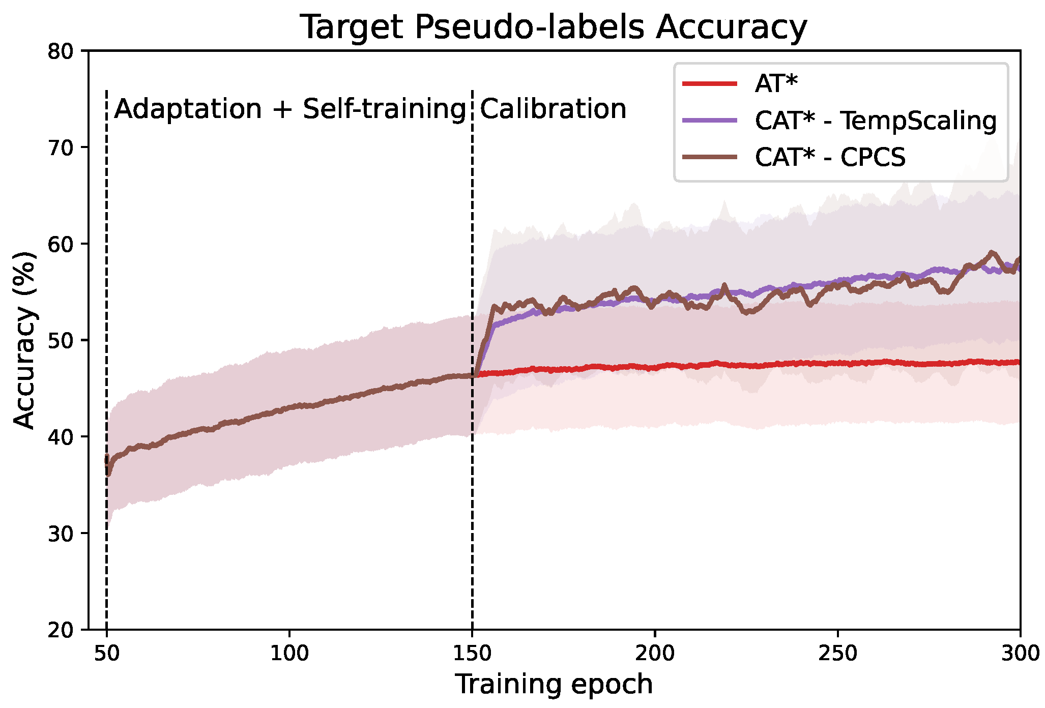
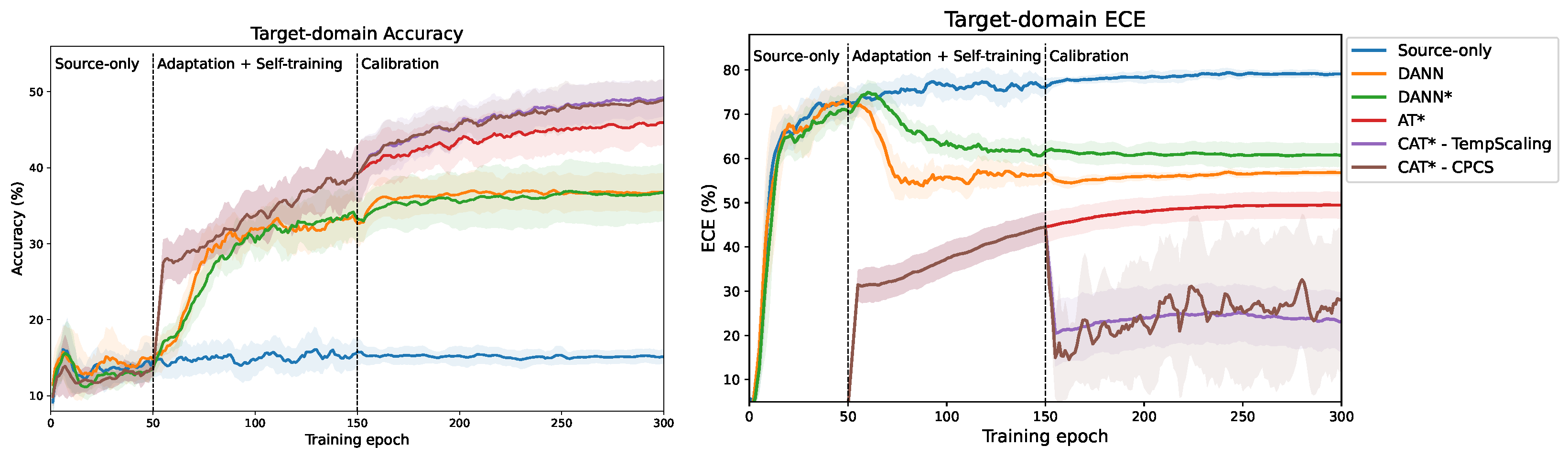
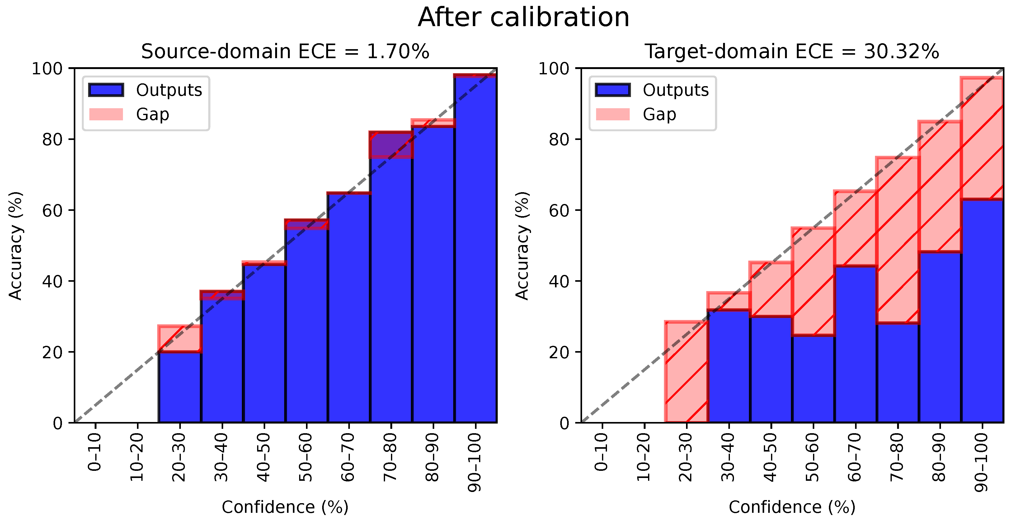
5.1. Calibration and Quality of Pseudo-Labels
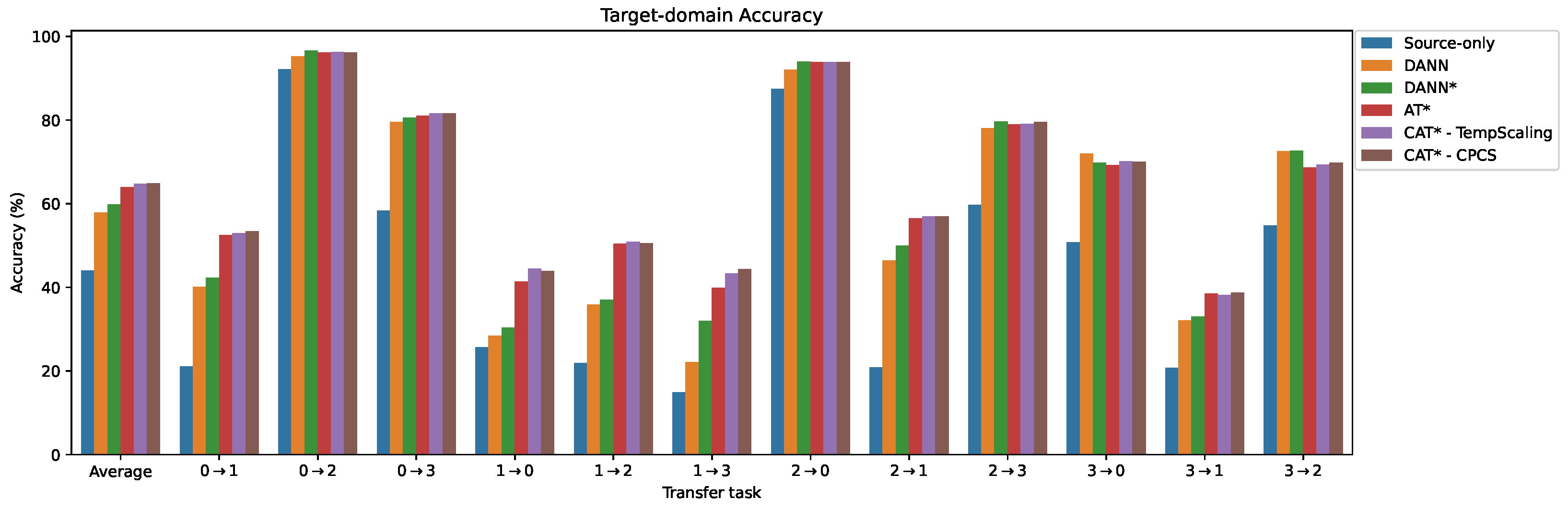
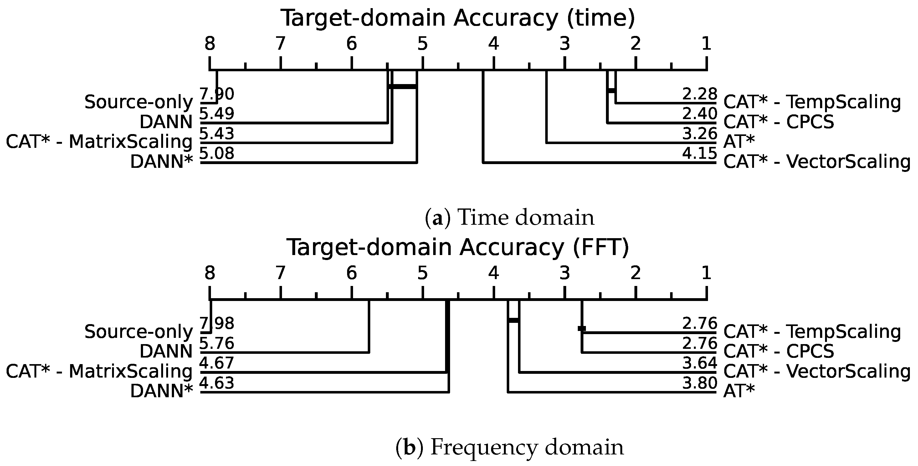
5.2. Comparative Analysis of Performance
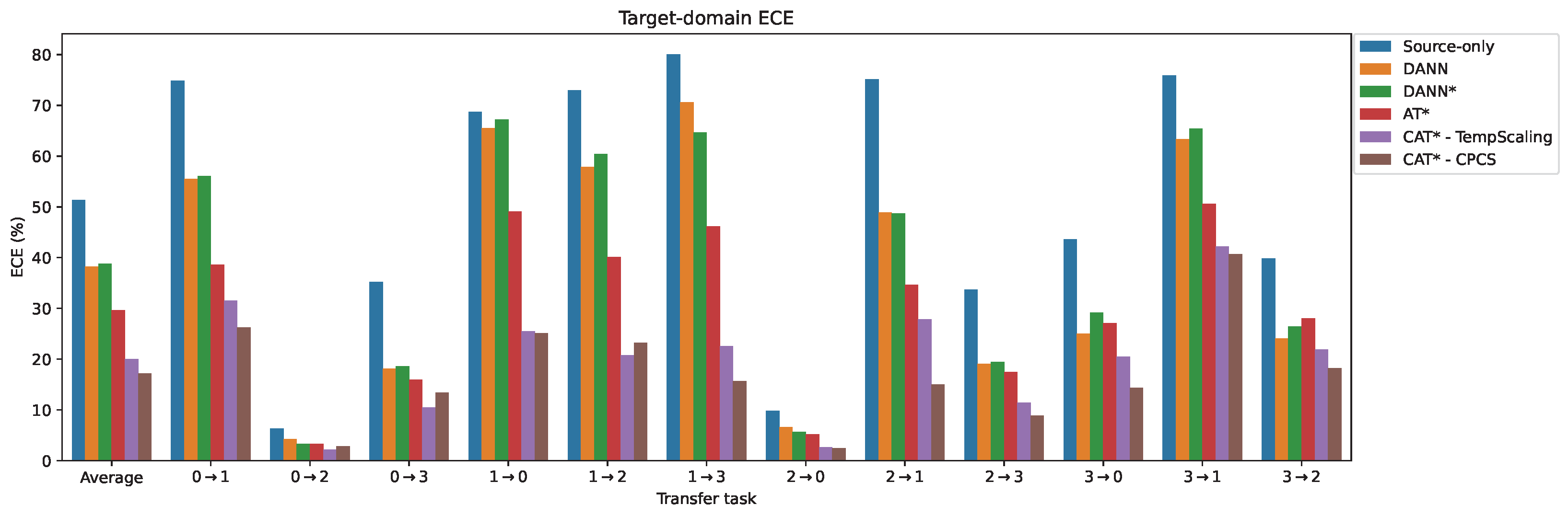
5.3. Comparative Analysis of Calibration Error
5.4. Ablation Studies
6. Conclusions
Author Contributions
Funding
Data Availability Statement
Conflicts of Interest
Abbreviations
| AT | Adaptive Teacher |
| CAT | Calibrated Adaptive Teacher |
| CPCS | Calibrated predictions with covariate shift |
| CPL | Curriculum pseudo-labeling |
| DA | Domain adaptation |
| DANN | Domain-adversarial neural network |
| DC | Domain classifier |
| ECE | Expected calibration error |
| EMA | Exponential moving average |
| FC | Fully connected |
| FFT | Fast Fourier transform |
| GRL | Gradient reversal layer |
| IFD | Intelligent fault diagnosis |
| MCC | Minimum class confusion |
| PU | Paderborn University |
| SDAT | Smooth domain-adversarial training |
| UDA | Unsupervised domain adaptation |
Appendix A. ECE Results for Frequency-Domain Inputs

| Method | Average | Average Rank | ||||||||||||
|---|---|---|---|---|---|---|---|---|---|---|---|---|---|---|
| Source-only | 74.82 | 6.30 | 35.19 | 68.69 | 72.94 | 80.09 | 9.85 | 75.17 | 33.71 | 43.62 | 75.86 | 39.87 | 51.34 | 7.97 |
| DANN | 55.48 | 4.26 | 18.10 | 65.55 | 57.86 | 70.61 | 6.58 | 48.86 | 19.03 | 24.96 | 63.30 | 24.04 | 38.22 | 5.95 |
| DANN* | 56.09 | 3.33 | 18.61 | 67.17 | 60.46 | 64.68 | 5.68 | 48.69 | 19.48 | 29.18 | 65.38 | 26.45 | 38.77 | 6.08 |
| AT* | 38.62 | 3.26 | 15.92 | 49.11 | 40.11 | 46.12 | 5.19 | 34.63 | 17.49 | 27.07 | 50.59 | 28.04 | 29.68 | 4.63 |
| CAT*-TempScaling | 31.54 | 2.20 | 10.50 | 25.46 | 20.76 | 22.53 | 2.60 | 27.88 | 11.39 | 20.49 | 42.23 | 21.90 | 19.96 | 1.78 |
| CAT*-CPCS | 26.27 | 2.78 | 13.38 | 25.11 | 23.21 | 15.61 | 2.43 | 15.01 | 8.88 | 14.32 | 40.67 | 18.16 | 17.15 | 1.82 |
| CAT*-VectorScaling | 39.98 | 2.46 | 13.03 | 32.72 | 28.85 | 29.87 | 3.55 | 35.00 | 14.52 | 23.79 | 51.84 | 23.54 | 24.93 | 3.03 |
| CAT*-MatrixScaling | 42.49 | 4.09 | 16.33 | 39.11 | 32.10 | 35.49 | 5.06 | 41.30 | 18.11 | 27.30 | 53.45 | 25.75 | 28.38 | 4.73 |
References
- Zhao, Z.; Li, T.; Wu, J.; Sun, C.; Wang, S.; Yan, R.; Chen, X. Deep learning algorithms for rotating machinery intelligent diagnosis: An open source benchmark study. ISA Trans. 2020, 107, 224–255. [Google Scholar] [CrossRef] [PubMed]
- Lei, Y.; Yang, B.; Jiang, X.; Jia, F.; Li, N.; Nandi, A.K. Applications of machine learning to machine fault diagnosis: A review and roadmap. Mech. Syst. Signal Process. 2020, 138, 106587. [Google Scholar] [CrossRef]
- Zhao, Z.; Zhang, Q.; Yu, X.; Sun, C.; Wang, S.; Yan, R.; Chen, X. Applications of Unsupervised Deep Transfer Learning to Intelligent Fault Diagnosis: A Survey and Comparative Study. IEEE Trans. Instrum. Meas. 2021, 70, 3525828. [Google Scholar] [CrossRef]
- Li, W.; Huang, R.; Li, J.; Liao, Y.; Chen, Z.; He, G.; Yan, R.; Gryllias, K. A perspective survey on deep transfer learning for fault diagnosis in industrial scenarios: Theories, applications and challenges. Mech. Syst. Signal Process. 2022, 167, 108487. [Google Scholar] [CrossRef]
- Redko, I.; Habrard, A.; Morvant, E.; Sebban, M.; Bennani, Y. Advances in Domain Adaptation Theory; Elsevier: Amsterdam, The Netherlands, 2019. [Google Scholar]
- Wang, Q.; Michau, G.; Fink, O. Domain Adaptive Transfer Learning for Fault Diagnosis. In Proceedings of the 2019 Prognostics and System Health Management Conference (PHM-Paris), Paris, France, 2–5 May 2019; pp. 279–285, ISSN 2166-5656. [Google Scholar] [CrossRef]
- Huang, M.; Yin, J.; Yan, S.; Xue, P. A fault diagnosis method of bearings based on deep transfer learning. Simul. Model. Pract. Theory 2023, 122, 102659. [Google Scholar] [CrossRef]
- Michau, G.; Fink, O. Domain Adaptation for One-Class Classification: Monitoring the Health of Critical Systems Under Limited Information. Int. J. Progn. Health Manag. 2019, 10, 4. [Google Scholar] [CrossRef]
- Shen, F.; Langari, R.; Yan, R. Transfer between multiple machine plants: A modified fast self-organizing feature map and two-order selective ensemble based fault diagnosis strategy. Measurement 2020, 151, 107155. [Google Scholar] [CrossRef]
- Zhu, J.; Chen, N.; Shen, C. A New Multiple Source Domain Adaptation Fault Diagnosis Method Between Different Rotating Machines. IEEE Trans. Ind. Informatics 2021, 17, 4788–4797. [Google Scholar] [CrossRef]
- Nejjar, I.; Geissmann, F.; Zhao, M.; Taal, C.; Fink, O. Domain adaptation via alignment of operation profile for Remaining Useful Lifetime prediction. Reliab. Eng. Syst. Saf. 2024, 242, 109718. [Google Scholar] [CrossRef]
- Yang, B.; Lei, Y.; Jia, F.; Xing, S. An intelligent fault diagnosis approach based on transfer learning from laboratory bearings to locomotive bearings. Mech. Syst. Signal Process. 2019, 122, 692–706. [Google Scholar] [CrossRef]
- Wang, Q.; Taal, C.; Fink, O. Integrating Expert Knowledge with Domain Adaptation for Unsupervised Fault Diagnosis. IEEE Trans. Instrum. Meas. 2022, 71, 3500312. [Google Scholar] [CrossRef]
- Lou, Y.; Kumar, A.; Xiang, J. Machinery Fault Diagnosis Based on Domain Adaptation to Bridge the Gap Between Simulation and Measured Signals. IEEE Trans. Instrum. Meas. 2022, 71, 3180416. [Google Scholar] [CrossRef]
- Long, M.; Cao, Y.; Wang, J.; Jordan, M. Learning Transferable Features with Deep Adaptation Networks. In Proceedings of the 32nd International Conference on Machine Learning, PMLR, Lille, France, 7–9 July 2015; pp. 97–105, ISSN 1938-7228. [Google Scholar]
- Saito, K.; Watanabe, K.; Ushiku, Y.; Harada, T. Maximum Classifier Discrepancy for Unsupervised Domain Adaptation. In Proceedings of the 2018 IEEE/CVF Conference on Computer Vision and Pattern Recognition, Salt Lake City, UT, USA, 18–22 June 2018; pp. 3723–3732. [Google Scholar] [CrossRef]
- Courty, N.; Flamary, R.; Habrard, A.; Rakotomamonjy, A. Joint distribution optimal transportation for domain adaptation. In Proceedings of the Advances in Neural Information Processing Systems, Long Beach, CA, USA, 4–9 December 2017. [Google Scholar]
- Ganin, Y.; Ustinova, E.; Ajakan, H.; Germain, P.; Larochelle, H.; Laviolette, F.; March, M.; Lempitsky, V. Domain-Adversarial Training of Neural Networks. J. Mach. Learn. Res. 2016, 17, 1–35. [Google Scholar]
- Dai, B.; Frusque, G.; Li, T.; Li, Q.; Fink, O. Smart filter aided domain adversarial neural network for fault diagnosis in noisy industrial scenarios. Eng. Appl. Artif. Intell. 2023, 126, 107202. [Google Scholar] [CrossRef]
- Amini, M.R.; Feofanov, V.; Pauletto, L.; Hadjadj, L.; Devijver, E.; Maximov, Y. Self-Training: A Survey. arXiv 2023, arXiv:2202.12040. [Google Scholar] [CrossRef]
- Hao, Y.; Forest, F.; Fink, O. Simplifying Source-Free Domain Adaptation for Object Detection: Effective Self-Training Strategies and Performance Insights. arXiv 2024, arXiv:2407.07586. [Google Scholar]
- Lee, D.H. Pseudo-Label: The Simple and Efficient Semi-Supervised Learning Method for Deep Neural Networks. In Proceedings of the ICML 2013 Workshop: Challenges in Representation Learning (WREPL), Atlanta, GA, USA, 16–21 June 2013. [Google Scholar]
- Blum, A.; Mitchell, T. Combining labeled and unlabeled data with co-training. In Proceedings of the Eleventh Annual Conference on Computational Learning Theory, New York, NY, USA, 24–26 July 1998; COLT’ 98. pp. 92–100. [Google Scholar] [CrossRef]
- Amini, M.R.; Gallinari, P. Semi-supervised logistic regression. In Proceedings of the 15th European Conference on Artificial Intelligence, NLD, Lyon, France, 21–26 July 2002; ECAI’02. pp. 390–394. [Google Scholar]
- Grandvalet, Y.; Bengio, Y. Semi-supervised Learning by Entropy Minimization. In Proceedings of the NIPS, Vancouver, BC, Canada, 5–8 December 2005. [Google Scholar]
- Zhang, B.; Wang, Y.; Hou, W.; Wu, H.; Wang, J.; Okumura, M.; Shinozaki, T. FlexMatch: Boosting Semi-Supervised Learning with Curriculum Pseudo Labeling. In Proceedings of the 35th Conference on Neural Information Processing Systems (NeurIPS 2021), Online, 6–14 December 2021. [Google Scholar] [CrossRef]
- Tur, G.; Hakkani-Tür, D.; Schapire, R.E. Combining active and semi-supervised learning for spoken language understanding. Speech Commun. 2005, 45, 171–186. [Google Scholar] [CrossRef]
- Zhang, W.; Ouyang, W.; Li, W.; Xu, D. Collaborative and Adversarial Network for Unsupervised Domain Adaptation. In Proceedings of the 2018 IEEE/CVF Conference on Computer Vision and Pattern Recognition, Salt Lake City, UT, USA, 18–23 June 2018; pp. 3801–3809, ISSN 2575-7075. [Google Scholar] [CrossRef]
- Zou, Y.; Yu, Z.; Kumar, B.V.K.V.; Wang, J. Domain Adaptation for Semantic Segmentation via Class-Balanced Self-Training. arXiv 2018, arXiv:1810.07911. [Google Scholar] [CrossRef]
- Mei, K.; Zhu, C.; Zou, J.; Zhang, S. Instance Adaptive Self-training for Unsupervised Domain Adaptation. In Proceedings of the Computer Vision—ECCV 2020, Glasgow, UK, 23–28 August 2020; Vedaldi, A., Bischof, H., Brox, T., Frahm, J.M., Eds.; Lecture Notes in Computer Science. Springer: Cham, Switzerland, 2020; pp. 415–430. [Google Scholar] [CrossRef]
- Zheng, Z.; Yang, Y. Rectifying Pseudo Label Learning via Uncertainty Estimation for Domain Adaptive Semantic Segmentation. Int. J. Comput. Vis. 2021, 129, 1106–1120. [Google Scholar] [CrossRef]
- French, G.; Mackiewicz, M.; Fisher, M. Self-ensembling for visual domain adaptation. arXiv 2018, arXiv:1706.05208. [Google Scholar] [CrossRef]
- Odonnat, A.; Feofanov, V.; Redko, I. Leveraging Ensemble Diversity for Robust Self-Training in the Presence of Sample Selection Bias. arXiv 2023, arXiv:2310.14814. [Google Scholar]
- Guo, C.; Pleiss, G.; Sun, Y.; Weinberger, K.Q. On Calibration of Modern Neural Networks. In Proceedings of the 34th International Conference on Machine Learning, PMLR, Sydney, Australia, 6–11 August 2017; pp. 1321–1330, ISSN 2640-3498. [Google Scholar]
- Kuleshov, V.; Fenner, N.; Ermon, S. Accurate Uncertainties for Deep Learning Using Calibrated Regression. In Proceedings of the 35th International Conference on Machine Learning, Stockholm, Sweden, 10–15 July 2018; Volume 80, p. 9. [Google Scholar]
- Deng, X.; Jiang, X. On confidence computation and calibration of deep support vector data description. Eng. Appl. Artif. Intell. 2023, 125, 106646. [Google Scholar] [CrossRef]
- Park, S.; Bastani, O.; Weimer, J.; Lee, I. Calibrated Prediction with Covariate Shift via Unsupervised Domain Adaptation. In Proceedings of the Twenty Third International Conference on Artificial Intelligence and Statistics, PMLR, Online, 26–28 August 2020; pp. 3219–3229, ISSN 2640-3498. [Google Scholar]
- Munir, M.A.; Khan, M.H.; Sarfraz, M.S.; Ali, M. SSAL: Synergizing between Self-Training and Adversarial Learning for Domain Adaptive Object Detection. In Proceedings of the NeurIPS 2021, Online, 6–14 December 2021; p. 13. [Google Scholar]
- Zhang, B.; Li, W.; Hao, J.; Li, X.L.; Zhang, M. Adversarial adaptive 1-D convolutional neural networks for bearing fault diagnosis under varying working condition. arXiv 2018, arXiv:1805.00778. [Google Scholar] [CrossRef]
- She, D.; Peng, N.; Jia, M.; Pecht, M.G. Wasserstein distance based deep multi-feature adversarial transfer diagnosis approach under variable working conditions. J. Instrum. 2020, 15, P06002. [Google Scholar] [CrossRef]
- Li, F.; Tang, T.; Tang, B.; He, Q. Deep convolution domain-adversarial transfer learning for fault diagnosis of rolling bearings. Measurement 2021, 169, 108339. [Google Scholar] [CrossRef]
- Yao, Q.; Qian, Q.; Qin, Y.; Guo, L.; Wu, F. Adversarial domain adaptation network with pseudo-siamese feature extractors for cross-bearing fault transfer diagnosis. Eng. Appl. Artif. Intell. 2022, 113, 104932. [Google Scholar] [CrossRef]
- Wang, X.; Shen, C.; Xia, M.; Wang, D.; Zhu, J.; Zhu, Z. Multi-scale deep intra-class transfer learning for bearing fault diagnosis. Reliab. Eng. Syst. Saf. 2020, 202, 107050. [Google Scholar] [CrossRef]
- Qin, Y.; Qian, Q.; Wang, Z.; Mao, Y. Adaptive manifold partial domain adaptation for fault transfer diagnosis of rotating machinery. Eng. Appl. Artif. Intell. 2023, 126, 107082. [Google Scholar] [CrossRef]
- Jia, S.; Wang, J.; Han, B.; Zhang, G.; Wang, X.; He, J. A Novel Transfer Learning Method for Fault Diagnosis Using Maximum Classifier Discrepancy with Marginal Probability Distribution Adaptation. IEEE Access 2020, 8, 71475–71485. [Google Scholar] [CrossRef]
- Wu, S.; Jing, X.Y.; Zhang, Q.; Wu, F.; Zhao, H.; Dong, Y. Prediction Consistency Guided Convolutional Neural Networks for Cross-Domain Bearing Fault Diagnosis. IEEE Access 2020, 8, 120089–120103. [Google Scholar] [CrossRef]
- Zhu, W.; Shi, B.; Feng, Z. A Transfer Learning Method Using High-quality Pseudo Labels for Bearing Fault Diagnosis. IEEE Trans. Instrum. Meas. 2022, 72, 3502311. [Google Scholar] [CrossRef]
- Gal, Y.; Ghahramani, Z. Dropout as a Bayesian Approximation: Representing Model Uncertainty in Deep Learning. In Proceedings of the 33rd International Conference on Machine Learning, PMLR, New York, NY, USA, 20–22 June 2016; pp. 1050–1059, ISSN 1938-7228. [Google Scholar]
- Wang, J.; Zeng, Z.; Zhang, H.; Barros, A.; Miao, Q. An hybrid domain adaptation diagnostic network guided by curriculum pseudo labels for electro-mechanical actuator. Reliab. Eng. Syst. Saf. 2022, 228, 108770. [Google Scholar] [CrossRef]
- Chen, P.; Zhao, R.; He, T.; Wei, K.; Yuan, J. Unsupervised structure subdomain adaptation based the Contrastive Cluster Center for bearing fault diagnosis. Eng. Appl. Artif. Intell. 2023, 122, 106141. [Google Scholar] [CrossRef]
- Hu, Y.; Baraldi, P.; Di Maio, F.; Zio, E. A Systematic Semi-Supervised Self-adaptable Fault Diagnostics approach in an evolving environment. Mech. Syst. Signal Process. 2017, 88, 413–427. [Google Scholar] [CrossRef]
- Tao, X.; Ren, C.; Li, Q.; Guo, W.; Liu, R.; He, Q.; Zou, J. Bearing defect diagnosis based on semi-supervised kernel Local Fisher Discriminant Analysis using pseudo labels. ISA Trans. 2021, 110, 394–412. [Google Scholar] [CrossRef]
- Zhang, X.; Su, Z.; Hu, X.; Han, Y.; Wang, S. Semisupervised Momentum Prototype Network for Gearbox Fault Diagnosis Under Limited Labeled Samples. IEEE Trans. Ind. Informatics 2022, 18, 6203–6213. [Google Scholar] [CrossRef]
- Long, J.; Chen, Y.; Yang, Z.; Huang, Y.; Li, C. A novel self-training semi-supervised deep learning approach for machinery fault diagnosis. Int. J. Prod. Res. 2022, 61, 8238–8251. [Google Scholar] [CrossRef]
- Li, Y.J.; Dai, X.; Ma, C.Y.; Liu, Y.C.; Chen, K.; Wu, B.; He, Z.; Kitani, K.; Vajda, P. Cross-Domain Adaptive Teacher for Object Detection. In Proceedings of the 2022 IEEE/CVF Conference on Computer Vision and Pattern Recognition (CVPR), New Orleans, LA, USA, 18–24 June 2022; p. 10. [Google Scholar]
- Tarvainen, A.; Valpola, H. Mean teachers are better role models: Weight-averaged consistency targets improve semi-supervised deep learning results. arXiv 2018, arXiv:1703.01780. [Google Scholar] [CrossRef]
- Laine, S.; Aila, T. Temporal Ensembling for Semi-Supervised Learning. arXiv 2017, arXiv:1610.02242. [Google Scholar] [CrossRef]
- Liu, Y.C.; Ma, C.Y.; He, Z.; Kuo, C.W.; Chen, K.; Zhang, P.; Wu, B.; Kira, Z.; Vajda, P. Unbiased Teacher for Semi-Supervised Object Detection. arXiv 2021, arXiv:2102.09480. [Google Scholar] [CrossRef]
- Niculescu-Mizil, A.; Caruana, R. Predicting good probabilities with supervised learning. In Proceedings of the 22nd International Conference on Machine Learning—ICML’05, Bonn, Germany, 7–11 August 2005; pp. 625–632. [Google Scholar] [CrossRef]
- Naeini, M.P.; Cooper, G.F.; Hauskrecht, M. Obtaining Well Calibrated Probabilities Using Bayesian Binning. AAAI Conf. Artif. Intell. 2015, 2015, 2901–2907. [Google Scholar]
- Hebbalaguppe, R.; Prakash, J.; Madan, N.; Arora, C. A Stitch in Time Saves Nine: A Train-Time Regularizing Loss for Improved Neural Network Calibration. In Proceedings of the 2022 IEEE/CVF Conference on Computer Vision and Pattern Recognition (CVPR), New Orleans, LA, USA, 18–24 June 2022; pp. 16060–16069, ISSN 2575-7075. [Google Scholar] [CrossRef]
- Ovadia, Y.; Fertig, E.; Ren, J.; Nado, Z.; Sculley, D.; Nowozin, S.; Dillon, J.V.; Lakshminarayanan, B.; Snoek, J. Can You Trust Your Model’s Uncertainty? Evaluating Predictive Uncertainty Under Dataset Shift. arXiv 2019, arXiv:1906.02530. [Google Scholar] [CrossRef]
- Brier, G.W. Verification of Forecasts Expressed in Terms of Probability. Mon. Weather Rev. 1950, 78, 1–3. [Google Scholar] [CrossRef]
- Rangwani, H.; Aithal, S.K.; Mishra, M.; Jain, A.; Babu, R.V. A Closer Look at Smoothness in Domain Adversarial Training. arXiv 2022, arXiv:2206.08213. [Google Scholar] [CrossRef]
- Foret, P.; Kleiner, A.; Mobahi, H. Sharpness-Aware Minimization for Efficiently Improving Generalization. In Proceedings of the ICLR, Virtual Event, 3–7 May 2021. [Google Scholar]
- Jin, Y.; Wang, X.; Long, M.; Wang, J. Minimum Class Confusion for Versatile Domain Adaptation. In Proceedings of the Computer Vision—ECCV 2020, Glasgow, UK, 23–28 August 2020; Vedaldi, A., Bischof, H., Brox, T., Frahm, J.M., Eds.; Springer: Cham, Switzerland, 2020. Lecture Notes in Computer Science. pp. 464–480. [Google Scholar] [CrossRef]
- Lessmeier, C.; Kimotho, J.K.; Zimmer, D.; Sextro, W. Condition Monitoring of Bearing Damage in Electromechanical Drive Systems by Using Motor Current Signals of Electric Motors: A Benchmark Data Set for Data-Driven Classification. In Proceedings of the European Conference of the Prognostics and Health Management Society, Bilbao, Spain, 5–8 July 2016. [Google Scholar]
- Chen, X.; Yang, R.; Xue, Y.; Huang, M.; Ferrero, R.; Wang, Z. Deep Transfer Learning for Bearing Fault Diagnosis: A Systematic Review Since 2016. IEEE Trans. Instrum. Meas. 2023, 72, 3244237. [Google Scholar] [CrossRef]
- Ruan, D.; Wang, J.; Yan, J.; Gühmann, C. CNN parameter design based on fault signal analysis and its application in bearing fault diagnosis. Adv. Eng. Inform. 2023, 55, 101877. [Google Scholar] [CrossRef]
- Rombach, K.; Michau, G.; Fink, O. Controlled generation of unseen faults for Partial and Open-Partial domain adaptation. Reliab. Eng. Syst. Saf. 2023, 230, 108857. [Google Scholar] [CrossRef]
- Randall, R.B.; Antoni, J. Rolling element bearing diagnostics—A tutorial. Mech. Syst. Signal Process. 2011, 25, 485–520. [Google Scholar] [CrossRef]
- Demsar, J. Statistical Comparisons of Classifiers over Multiple Data Sets. J. Mach. Learn. Res. 2006, 7, 1–30. [Google Scholar]


| Method | Backbone | Time | Frequency | Feature Alignment | Self-Training | Pseudo-Label Filtering | Auxiliary Loss |
|---|---|---|---|---|---|---|---|
| PCG-CNN [46] | 1D-CNN | ✓ | - | MT with consistency loss | Fixed threshold | Class-balance loss | |
| Wang et al. [49] | 1D-CNN | ✓ | DAW | PL | Adaptive threshold | Triplet loss | |
| DTL-IPLL [47] | 1D-CNN | ✓ | MK-MMD | PL | Adaptive threshold + “make decision twice” | - | |
| CAT (ours) | 1D-CNN | ✓ | ✓ | DANN | MT with PL | Adaptive threshold + calibration | - |
| Module | Layers | Parameters | Notation |
|---|---|---|---|
| 1D-CNN backbone | Conv1D, BatchNorm, ReLU | in = 1, out = 16, kernel = 15 | |
| Conv1D, BatchNorm, ReLU | in = 16, out = 32, kernel = 3 | ||
| MaxPool1D | kernel = 2, stride = 2 | ||
| Conv1D, BatchNorm, ReLU | in = 32, out = 64, kernel = 3 | ||
| Conv1D, BatchNorm, ReLU | in = 64, out = 128, kernel = 3 | ||
| AdaptiveMaxPool1D | out = 128 × 4 | ||
| FC, ReLU | in = 128 × 4, out = 256 | ||
| Dropout | p = 0.5 | ||
| Bottleneck | FC, ReLU | in = 256, out = 256 | |
| Dropout | p = 0.5 | ||
| Classification head | FC, Softmax | in = 256, out = 13 | |
| Domain classifier | FC, ReLU | in = 256, out = 1024 | |
| Dropout | p = 0.5 | ||
| FC, ReLU | in = 1024, out = 1024 | ||
| Dropout | p = 0.5 | ||
| FC, Sigmoid | in = 1024, out = 1 |
| Domain | Rotational Speed | Load Torque | Radial Force |
|---|---|---|---|
| 0 | 1500 rpm | 0.7 Nm | 1000 N |
| 1 | 900 rpm | 0.7 Nm | 1000 N |
| 2 | 1500 rpm | 0.1 Nm | 1000 N |
| 3 | 1500 rpm | 0.7 Nm | 400 N |
| Class | Bearing Code | Damage | Element | Combination | Characteristic |
|---|---|---|---|---|---|
| 0 | KA04 | Fatigue: pitting | OR | S | Single point |
| 1 | KA15 | Plastic deform: indentations | OR | S | Single point |
| 2 | KA16 | Fatigue: pitting | OR | R | Single point |
| 3 | KA22 | Fatigue: pitting | OR | S | Single point |
| 4 | KA30 | Plastic deform: indentations | OR | R | Distributed |
| 5 | KB23 | Fatigue: pitting | IR (+OR) | M | Single point |
| 6 | KB24 | Fatigue: pitting | IR (+OR) | M | Distributed |
| 7 | KB27 | Plastic deform: indentations | OR+IR | M | Distributed |
| 8 | KI14 | Fatigue: pitting | IR | M | Single point |
| 9 | KI16 | Fatigue: pitting | IR | S | Single point |
| 10 | KI17 | Fatigue: pitting | IR | R | Single point |
| 11 | KI18 | Fatigue: pitting | IR | S | Single point |
| 12 | KI21 | Fatigue: pitting | IR | S | Single point |
| Method | Average | Average Rank | ||||||||||||
|---|---|---|---|---|---|---|---|---|---|---|---|---|---|---|
| Source-only † | 14.02 | 76.33 | 30.02 | 23.57 | 24.18 | 16.09 | 76.73 | 14.71 | 31.23 | 32.16 | 25.27 | 32.39 | 33.06 | - |
| DANN † | 38.19 | 79.97 | 53.74 | 35.42 | 39.57 | 27.05 | 79.20 | 36.53 | 49.23 | 47.93 | 27.45 | 47.57 | 46.82 | - |
| Source-only | 15.15 | 78.23 | 30.29 | 24.33 | 25.71 | 17.73 | 76.41 | 13.87 | 33.34 | 31.92 | 26.32 | 32.12 | 33.78 | 7.90 |
| DANN | 36.96 | 81.22 | 51.56 | 35.55 | 40.89 | 28.35 | 78.77 | 33.83 | 47.29 | 47.56 | 29.94 | 46.41 | 46.53 | 5.49 |
| DANN* | 36.53 | 83.54 | 54.46 | 35.61 | 38.53 | 25.75 | 81.44 | 36.53 | 49.86 | 47.25 | 28.50 | 46.20 | 47.02 | 5.08 |
| AT* | 49.36 | 82.17 | 56.16 | 47.83 | 50.66 | 34.92 | 81.72 | 49.11 | 51.80 | 50.08 | 29.91 | 53.86 | 53.13 | 3.26 |
| CAT*-TempScaling | 52.67 | 82.44 | 57.00 | 51.27 | 53.34 | 36.34 | 81.78 | 51.44 | 54.40 | 49.22 | 30.37 | 53.74 | 54.50 | 2.28 |
| CAT*-CPCS | 52.42 | 82.29 | 57.25 | 51.24 | 52.76 | 36.46 | 81.69 | 51.63 | 54.25 | 49.40 | 29.88 | 53.77 | 54.42 | 2.40 |
| CAT*-VectorScaling | 34.51 | 82.08 | 50.95 | 43.66 | 45.53 | 34.10 | 82.03 | 40.18 | 48.35 | 47.99 | 35.92 | 46.75 | 49.34 | 4.15 |
| CAT*-MatrixScaling | 33.65 | 82.08 | 48.20 | 39.97 | 44.58 | 32.04 | 80.95 | 35.37 | 46.14 | 44.73 | 31.01 | 43.48 | 46.85 | 5.43 |
| Method | Average | Average Rank | ||||||||||||
|---|---|---|---|---|---|---|---|---|---|---|---|---|---|---|
| Source-only † | 20.96 | 90.87 | 57.14 | 25.13 | 24.14 | 13.75 | 86.40 | 20.55 | 57.18 | 52.58 | 20.90 | 53.64 | 43.60 | - |
| DANN † | 40.34 | 93.71 | 82.15 | 28.48 | 35.27 | 22.88 | 92.50 | 46.01 | 79.52 | 68.76 | 24.57 | 76.15 | 57.53 | - |
| Source-only | 21.13 | 92.12 | 58.34 | 25.68 | 21.92 | 14.92 | 87.47 | 20.83 | 59.76 | 50.81 | 20.71 | 54.75 | 44.04 | 7.98 |
| DANN | 40.09 | 95.27 | 79.58 | 28.45 | 35.88 | 22.15 | 92.07 | 46.44 | 78.03 | 71.98 | 32.09 | 72.61 | 57.89 | 5.76 |
| DANN* | 42.30 | 96.58 | 80.64 | 30.41 | 37.07 | 31.98 | 93.98 | 50.00 | 79.64 | 69.83 | 32.98 | 72.73 | 59.84 | 4.63 |
| AT* | 52.55 | 96.12 | 81.09 | 41.41 | 50.44 | 39.85 | 93.86 | 56.50 | 79.03 | 69.28 | 38.53 | 68.64 | 63.94 | 3.80 |
| CAT*-TempScaling | 52.98 | 96.27 | 81.57 | 44.45 | 50.87 | 43.36 | 93.89 | 56.99 | 79.06 | 70.11 | 38.22 | 69.34 | 64.76 | 2.76 |
| CAT*-CPCS | 53.47 | 96.18 | 81.60 | 43.96 | 50.60 | 44.33 | 93.89 | 56.93 | 79.58 | 70.05 | 38.71 | 69.77 | 64.92 | 2.76 |
| CAT*-VectorScaling | 50.92 | 96.40 | 81.24 | 43.53 | 48.40 | 41.97 | 94.10 | 55.18 | 78.61 | 69.25 | 37.55 | 69.50 | 63.89 | 3.64 |
| CAT*-MatrixScaling | 49.97 | 95.82 | 80.85 | 41.41 | 47.57 | 36.85 | 93.98 | 52.64 | 77.94 | 68.73 | 37.55 | 69.28 | 62.72 | 4.67 |
| Method | Average | Average Rank | ||||||||||||
|---|---|---|---|---|---|---|---|---|---|---|---|---|---|---|
| Source-only | 78.90 | 17.41 | 62.44 | 66.60 | 66.11 | 74.27 | 18.24 | 79.20 | 58.15 | 56.86 | 62.86 | 57.16 | 58.18 | 7.85 |
| DANN | 55.70 | 14.80 | 41.80 | 55.41 | 49.55 | 62.51 | 16.29 | 57.58 | 45.81 | 43.55 | 59.98 | 45.25 | 45.69 | 6.13 |
| DANN* | 60.17 | 14.81 | 42.89 | 59.57 | 56.73 | 68.97 | 16.86 | 59.73 | 47.24 | 48.83 | 66.33 | 49.83 | 49.33 | 6.88 |
| AT* | 41.51 | 12.60 | 34.33 | 38.96 | 37.04 | 48.46 | 12.90 | 38.07 | 37.27 | 32.34 | 49.30 | 28.29 | 34.26 | 4.15 |
| CAT*-TempScaling | 14.16 | 3.95 | 12.30 | 6.64 | 9.54 | 18.10 | 6.24 | 15.49 | 15.84 | 14.39 | 27.75 | 8.87 | 12.77 | 1.67 |
| CAT*-CPCS | 21.09 | 6.36 | 10.76 | 8.34 | 6.77 | 19.28 | 4.89 | 12.44 | 11.63 | 6.94 | 17.19 | 10.05 | 11.31 | 1.48 |
| CAT*-VectorScaling | 49.19 | 5.65 | 31.14 | 26.67 | 25.55 | 31.05 | 7.48 | 44.31 | 35.41 | 34.69 | 38.83 | 37.78 | 30.65 | 3.35 |
| CAT*-MatrixScaling | 54.38 | 8.03 | 36.62 | 27.25 | 25.97 | 32.55 | 11.29 | 48.81 | 41.30 | 39.78 | 47.16 | 42.60 | 34.64 | 4.48 |
| Method | Threshold | Average | ||||||||||||
|---|---|---|---|---|---|---|---|---|---|---|---|---|---|---|
| AT | Fixed | 33.44 | 80.95 | 49.53 | 40.98 | 39.39 | 23.00 | 79.75 | 36.60 | 44.21 | 50.23 | 29.20 | 47.33 | 46.22 |
| AT | Adaptive | 38.77 | 80.89 | 52.50 | 41.63 | 44.34 | 26.29 | 78.86 | 42.88 | 45.90 | 49.03 | 28.99 | 51.21 | 48.33 |
| Method | MCC | SDAT | Average | ||||||||||||
|---|---|---|---|---|---|---|---|---|---|---|---|---|---|---|---|
| AT | 38.77 | 80.89 | 52.50 | 41.63 | 44.34 | 26.29 | 78.86 | 42.88 | 45.90 | 49.03 | 28.99 | 51.21 | 48.33 | ||
| ✓ | 42.77 | 80.92 | 52.89 | 43.53 | 46.75 | 28.38 | 80.83 | 43.87 | 46.44 | 51.34 | 32.73 | 51.45 | 50.04 | ||
| ✓ | 45.98 | 82.32 | 54.98 | 45.28 | 46.41 | 30.89 | 81.04 | 48.71 | 50.80 | 44.18 | 26.44 | 50.05 | 50.59 | ||
| ✓ | ✓ | 49.36 | 82.17 | 56.16 | 47.83 | 50.66 | 34.92 | 81.72 | 49.11 | 51.80 | 50.08 | 29.91 | 53.86 | 53.13 | |
| CAT - TempScaling | 44.58 | 81.40 | 53.95 | 47.04 | 46.99 | 27.87 | 78.92 | 44.82 | 48.14 | 49.59 | 28.99 | 52.18 | 50.28 | ||
| ✓ | 46.56 | 81.34 | 55.16 | 48.91 | 50.14 | 32.44 | 81.17 | 46.38 | 48.35 | 50.60 | 33.22 | 53.07 | 52.28 | ||
| ✓ | 49.14 | 82.41 | 56.58 | 47.50 | 49.92 | 32.47 | 81.01 | 50.00 | 52.34 | 44.70 | 23.19 | 50.14 | 51.62 | ||
| ✓ | ✓ | 52.67 | 82.44 | 57.00 | 51.27 | 53.34 | 36.34 | 81.78 | 51.44 | 54.40 | 49.22 | 30.37 | 53.74 | 54.50 | |
| CAT - CPCS | 43.90 | 81.53 | 53.86 | 46.18 | 46.44 | 27.35 | 79.17 | 44.29 | 48.53 | 49.62 | 30.15 | 52.40 | 50.28 | ||
| ✓ | 46.87 | 81.34 | 54.89 | 48.82 | 50.38 | 32.95 | 81.17 | 46.78 | 48.59 | 51.58 | 33.28 | 52.89 | 52.46 | ||
| ✓ | 49.82 | 82.38 | 57.19 | 47.37 | 49.65 | 30.98 | 81.01 | 51.23 | 52.68 | 45.19 | 23.40 | 49.71 | 51.72 | ||
| ✓ | ✓ | 52.42 | 82.29 | 57.25 | 51.24 | 52.76 | 36.46 | 81.69 | 51.63 | 54.25 | 49.40 | 29.88 | 53.77 | 54.42 |
Disclaimer/Publisher’s Note: The statements, opinions and data contained in all publications are solely those of the individual author(s) and contributor(s) and not of MDPI and/or the editor(s). MDPI and/or the editor(s) disclaim responsibility for any injury to people or property resulting from any ideas, methods, instructions or products referred to in the content. |
© 2024 by the authors. Licensee MDPI, Basel, Switzerland. This article is an open access article distributed under the terms and conditions of the Creative Commons Attribution (CC BY) license (https://creativecommons.org/licenses/by/4.0/).
Share and Cite
Forest, F.; Fink, O. Calibrated Adaptive Teacher for Domain-Adaptive Intelligent Fault Diagnosis. Sensors 2024, 24, 7539. https://doi.org/10.3390/s24237539
Forest F, Fink O. Calibrated Adaptive Teacher for Domain-Adaptive Intelligent Fault Diagnosis. Sensors. 2024; 24(23):7539. https://doi.org/10.3390/s24237539
Chicago/Turabian StyleForest, Florent, and Olga Fink. 2024. "Calibrated Adaptive Teacher for Domain-Adaptive Intelligent Fault Diagnosis" Sensors 24, no. 23: 7539. https://doi.org/10.3390/s24237539
APA StyleForest, F., & Fink, O. (2024). Calibrated Adaptive Teacher for Domain-Adaptive Intelligent Fault Diagnosis. Sensors, 24(23), 7539. https://doi.org/10.3390/s24237539