Abstract
Global warming is influenced by an increase in greenhouse gas (GHG) concentration in the atmosphere. Consequently, Net Ecosystem Exchange (NEE) is the main factor that influences the exchange of carbon (C) between the atmosphere and the soil. As a result, agricultural ecosystems are a potential carbon dioxide (CO2) sink, particularly rice paddies (Oryza sativa). Therefore, a static chamber with a portable CO2 analyzer was designed and implemented for three rice plots to monitor CO2 emissions. Furthermore, a weather station was installed to record meteorological variables. The vegetative, reproductive, and maturation phases of the crop lasted 95, 35, and 42 days post-sowing (DPS), respectively. In total, the crop lasted 172 DPS. Diurnal NEE had the highest CO2 absorption capacity at 10:00 a.m. for the tillering stage (82 and 89 DPS), floral primordium (102 DPS), panicle initiation (111 DPS), and flowering (126 DPS). On the other hand, the maximum CO2 emission at 82, 111, and 126 DPS occurred at 6:00 p.m. At 89 and 102 DPS, it occurred at 4:00 and 6:00 a.m., respectively. NEE in the vegetative stage was −25 , and in the reproductive stage, it was −35 , indicating the highest absorption capacity of the plots. The seasonal dynamics of NEE were mainly controlled by the air temperature inside the chamber (Tc) (R = −0.69), the relative humidity inside the chamber (RHc) (R = −0.66), and net radiation (Rn) (R = −0.75). These results are similar to previous studies obtained via chromatographic analysis and eddy covariance (EC), which suggests that the portable analyzer could be an alternative for CO2 monitoring.
1. Introduction
The increase in the concentration of carbon dioxide (CO2) in the atmosphere is one of the main factors responsible for global warming. Currently, CO2 levels are at 419 ; this represents 150% of the values in the 18th century [1]. This increase is mainly due to anthropogenic activities such as intensive agriculture and changes in land use, among others [2]. Rice (Oryza sativa) cultivation extends from tropical to temperate regions [3]. It is the second most important staple food in the world, with an annual production of 740 Mt [4]. It covers 114 countries and an area of 153 in total, or 11% of the world’s arable land [5]. In 2021, Peru produced 3.5 of rice in an area of 417,000 [6]. Currently, 90% of rice production is obtained through flood irrigation [7], making it a significant source of methane (CH4). Furthermore, nitrous oxide (N2O) is mainly generated by nitrification and denitrification processes, which are closely related to soil moisture [8]. Both gases represent approximately 30% and 11%, respectively, of global agricultural emissions [9].
Net Ecosystem Exchange (NEE) is one of the main processes that influence CO2 concentration in the atmosphere. Agricultural ecosystems, particularly rice paddies, play a crucial role in carbon absorption. Therefore, it is important to understand their function in carbon (C) flux [10]. For example, Chatterjee et al. [11] monitored lowland paddy fields for one year (dry and wet seasons) using eddy covariance (EC) to evaluate variations in NEE and find a suitable model for the better partitioning of NEE with respect to its components, such as gross primary production (GPP) and ecosystem respiration (Reco). Kumar et al. [12] calculated NEE in rice and wheat systems in the northwest Indo-Gangetic plains. This was the first estimation in a rice–wheat spring sequence using EC. Neogi et al. [13] investigated the characterization of CO2 fluxes in tropical lowland rice paddy ecosystems using EC to better understand the environmental impact in terms of C budget in submerged soil.
The land–atmosphere exchange of matter and energy is recorded using EC [14], widely used given its solid theoretical basis. However, it is expensive, difficult to manipulate [15], and susceptible to information gaps [16]. On the other hand, static chambers are used to complement the deficiencies of EC. Nevertheless, they require long monitoring periods [17]. Additionally, the cost of chromatographic analysis for collected gases is high. In this regard, infrared sensors represent an opportunity to solve these challenges. They utilize the non-dispersive infrared (NDIR) principle to measure the concentration of CO2 instantly [18]. In addition, they are easy to acquire, manipulate, and program. An automatic estimation and sampling method based on sensors that can replace the conventional methods mentioned and simultaneously increase the efficiency in estimating greenhouse gas (GHG) fluxes is necessary [19].
In this research, a CO2 analyzer was designed together with a static chamber to monitor diurnal and nocturnal NEE in rice fields. The objective was to establish a novel, efficient, and dependable method of making resource management decisions for sustainable agricultural practices in Peru.
2. Materials and Methods
2.1. Site Description
This research was carried out in the “Experimental Irrigation Area” (AER) on the campus of the National Agrarian University La Molina (UNALM), La Molina District, Lima Province, Lima Region (12°04′41″ S, 76°56′45″ W, altitude: 246 ) (Figure 1). During the study, the maximum, minimum, and average temperatures were 32.3, 15.6, and 23.24 °C, respectively. The maximum precipitation was 2.6 with an average relative humidity of 77%. The meteorological data were recorded using the automatic station VANTAGE Pro2 Davis, Hayward, CA, USA, located at the AER (Figure 2). In addition, the physicochemical characteristics of the soil are detailed in Table 1.
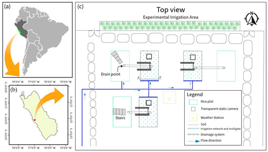
Figure 1.
(a,b) Location of the study area in Lima, Peru. (c) AER map.
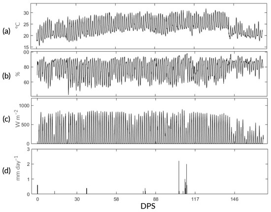
Figure 2.
Predominant climatic conditions during the study. (a–d) Air temperature (Ta), relative humidity (RH), net radiation (Rn), and precipitation (pp).

Table 1.
Physicochemical characteristics of the soil in the study area.
2.2. Design of Portable Analyzer for CO2 Monitoring
A portable analyzer was designed for CO2 monitoring (Figure 3a). Its components are as follows: (a) MHZ19B CO2 sensor from Winsen Electronics; its detection range is 0 to 5000 ± 50 . It operates at optimal Ta and RH conditions of 0 to 50 °C and 0 to 90%, respectively. (b) DHT22 Ta and RH sensor from Aosong Electronics. Its measurement range for Ta is −40 to 80 ± 0.5 °C, and for RH, it is 0 to 100 ± 2%. (c) Real-time clock (RTC) module “DS3231” from MMJ Smart Electronics. (d) microSD memory module from Deeoee Electronics. (e) 16 × 2 LED display from Yuxian Electronics. The Arduino DUE board (g) and “Arduino IDE”, both from Arduino CC, were selected as the microcontroller unit and coding system, respectively. The components were soldered onto a multipurpose board (f) to ensure connection with the ARDUINO board. Then, the system was placed in a plastic box measuring 150 × 110 × 80 . The device was powered by a PHILLIPS 4000 portable battery with 5 of output. The operational analyzer is shown in Figure 3b.
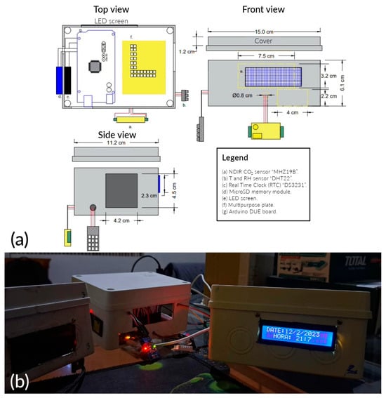
Figure 3.
(a) Scheme of the portable analyzer for CO2 monitoring; (b) analyzer finished.
2.3. Static Transparent Chamber Design
The monitoring system consisted of a static chamber and a portable CO2 analyzer (Figure 4a). The chamber is made of transparent 2 thick transparent acrylic, whose dimensions are 1 × 0.5 × 0.5 . The gas-mixing system consisted of a portable battery (e) and 2 fans (f), both connected through a Universal Serial Bus (USB) port (g). In addition, the metal base, with dimensions of 0.5 × 0.5 × 0.15 , has a 2 thick slot. This was installed 6 below the soil surface before transplanting permanently. In addition, the analyzer is attached to one of the side faces using a support (h). The finished device is shown in Figure 4b.
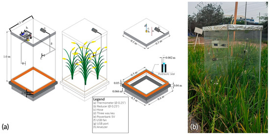
Figure 4.
Transparent static chamber: (a) scheme; (b) disposition.
2.4. Field Management
Three ponds of 3 × 4 × 0.6 were installed and lined with geomembrane (Figure 5a,b). The seedbed was prepared on 11 November 2022 and transplanted 35 days post-sowing (). The distribution was five rice seedlings per hill, spaced 20 × 20 each. The vegetative, reproductive, and maturation phases lasted 95, 35, and 42 , respectively. In total, the crop lasted 172 (Figure 5c). The water regime maintained soil moisture between saturation and a 5 depth. Irrigation water came from the Rimac River and was stored in a 25 tank. Its physicochemical characteristics are described in Table 2. The NPK fertilization dose was 230-60-90. In total, 100% of P and K and 50% of N were applied during transplanting. The remaining N was distributed during tillering, floral primordium, and flowering (Figure 5d). The nitrogen sources were urea, diammonium phosphate (DAP), and “Basacote plus 3M”.
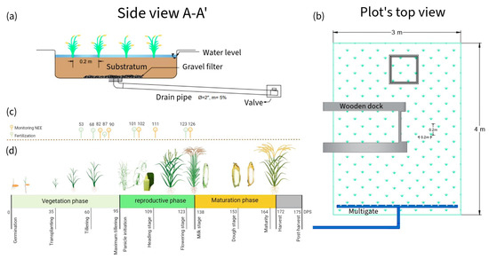
Figure 5.
(a,b) Rice plot’s side and top view, respectively (c) Calendar of monitoring and fertilization days (in DPS); (d) stages of rice paddy growth.
Table 2.
Physicochemical characteristics of water.
2.5. Sensor Calibration
The MHZ19B sensor was calibrated with an automatic reference of 400 by the manufacturer [20]. The DHT22 sensor was calibrated by relating its readings to the hourly data obtained by the automatic weather station for 24 h (Figure 6).
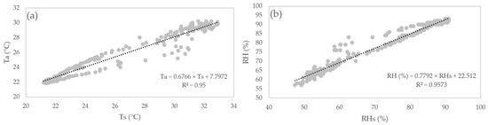
Figure 6.
Correlation graph between the DHT22 sensor and the automatic station. (a) Ta; (b) RH.
Ta is air temperature, Ts is the air temperature reading by the sensor, RH is relative humidity, and RHs is the relative humidity reading by the sensor.
2.6. Monitoring and Data Collection
Diurnal CO2 monitoring in rice plots begins at tillering, the stage of maximum leaf growth. There were 5 days that lasted 24 h each and were carried out simultaneously in the three plots. The preparatory phase began with the attachment of the static camera to the metal base. Then, a water seal was made on the coupling to prevent gas leakage. The analyzer was then placed and turned on in the chamber so that the CO2, Ta, and RH readings stabilized for 30 min. Monitoring per se began with closing the chamber and turning on the fans during the first 30 min of each hour. The opposite action was carried out during the remaining 30 min.
2.7. Data Processing
Emission fluxes were calculated based on CO2 concentration changes . Firstly, linear regression analysis was performed on 30 data [21,22]. Secondly, the CO2 emission flux was calculated with Equations (1)–(3).
where K is the accumulation factor of the chamber ; S is the rate of change in CO2 concentration ; P is barometric pressure ; R is the ideal gas constant, 0.0831451 ; Tc is the temperature inside the chamber (); V is the net volume of the chamber ; and A is the net area of the chamber entrance .
Thirdly, the Michaelis–Menten rectangular hyperbola model was used to calculate NEE [23]. The equation used was (4).
where NEE is the net CO2 flux of the rice ecosystem , PPFD is the photosynthetic photon flux density , Pmax is the maximum photosynthetic rate, Km is an adjustment constant, and Reco is the respiration rate of the rice ecosystems . For this, PPFD, Pmax, and Km data from Yang et al. [21] were used. The daily NEE for each phenological stage is the average of the fluxes from three analyzers. To verify the normality of the data, the Anderson–Darling test was used, which turned out to be non-parametric. Spearman correlation () was performed between the environmental variables, NEE, and Reco. Additionally, the Mann–Whitney U test was applied to assess significant differences between the results, at a significance level of 5%.
3. Results
3.1. Diurnal Variations in NEE
Figure 7 shows the diurnal behavior of NEE in the rice plots. The positive and negative signs indicate the net emission and absorption of CO2, respectively. The maximum CO2 emission at 89 and 102 DPS was at 4:00 and 6:00 a.m., whose values are 0.361 and 0.318 . At 82, 111, and 126 DPS, it was at 18:00 with values of 0.68, 1, and 0.22 . On the other hand, the maximum CO2 assimilation occurred at 10:00 a.m., with values of −9.51, −9.25, −13.63, −12.9, and −12.5 for 82, 89, 102, 111, and 126 DPS, respectively.
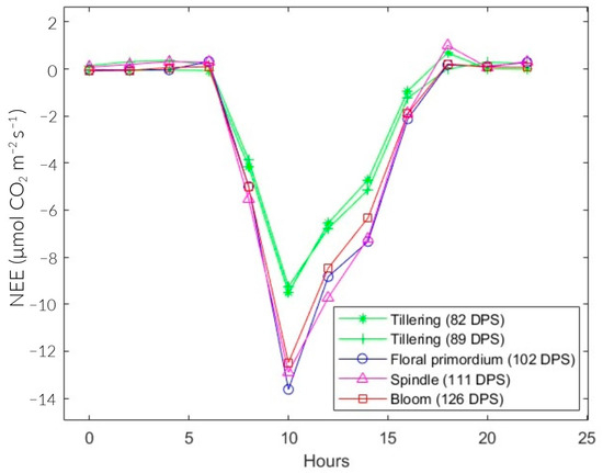
Figure 7.
Diurnal NEE for different growth stages of rice fields.
The total NEE was higher during the tillering stage on average (82 and 89 DPS), with −25.07 on average. In floral primordium (102 DPS), it reached the minimum at −36.14 . Then, it progressively increased during the spindle stage (111 DPS) at −34.98 and the flowering stage (126 DPS) at −33.83 . Likewise, the seasonal variations in NEE in the vegetative and reproductive phases were −25.07 and −34.98 , respectively (Table 3).
Table 3.
Diurnal NEE (µmolCO2 m2 s−1) for different growth stages in rice fields.
3.2. NEE Response to Environmental Factors
The results of the Anderson–Darling test verified the non-normality of the data, except for Ts. Then, the correlations between the environmental factors, Reco, and NEE were analyzed. Coefficients close to 1 and −1 indicate strong positive and negative correlations, respectively (Figure 8). NEE was positively and significantly correlated with RHc (R = 0.66, p < 0.05) and Ts (R = 0.26, p < 0.05). Furthermore, it showed a highly significant negative correlation with Rn (R = −0.75, p < 0.05) and Tc (R = −0.69, p < 0.05). On the other hand, Reco was highly positively associated with Tc (R = 0.7, p < 0.05) and Rn (R = 0.73, p < 0.05). In addition, it showed a significant negative correlation with RHc (R = −0.55, p < 0.05) and Ts (R = −0.4, p < 0.05).
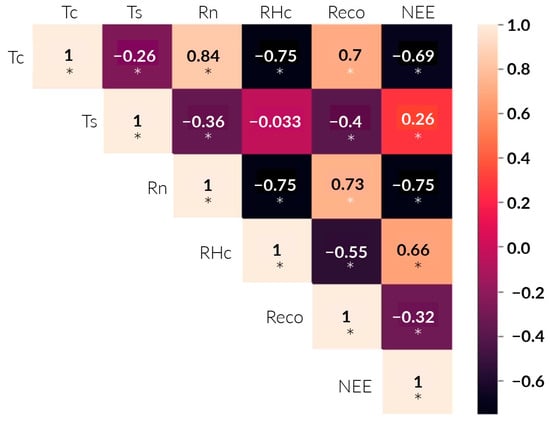
Figure 8.
Spearman correlation heat map (R) between NEE, Reco, and environmental variables. Light and dark colors indicate positive and negative correlations, respectively. “*” indicates a significant correlation at the 0.05 level (p < 0.05).
4. Discussion
4.1. Diurnal Variation in NEE
The NEE values during the study are represented in Figure 7. They are positive at night and negative during the day. This behavior is consistent with the results obtained by Bhattacharyya et al. [24], McMillan et al. [25], and Zhang et al. [26]. During daylight hours, the ecosystem functioned as a carbon dioxide (CO2) sink, with higher levels of absorption through photosynthesis compared with emissions through respiratory processes. However, during the nighttime, the ecosystem acted as a source of CO2, primarily because of Reco [27,28]. In the absence of sunlight, NEE is, on average, 58 times lower than the results of Yang et al. [21] and Bhattacharyya et al. [29]. This decrease can be attributed to the higher levels of RHc during the same period (Figure 9d). As a result, the sensor did not perform at its optimal level. In contrast to portable analyzer technology, the EC methodology used in the aforementioned studies employed open-path NDIR gas analyzers such as the LI-7200, LI-7500, and EC-150. These are specifically designed to measure fluxes in CO2, water vapor, and energy below the canopy. Therefore, their prices are excessively higher compare with a portable analyzer. In this study, the “MHZ19B” NDIR sensor was used, which differs in application, precision, and price. However, if optimal operating conditions are guaranteed, the sensor has a high potential for accuracy and practicality.
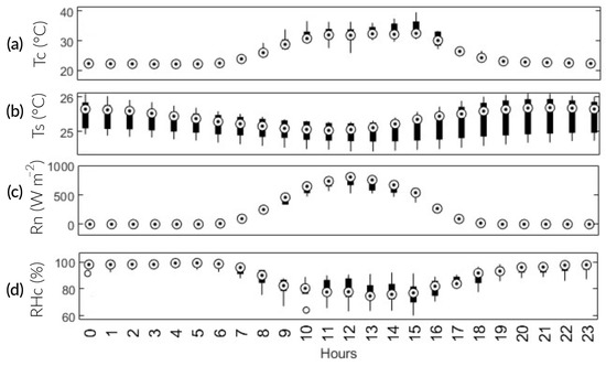
Figure 9.
Boxplot graphic: average diurnal variation in the main environmental factors. (a) Tc; (b) Ts; (c) Rn; and (d) RHc.
On the other hand, total NEE during the vegetative phase (−25.2 ) was 1.4 times lower than the minimum during the reproductive phase (−35 ). Similarly, the maximum diurnal NEE during the reproductive stage (−13 ) was 1.4 times higher than during the vegetative stage (−9.4 ). This is consistent with Yang et al. [21], who determined that the maximum absorption during the vegetative and maturation phase was approximately 1.5 times lower than in the reproductive phase. In the vegetative phase, CO2 assimilation is limited because the plant is in the growth stage (Figure 10a,b). In the reproductive stage, complete development is observed, leading to maximum absorption. In the maturation stage, senescent leaves fall and add organic matter to the soil. Additionally, the plots are drained in preparation for the harvest phase. These two processes gradually increase CO2 emissions until the crop is harvested (Figure 10c,d). This behavior is similar to the results of Chen et al. [30].
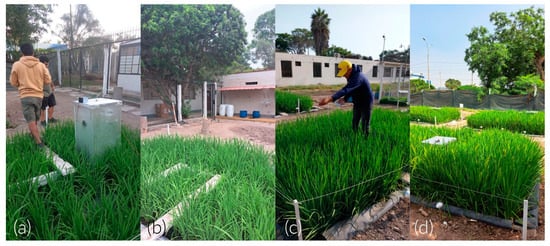
Figure 10.
Rice field growth in different stages of the cycle. (a–d) Tillering (82 and 89 DPS), spindle stage (111 DPS), and flowering (126 DPS).
4.2. NEE, Reco, and Their Interactions with Environmental Variables
The results for Reco showed a strong positive correlation with Tc and Rn. It is worth noting that these variables are strongly and positively related (R2 = 0.84). According to previous studies, Tc is an important factor in CO2 emissions from agricultural ecosystems [30,31]; the same applies to Rn. As Rn and Tc intensify throughout the day, root and microbial activity emits CO2 into the atmosphere. The maximum Reco occurs at 12:00 p.m. Nevertheless, photosynthetic activity is higher than Reco. In comparison with Bao et al. [27], it was observed that Reco had a weak negative correlation with Ts, possibly influenced by soil texture, ecosystem type, and water regime. In contrast, the seasonal variation in NEE was negatively related to Tc and Rn. Rn plays a crucial role as the primary energy source for plant metabolism. Consequently, when there is an increase in available energy, plants will absorb more CO2 (Figure 9c). These findings line up with the research conducted by Liu et al. [31].
Regarding Tc, the results are consistent with those of Bhattacharyya et al. [29] and Morales [32]. They found an inverse relationship between temperature and CO2 assimilation after surpassing 34 °C. This is because the rubisco enzyme, which is essential in CO2 fixation, is susceptible to thermal stress. Thus, the temperature inside the chamber exceeded this threshold at 82 DPS between 10:00 a.m. and 3:00 p.m. This may be a factor in why NEE is at its maximum throughout the season. Additionally, between 2:00 p.m. and 6:00 p.m., there is a 3.9-fold increase in CO2 emissions (Figure 9a). There is a weak positive correlation between NEE and Ts. Ts, in turn, has a weak negative correlation with Tc. This partially agrees with Liu et al. [31], as they did find a significantly high effect between Tc and Ts.
4.3. Comparison with Previous Studies
Information about the environmental and field management conditions from other authors is summarized in Table 4, as they influence CO2 absorption (Chen et al. [30] and Li et al. [33]).
Table 4.
Main environmental characteristics of the studies involved.
The results (Figure 11, Table A1, Table A2, Table A3 and Table A4) indicate a lower capacity for CO2 absorption than Chatterjee et al. [11], Kumar et al. [12], and Neogi et al. [13]; possibly influenced by climatic conditions. The study was under the conditions of a hot desert (Bwh) climate because of the permanent presence of the South Pacific anticyclone in northern Chile. On the other hand, Chatterjee et al. [11] and Neogi et al. [13] carried out their studies at the ICAR—National Rice Research Institute (NRRI) in India; they recorded climatic conditions typical of the tropical savanna type (Aw). For their part, Kumar et al. [12] at the Indian Agricultural Research Institute (IARI) in Dehli, India, were under hot semiarid climate conditions (Bsh).
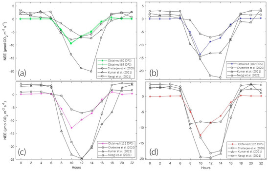
Figure 11.
Comparison of the diurnal variation in NEE in different stages of the rice phenological cycle. (a–d) Tillering, floral primordium, spindle stage, and flowering, respectively, cited in Chatterjee et al. [11], Kumar et al. [12] & Neogi et al. [13].
Regarding pp during the rice season, a total of 13.4 was recorded, despite the influence of the cyclone “Yaku,” which coincided with 111 and 126 DPS (Figure 2d). In comparison with Chatterjee et al. [11] and Neogi et al. [13], whose average annual pp was 1500 . 75 and 80% was happened between June and September. Kumar et al. [12], whose studies were carried out in Delhi, recorded 1198 during the kharif season for rice cultivation when most of the rains occur from July to September because of the southwest monsoon.
Regarding Tc, it ranged from 21.82 to 33.9 °C on average. On the other hand, Ts fluctuated between 24.95 and 25.51 °C on average. This study was carried out in the months of February to May during the summer season when the cold phase of the El Niño Southern Oscillation (ENSO) is also influential. Chatterjee et al. [11] recorded average annual maximum and minimum temperatures of 39.2 and 22.5 °C. Kumar et al. [12] recorded Ta and Ts values between 31.8 to 38.2 °C and 27.7 to 28.9 °C, respectively. Neogi et al. [13] recorded a progressive increase in temperature as the vegetative cycle of rice continued. From the vegetative stage to harvest, the average temperatures were 23.6 to 33.5 °C, respectively.
However, there were variations in the irrigation techniques used. This study had a maximum water depth of 5 during the entire study period. Chatterjee et al. [11] used a higher water regime in three units. Kumar et al. [12] irrigated their crops only when the moisture content fell below the saturation level. In turn, the irrigation regime of Neogi et al. [13] resulted in a sheet of 7–10 . According to Yang et al. [22], NEE is sensitive to field management strategies, with water management being one of the most important factors. In addition, soil CO2 emissions decrease when flooded with water, as this reduces the diffusivity of the upper layer of soil [34]. These anoxic conditions decrease soil biological activity, as mentioned by Bao et al. [27] and Liu et al. [31]. The result obtained from the Mann–Whitney U test shows that the NEE values did not present a significant difference between the analyzed studies (p > 0.05). Therefore, the CO2 analyzer generally performed optimally throughout the 24 h of monitoring and throughout the entire study period. However, more research is needed to consider it a reference method (Table 5).
Table 5.
Mann–Whitney U test for the values obtained compared with Chatterjee et al. [11], Kumar et al. [12], and Neogi et al. [13]. “**” indicates that there is no significant difference at the 0.05 level (p ≥ 0.05).
4.4. Portable Analyzer Performance
The MHZ19B sensor has a response time of less than 60 , so the analyzer was programmed with a response time of one minute to perform a better analysis. On the other hand, open-path analyzers such as LI—7500A and LI—7550 have selectable response times of 0.1, 0.05, and 0.0025 [35]. In addition, a regression analysis was performed between NEE fluxes calculated from data collected with the portable analyzer and NEE fluxes calculated using EC by Chatterjee et al. [11], Kumar et al. [12], and Neogi et al. [13]. The determination coefficients have values of 0.661, 0.7873, and 0.5943, respectively (Figure 12). These values can be improved if an additional calibration method is taken into consideration and by improving the Tc and RHc conditions. Furthermore, the sensitivity of the sensors is also an important factor to consider since the MHZ19B has a sensitivity of ±50 compared with LI—7500A, with ±0.11 [35].
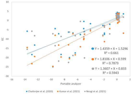
Figure 12.
Determination coefficients between NEE values (µmolCO2 m2 s−1) calculated with the portable analyzer and EC by Chatterjee et al. [11], Kumar et al. [12] & Neogi et al. [13]; respectively.
5. Conclusions
A static chamber with a portable CO2 analyzer was designed and implemented. It is an economical, simple, and effective alternative to traditional NEE calculation methods. It is a useful tool for making decisions about resource management in agricultural practice in Peru. Rice plots acted as a CO2 sink from 6:00 a.m. to 6:00 p.m. and as a CO2 source during the remaining period. The minimum NEE values at 82, 89, 102, 111, and 126 DPS were −9.51, −9.25, −13.63, −12.9, and −12.5 ; the maximum NEE values for the same dates were 0.68, 0.36, 0.32, 1, and 0.22 , respectively.
The total seasonal NEE values were −25.2 and −34.98 for the growth and reproductive stages, respectively. This represents a difference of 1.4 times between the mentioned stages. On the other hand, NEE was mainly influenced by Rn (R = −0.75), Tc (R = −0.69), and RHc (R = 0.66). NEE was negative throughout the rice growth period, demonstrating that the rice field acted as a net CO2 sink. The results did not show a significant difference compared with previous studies, indicating the optimal performance of the analyzer. Furthermore, differences in CO2 absorption can primarily be attributed to the type of crop, irrigation management, and climatic and soil conditions. These results are similar to previous studies obtained via chromatographic analysis and eddy covariance (EC), which suggests that the portable analyzer could be an alternative for CO2 monitoring.
Author Contributions
Conceptualization, L.R.-F.; methodology, M.B.-C. and I.E.-C.; validation, L.R.-F., L.F.d.P. and L.C.-V.; investigation, M.B.-C. and I.E.-C.; resources, L.R.-F., L.C.-V. and L.F.d.P.; data curation, L.R.-F., M.B.-C. and I.E.-C.; writing—original draft preparation, M.B.-C., I.E.-C. and L.R.-F.; writing—review and editing, L.R.-F., L.C.-V. and L.F.d.P.; supervision, L.R.-F., L.C.-V. and L.F.d.P.; project administration, L.R.-F. All authors have read and agreed to the published version of the manuscript.
Funding
This research was funded by National Scientific Research and Advanced Studies Program (PROCIENCIA) of PROCIENCIA-Peru, under the project “Implementation of the technological tool in the development of a precision system with remote sensors to optimize the use of water and reduce the emission of greenhouse gases in rice fields for the benefit of farmers in the Lambayeque region” (Contract: PE501078113-2022).
Institutional Review Board Statement
Not applicable.
Informed Consent Statement
Not applicable.
Data Availability Statement
The data presented in this study are available on request from the corresponding author.
Conflicts of Interest
The authors declare no conflicts of interest.
Appendix A
Table A1.
Comparison of the diurnal variation in NEE (µmolCO2 m2 s−1) in tillering.
Table A1.
Comparison of the diurnal variation in NEE (µmolCO2 m2 s−1) in tillering.
| Hour | PPFD Yang et al. [21] | DPS | References | |||
|---|---|---|---|---|---|---|
| 82 | 89 | Chatterjee et al. [11] | Kumar et al. [12] | Neogi et al. [13] | ||
| 0 | 10 | −0.061 ± 0.09 | 0.143 ± 0.25 | 3.439 | 1.84 | 2.459 |
| 2 | 10 | −0.069 ± 0.05 | 0.309 ± 0.29 | 1.186 | 1.58 | 2.295 |
| 4 | 10 | −0.041 ± 0.12 | 0.361 ± 0.39 | 0.593 | 2.91 | 2.459 |
| 6 | 10 | −0.064 ± 0.03 | 0.171 ± 0.21 | 0.356 | 0.53 | 2.787 |
| 8 | 200 | −4.148 ± 0.17 | −3.860 ± 0.54 | −1.660 | −5.55 | −4.754 |
| 10 | 600 | −9.511 ± 0.08 | −9.245 ± 0.54 | −4.387 | −7.93 | −13.607 |
| 12 | 400 | −6.555 ± 0.53 | −6.777 ± 0.91 | −6.759 | −7.14 | −18.852 |
| 14 | 300 | −4.710 ± 0.9 | −5.141 ± 0.63 | −5.929 | −7.40 | −20.164 |
| 16 | 100 | −0.928 ± 0.24 | −1.233 ± 0.77 | −2.016 | −4.36 | −7.213 |
| 18 | 10 | 0.686 ± 0.89 | - | 1.660 | −0.66 | 1.967 |
| 20 | 10 | 0.015 ± 0.18 | 0.280 ± 0.28 | 2.253 | 0.40 | 2.459 |
| 22 | 10 | −0.014 ± 0.04 | 0.247 ± 0.21 | 0.711 | 2.51 | 2.623 |
Table A2.
Comparison of the diurnal variation in NEE (µmolCO2 m2 s−1) in floral primordium.
Table A2.
Comparison of the diurnal variation in NEE (µmolCO2 m2 s−1) in floral primordium.
| Hour | PPFD Yang et al. [21] | DPS | References | ||
|---|---|---|---|---|---|
| 102 | Chatterjee et al. [11] | Kumar et al. [12] | Neogi et al. [13] | ||
| 0 | 10 | −0.034 ± 0.17 | 0.891 | 2.03 | 2.956 |
| 2 | 10 | −0.041 ± 0.05 | 1.040 | 1.50 | 3.103 |
| 4 | 10 | −0.036 ± 0.04 | 1.040 | 1.76 | 2.808 |
| 6 | 10 | 0.318 ± 0.3 | 0.149 | 1.24 | 2.956 |
| 8 | 200 | −4.997 ± 0.59 | −0.446 | −9.68 | −6.059 |
| 10 | 600 | −13.626 ± 0.54 | −5.792 | −14.55 | −15.517 |
| 12 | 400 | −8.829 ± 1.29 | −7.129 | −13.23 | −21.872 |
| 14 | 300 | −7.336 ± 0.48 | −6.238 | −13.10 | −22.611 |
| 16 | 100 | −2.123 ± 0.73 | −2.673 | −8.23 | −7.833 |
| 18 | 10 | 0.171 ± 0.21 | 1.782 | −1.00 | 2.069 |
| 20 | 10 | 0.110 ± 0.09 | 1.485 | −1.39 | 3.103 |
| 22 | 10 | 0.282 ± 0.24 | 1.634 | 3.60 | 3.103 |
Table A3.
Comparison of the diurnal variation in NEE (µmolCO2 m2 s−1) in spindle state.
Table A3.
Comparison of the diurnal variation in NEE (µmolCO2 m2 s−1) in spindle state.
| Hour | PPFD Yang et al. [21] | DPS | References | ||
|---|---|---|---|---|---|
| 111 | Chatterjee et al. [11] | Kumar et al. [12] | Neogi et al. [13] | ||
| 0 | 10 | 0.081 ± 0.19 | 3.939 | 3.15 | 0.891 |
| 2 | 10 | 0.194 ± 0.25 | 3.788 | 3.28 | 1.040 |
| 4 | 10 | 0.313 ± 0.47 | 3.788 | 3.41 | 1.040 |
| 6 | 10 | 0.290 ± 0.47 | 2.727 | 3.41 | 0.149 |
| 8 | 200 | −5.550 ± 0.36 | −7.576 | −14.14 | −0.446 |
| 10 | 600 | −12.901 ± 1.52 | −18.333 | −23.23 | −5.792 |
| 12 | 400 | −9.720 ± 0.32 | −25.000 | −24.75 | −7.129 |
| 14 | 300 | −7.202 ± 0.36 | −20.000 | −20.58 | −6.238 |
| 16 | 100 | −1.881 ± 0.69 | −7.424 | −11.36 | −2.673 |
| 18 | 10 | 1.003 ± 0.6 | 3.636 | −6.82 | 1.782 |
| 20 | 10 | 0.069 ± 0.21 | 4.394 | 2.65 | 1.485 |
| 22 | 10 | 0.321 ± 0.52 | 4.091 | 3.79 | 1.634 |
Table A4.
Comparison of the diurnal variation in NEE (µmolCO2 m2 s−1) in bloom.
Table A4.
Comparison of the diurnal variation in NEE (µmolCO2 m2 s−1) in bloom.
| Hour | PPFD Yang et al. [21] | DPS | References | ||
|---|---|---|---|---|---|
| 126 | Chatterjee et al. [11] | Kumar et al. [12] | Neogi et al. [13] | ||
| 0 | 10 | −0.084 ± 0.15 | 3.750 | 2.82 | 2.513 |
| 2 | 10 | −0.065 ± 0.19 | 3.750 | 2.69 | 2.932 |
| 4 | 10 | 0.059 ± 0.4 | 3.913 | 3.19 | 2.513 |
| 6 | 10 | 0.097 ± 0.5 | 3.098 | 2.44 | 1.675 |
| 8 | 200 | −5.021 ± 0.28 | −4.402 | −10.26 | −8.796 |
| 10 | 600 | −12.489 ± 1.12 | −13.207 | −19.43 | −8.168 |
| 12 | 400 | −8.468 ± 0.35 | −18.261 | −19.69 | −8.586 |
| 14 | 300 | −6.330 ± 0.28 | −17.446 | −18.43 | −8.168 |
| 16 | 100 | −1.899 ± 0.8 | −6.848 | −2.84 | −3.560 |
| 18 | 10 | 0.218 ± 0.42 | 1.793 | 3.44 | 1.885 |
| 20 | 10 | 0.074 ± 0.28 | 3.750 | 3.82 | 2.304 |
| 22 | 10 | 0.069 ± 0.3 | 3.587 | 1.06 | 2.094 |
References
- Change, N.G.C. Carbon Dioxide Concentration|NASA Global Climate Change. Available online: https://climate.nasa.gov/vital-signs/carbon-dioxide (accessed on 29 December 2023).
- Zhang, Y.; Liu, H.; Qi, J.; Feng, P.; Zhang, X.; Liu, D.L.; Marek, G.W.; Srinivasan, R.; Chen, Y. Assessing Impacts of Global Climate Change on Water and Food Security in the Black Soil Region of Northeast China Using an Improved SWAT-CO2 Model. Sci. Total Environ. 2023, 857, 159482. [Google Scholar] [CrossRef] [PubMed]
- Oo, A.Z.; Yamamoto, A.; Ono, K.; Umamageswari, C.; Mano, M.; Vanitha, K.; Elayakumar, P.; Matsuura, S.; Bama, K.S.; Raju, M.; et al. Ecosystem Carbon Dioxide Exchange and Water Use Efficiency in a Triple-Cropping Rice Paddy in Southern India: A Two-Year Field Observation. Sci. Total Environ. 2023, 854, 158541. [Google Scholar] [CrossRef] [PubMed]
- Kumar, A.; Nayak, A.K.; Das, B.S.; Panigrahi, N.; Dasgupta, P.; Mohanty, S.; Kumar, U.; Panneerselvam, P.; Pathak, H. Effects of Water Deficit Stress on Agronomic and Physiological Responses of Rice and Greenhouse Gas Emission from Rice Soil under Elevated Atmospheric CO2. Sci. Total Environ. 2019, 650, 2032–2050. [Google Scholar] [CrossRef] [PubMed]
- Gupta, K.; Kumar, R.; Baruah, K.K.; Hazarika, S.; Karmakar, S.; Bordoloi, N. Greenhouse Gas Emission from Rice Fields: A Review from Indian Context. Environ. Sci. Pollut. Res. 2021, 28, 30551–30572. [Google Scholar] [CrossRef]
- FAOSTAT. Available online: https://www.fao.org/faostat/es/#data/QCL (accessed on 29 December 2023).
- Gao, H.; Liu, Q.; Yan, C.; Wu, Q.; Gong, D.; He, W.; Liu, H.; Wang, J.; Mei, X. Mitigation of Greenhouse Gas Emissions and Improved Yield by Plastic Mulching in Rice Production. Sci. Total Environ. 2023, 880, 162984. [Google Scholar] [CrossRef]
- Liao, B.; Cai, T.; Wu, X.; Luo, Y.; Liao, P.; Zhang, B.; Zhang, Y.; Wei, G.; Hu, R.; Luo, Y.; et al. A Combination of Organic Fertilizers Partially Substitution with Alternate Wet and Dry Irrigation Could Further Reduce Greenhouse Gases Emission in Rice Field. J. Environ. Manag. 2023, 344, 118372. [Google Scholar] [CrossRef]
- Gangopadhyay, S.; Chowdhuri, I.; Das, N.; Pal, S.C.; Mandal, S. The Effects of No-Tillage and Conventional Tillage on Greenhouse Gas Emissions from Paddy Fields with Various Rice Varieties. Soil Tillage Res. 2023, 232, 105772. [Google Scholar] [CrossRef]
- Yang, S.; Sun, X.; Ding, J.; Jiang, Z.; Liu, X.; Xu, J. Effect of Biochar Addition on CO2 Exchange in Paddy Fields under Water-Saving Irrigation in Southeast China. J. Environ. Manag. 2020, 271, 111029. [Google Scholar] [CrossRef]
- Chatterjee, S.; Swain, C.K.; Nayak, A.K.; Chatterjee, D.; Bhattacharyya, P.; Mahapatra, S.S.; Debnath, M.; Tripathi, R.; Guru, P.K.; Dhal, B. Partitioning of Eddy Covariance-Measured Net Ecosystem Exchange of CO2 in Tropical Lowland Paddy. Paddy Water Environ. 2020, 18, 623–636. [Google Scholar] [CrossRef]
- Kumar, A.; Bhatia, A.; Sehgal, V.K.; Tomer, R.; Jain, N.; Pathak, H. Net Ecosystem Exchange of Carbon Dioxide in Rice-Spring Wheat System of Northwestern Indo-Gangetic Plains. Land 2021, 10, 701. [Google Scholar] [CrossRef]
- Neogi, S.; Bhattacharyya, P.; Nayak, A.K. Characterization of Carbon Dioxide Fluxes in Tropical Lowland Flooded Rice Ecology. Paddy Water Environ. 2021, 19, 539–552. [Google Scholar] [CrossRef]
- Klosterhalfen, A.; Chi, J.; Kljun, N.; Lindroth, A.; Laudon, H.; Nilsson, M.B.; Peichl, M. Two-Level Eddy Covariance Measurements Reduce Bias in Land-Atmosphere Exchange Estimates over a Heterogeneous Boreal Forest Landscape. Agric. For. Meteorol. 2023, 339, 109523. [Google Scholar] [CrossRef]
- Zhao, Y.; Wu, J.; Guo, C.; Wu, H.; Wang, J.; Zhang, Q.; Xiao, Y.; Qiu, R. Comparing the Eddy Covariance and Gradient Methods for Measuring Water and Heat Fluxes in Paddy Fields. Agric. Water Manag. 2023, 284, 108340. [Google Scholar] [CrossRef]
- Gao, D.; Yao, J.; Yu, S.; Ma, Y.; Li, L.; Gao, Z. Eddy Covariance CO2 Flux Gap Filling for Long Data Gaps: A Novel Framework Based on Machine Learning and Time Series Decomposition. Remote Sens. 2023, 15, 2695. [Google Scholar] [CrossRef]
- Li, J.; Xue, Z.; Li, Y.; Bo, G.; Shen, F.; Gao, X.; Zhang, J.; Tan, T. Real-Time Measurement of Atmospheric CO2, CH4 and N2O above Rice Fields Based on Laser Heterodyne Radiometers (LHR). Agronomy 2023, 13, 373. [Google Scholar] [CrossRef]
- Low-Cost IoT-Enabled Embedded System for Measurement of Environmental Pollutants—ProQuest. Available online: https://www.proquest.com/openview/98d3b4da3c59b80ae4541e3b6eb9ea60/1?pq-origsite=gscholar&cbl=2030013 (accessed on 29 December 2023).
- Rajasekar, P.; Selvi, J.A.V. Sensing and Analysis of Greenhouse Gas Emissions from Rice Fields to the Near Field Atmosphere. Sensors 2022, 22, 4141. [Google Scholar] [CrossRef] [PubMed]
- Coulby, G.; Clear, A.K.; Jones, O.; Godfrey, A. Low-Cost, Multimodal Environmental Monitoring Based on the Internet of Things. Build. Environ. 2021, 203, 108014. [Google Scholar] [CrossRef]
- Yang, S.; Xu, J.; Liu, X.; Zhang, J.; Wang, Y. Variations of Carbon Dioxide Exchange in Paddy Field Ecosystem under Water-Saving Irrigation in Southeast China. Agric. Water Manag. 2016, 166, 42–52. [Google Scholar] [CrossRef]
- Yang, S.; Liu, X.; Liu, X.; Xu, J. Effect of Water Management on Soil Respiration and NEE of Paddy Fields in Southeast China. Paddy Water Environ. 2017, 15, 787–796. [Google Scholar] [CrossRef]
- Pilegaard, K.; Hummelshøj, P.; Jensen, N.O.; Chen, Z. Two Years of Continuous CO2 Eddy-Flux Measurements over a Danish Beech Forest. Agric. For. Meteorol. 2001, 107, 29–41. [Google Scholar] [CrossRef]
- Bhattacharyya, P.; Neogi, S.; Roy, K.S.; Dash, P.K.; Nayak, A.K.; Mohapatra, T. Tropical Low Land Rice Ecosystem Is a Net Carbon Sink. Agric. Ecosyst. Environ. 2014, 189, 127–135. [Google Scholar] [CrossRef]
- McMillan, A.M.S.; Goulden, M.L.; Tyler, S.C. Stoichiometry of CH4 and CO2 Flux in a California Rice Paddy. J. Geophys. Res. Biogeosci. 2007, 112, G01008. [Google Scholar] [CrossRef]
- Carbon Dioxide Fluxes over Grassland Ecosystems in the Middle Tianshan Region of China with Eddy Covariance Method. Available online: https://www.researchsquare.com (accessed on 29 December 2023).
- Bao, Y.; Liu, T.; Duan, L.; Tong, X.; Zhang, Y.; Wang, G.; Singh, V.P. Variations and Controlling Factors of Carbon Dioxide and Methane Fluxes in a Meadow-Rice Ecosystem in a Semi-Arid Region. CATENA 2022, 215, 106317. [Google Scholar] [CrossRef]
- Chatterjee, D.; Swain, C.K.; Chatterjee, S.; Bhattacharyya, P.; Tripathi, R.; Lal, B.; Gautam, P.; Shahid, M.; Dash, P.K.; Dhal, B.; et al. Is the Energy Balance in a Tropical Lowland Rice Paddy Perfectly Closed? Atmósfera 2021, 34, 59–78. [Google Scholar] [CrossRef]
- Net Ecosystem CO2 Exchange and Carbon Cycling in Tropical Lowland Flooded Rice Ecosystem|Nutrient Cycling in Agroecosystems. Available online: https://link.springer.com/article/10.1007/s10705-013-9553-1 (accessed on 29 December 2023).
- Chen, C.; Li, D.; Gao, Z.; Tang, J.; Guo, X.; Wang, L.; Wan, B. Seasonal and Interannual Variations of Carbon Exchange over a Rice-Wheat Rotation System on the North China Plain. Adv. Atmos. Sci. 2015, 32, 1365–1380. [Google Scholar] [CrossRef]
- Liu, C.; Wu, Z.; Hu, Z.; Yin, N.; Islam, A.R.M.T.; Wei, Z. Characteristics and Influencing Factors of Carbon Fluxes in Winter Wheat Fields under Elevated CO2 Concentration. Environ. Pollut. 2022, 307, 119480. [Google Scholar] [CrossRef]
- Morales, D. Efecto de altas temperaturas en algunas variables del crecimiento y el intercambio gaseoso en plantas de tomate (Lycopersicon esculentum Mill. CV. AMALIA). Cultiv. Trop. 2006, 27, 45–48. [Google Scholar]
- Li, C.; Li, Z.; Zhang, F.; Lu, Y.; Duan, C.; Xu, Y. Seasonal Dynamics of Carbon Dioxide and Water Fluxes in a Rice-Wheat Rotation System in the Yangtze-Huaihe Region of China. Agric. Water Manag. 2023, 275, 107992. [Google Scholar] [CrossRef]
- Saito, M.; Miyata, A.; Nagai, H.; Yamada, T. Seasonal Variation of Carbon Dioxide Exchange in Rice Paddy Field in Japan. Agric. For. Meteorol. 2005, 135, 93–109. [Google Scholar] [CrossRef]
- LI-7500|Support. Available online: https://www.licor.com/env/support/LI-7500/home.html (accessed on 2 January 2024).
Disclaimer/Publisher’s Note: The statements, opinions and data contained in all publications are solely those of the individual author(s) and contributor(s) and not of MDPI and/or the editor(s). MDPI and/or the editor(s) disclaim responsibility for any injury to people or property resulting from any ideas, methods, instructions or products referred to in the content. |
© 2024 by the authors. Licensee MDPI, Basel, Switzerland. This article is an open access article distributed under the terms and conditions of the Creative Commons Attribution (CC BY) license (https://creativecommons.org/licenses/by/4.0/).