

Validation of Machine Learning-Aided and Power Line Communication-Based Cable Monitoring Using Measurement Data


Abstract
1. Introduction
1.1. Background and Motivation
1.2. Challenges and Contributions
1.3. Related Work
1.4. Organization of the Paper
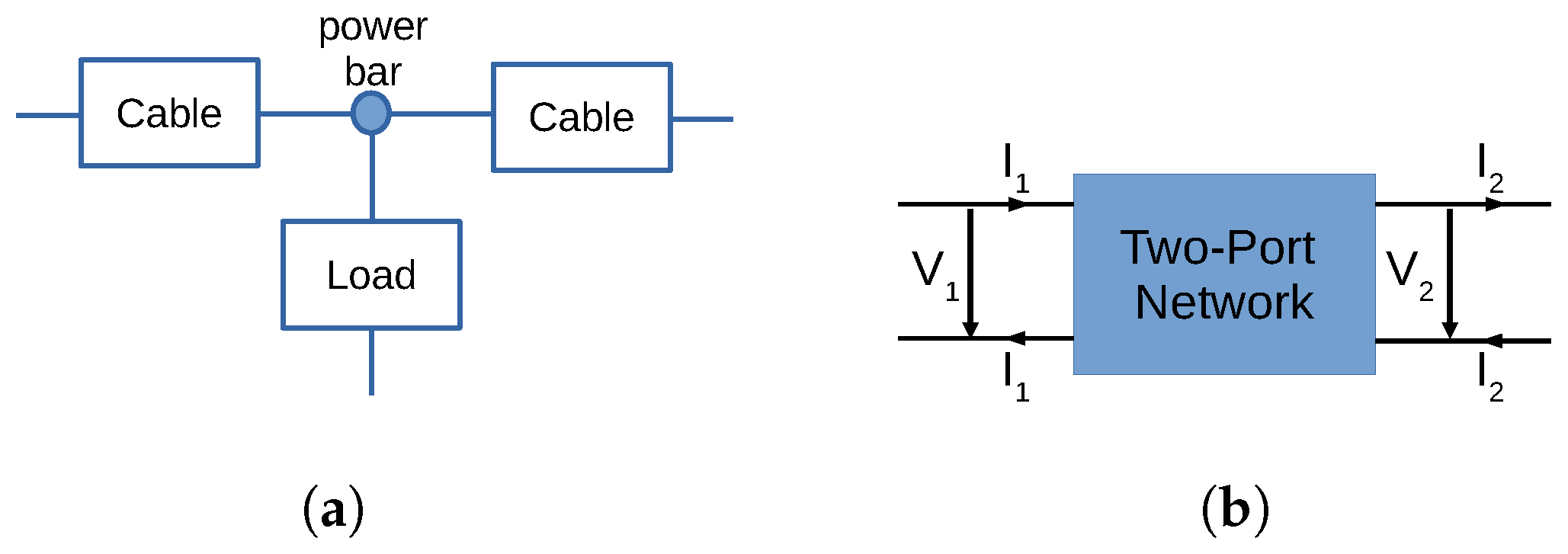
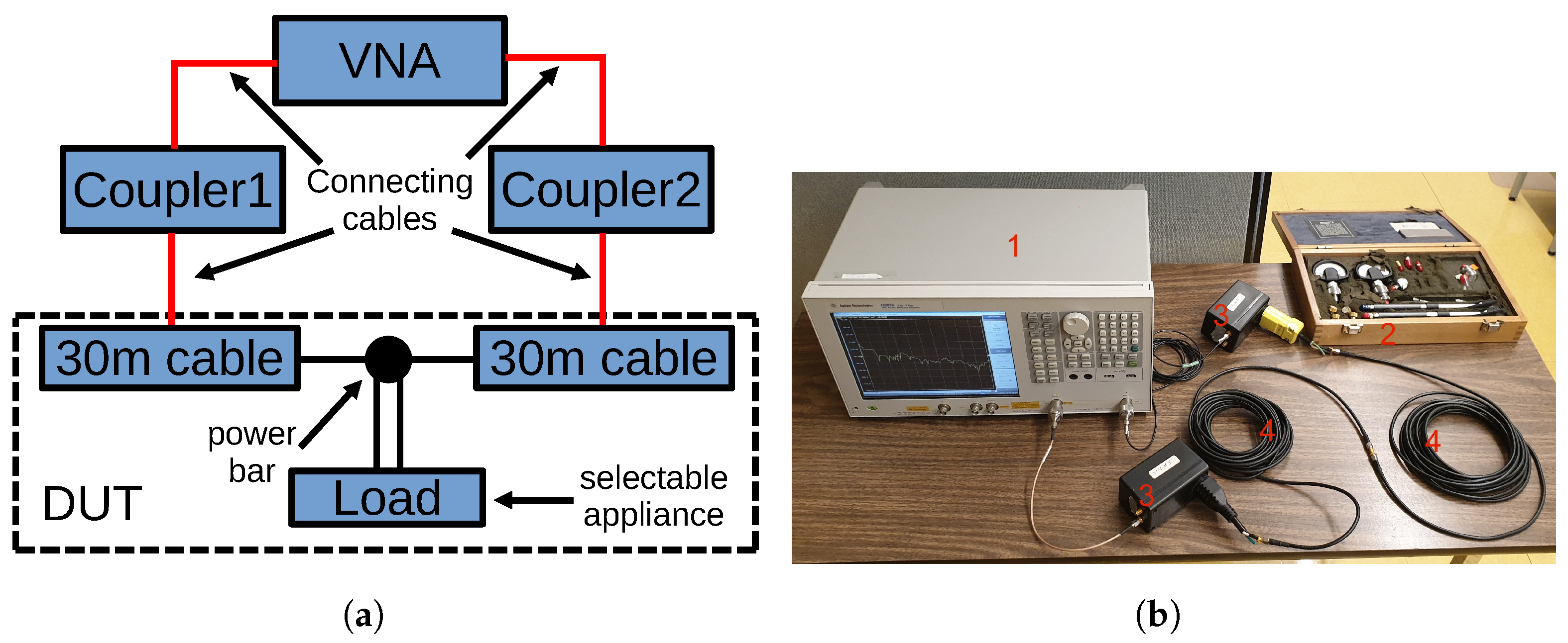
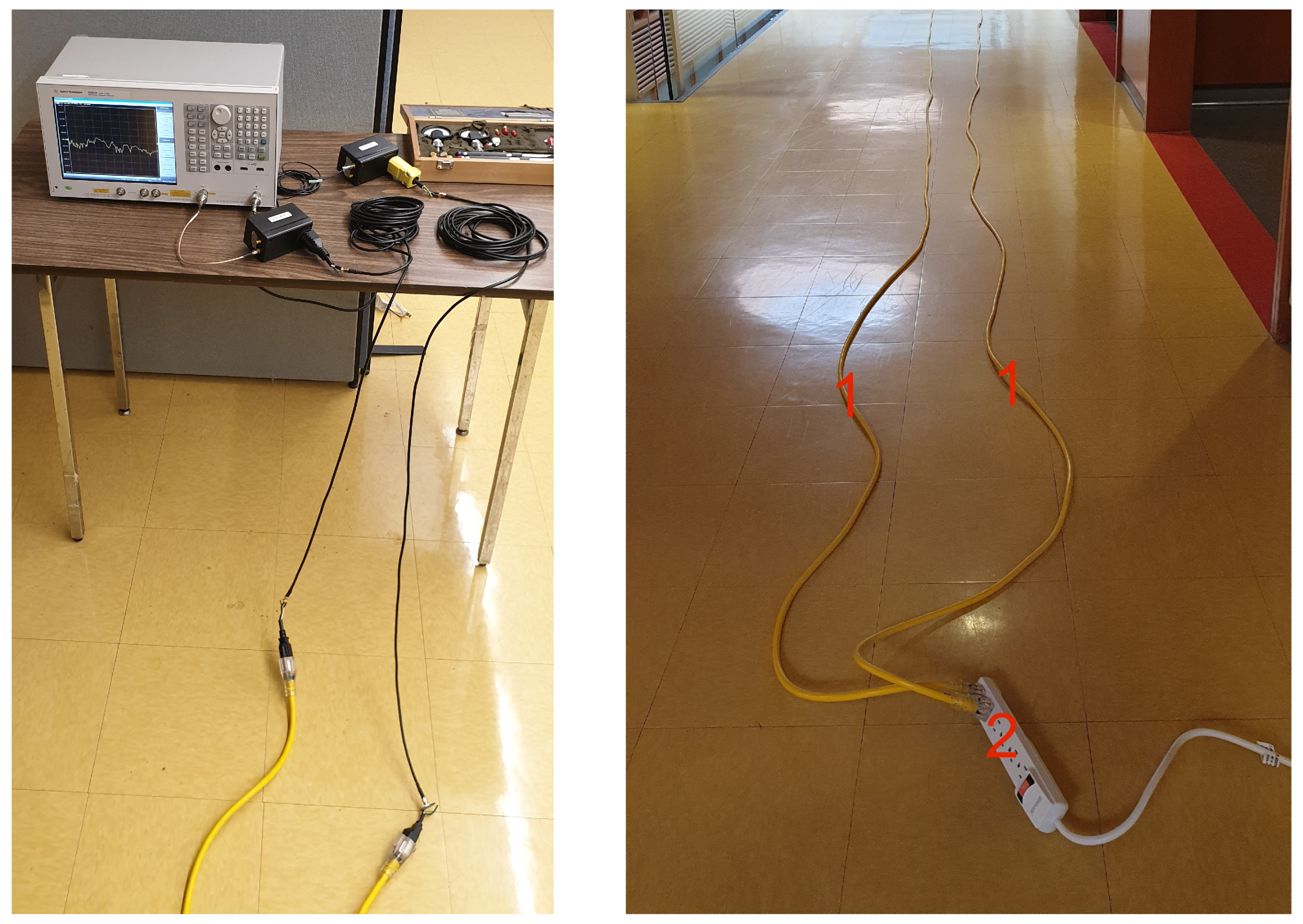
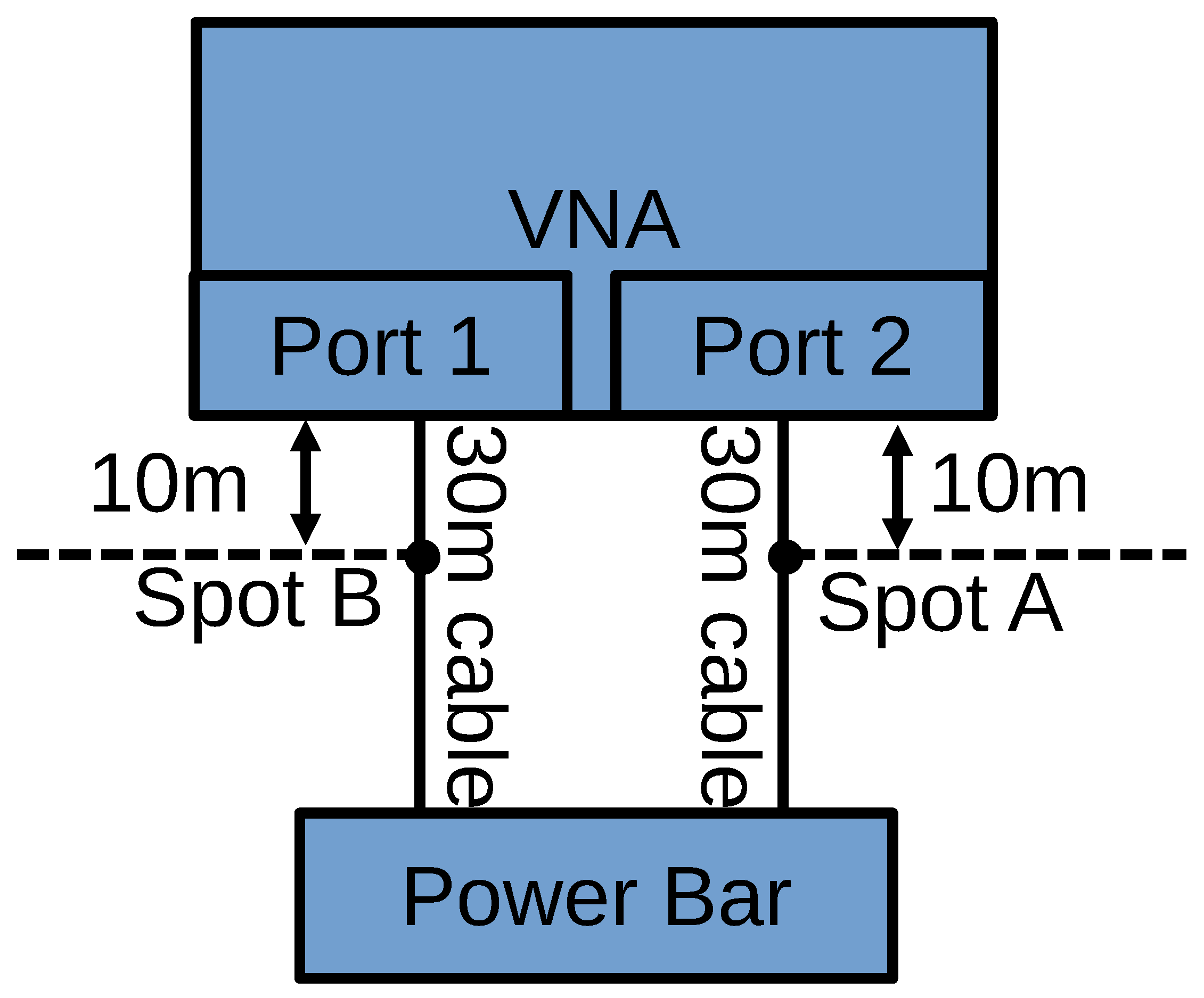
2. Experimental Setup
2.1. Two-Port Networks
2.2. Calibration
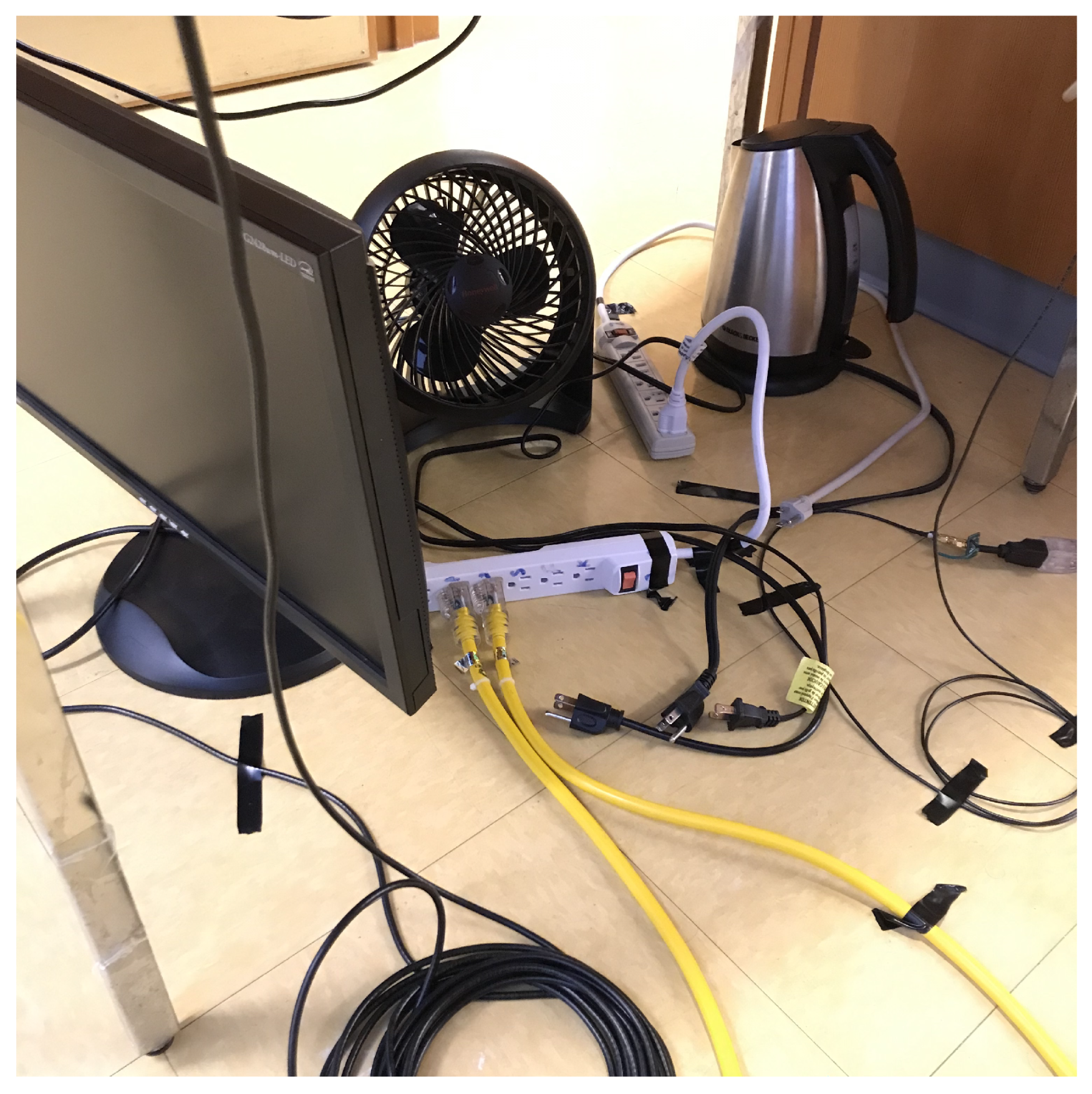
2.3. Measurements
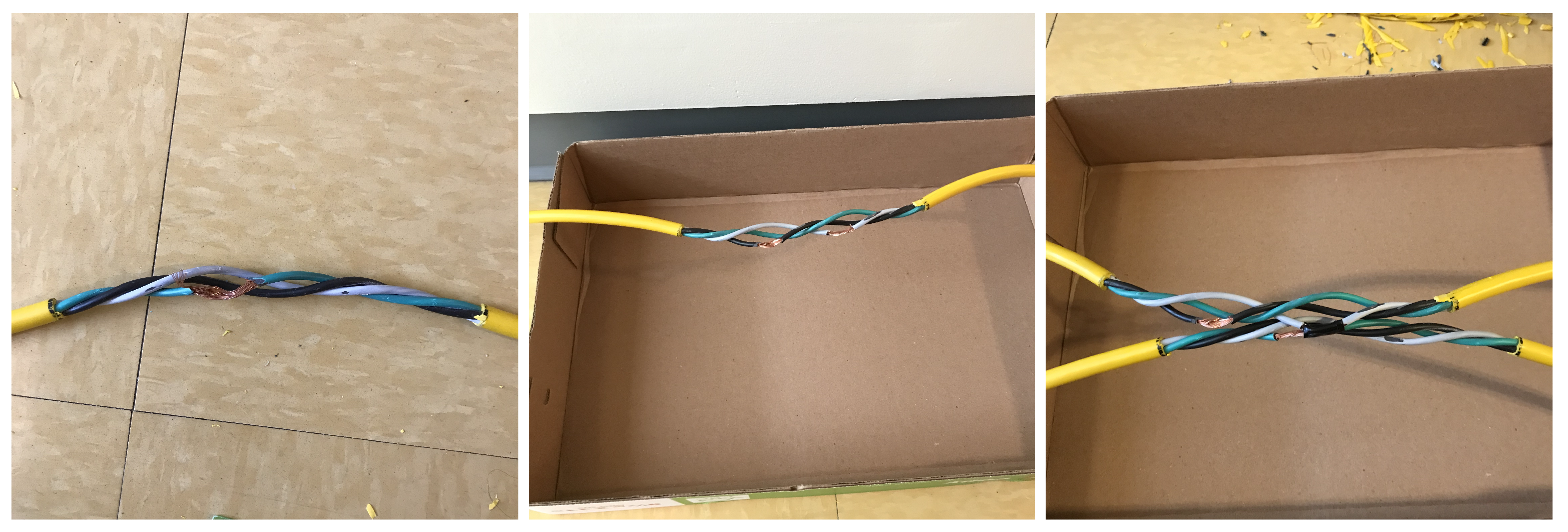
2.4. Manually Applied Degradations
3. PCA-Based Anomaly Detection
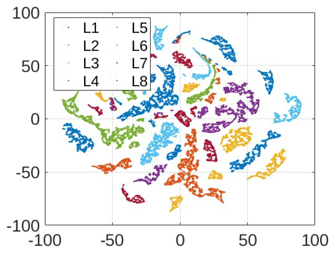
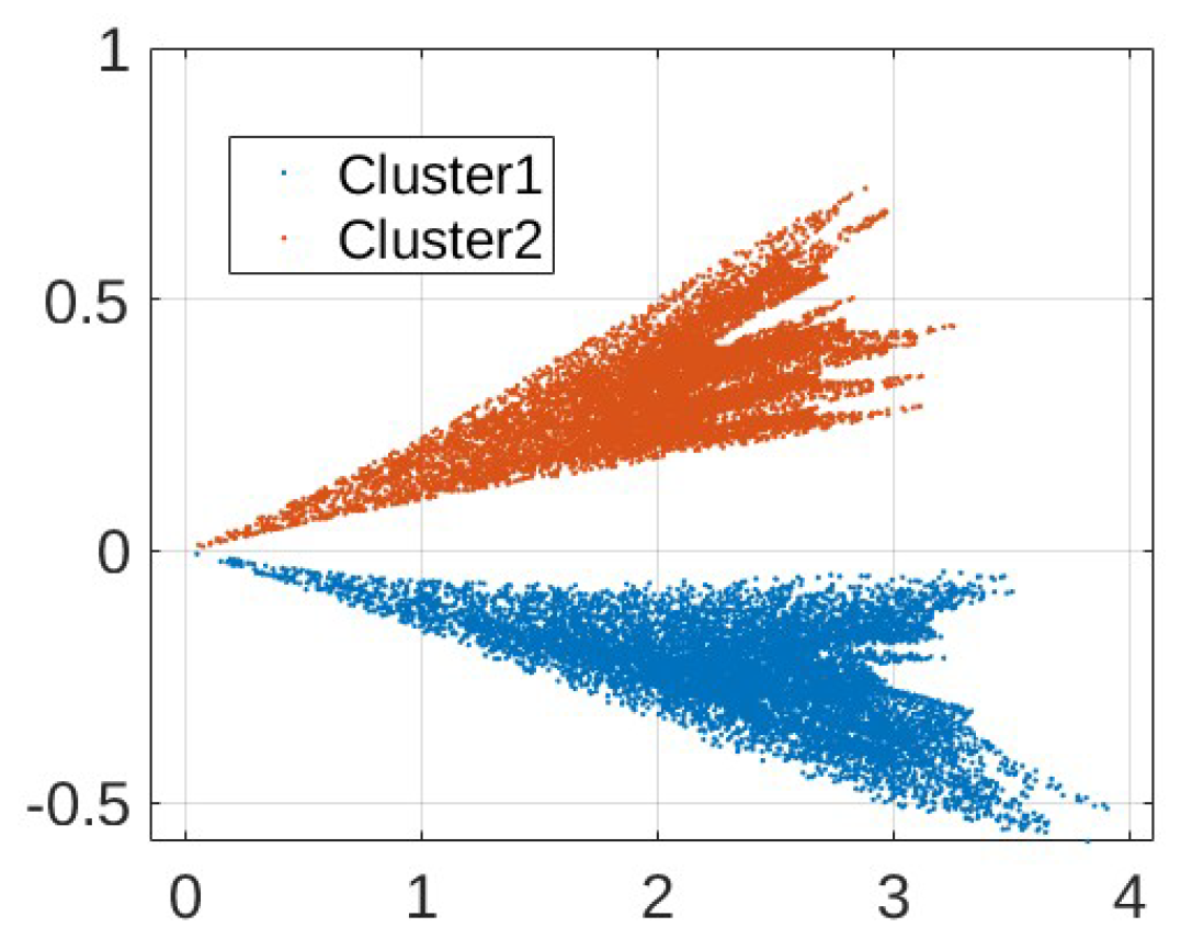
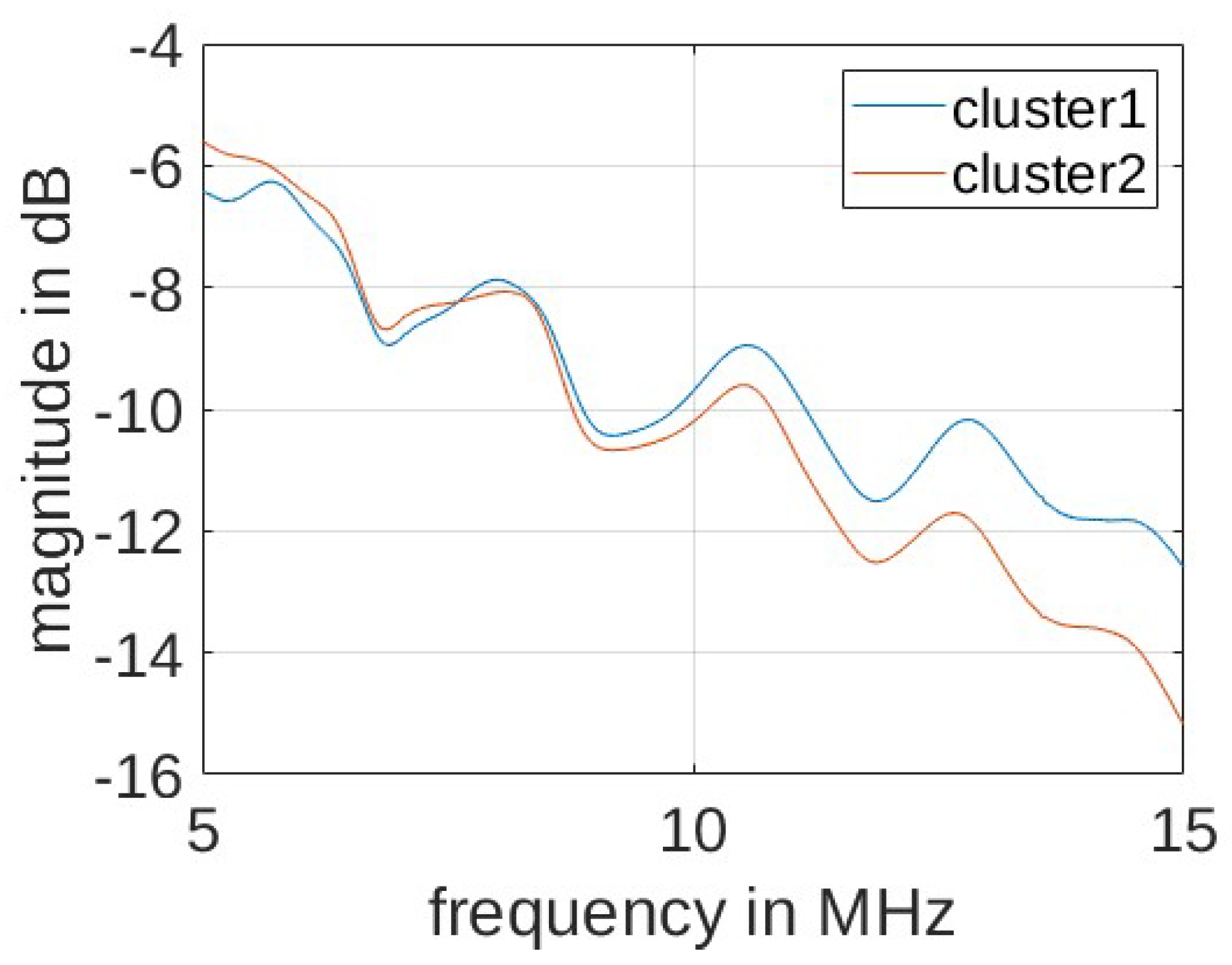
3.1. Clustering for Data Pre-Processing
3.2. PCA Background
3.3. PCA for Anomaly Detection
3.4. Implementation Details
4. Results
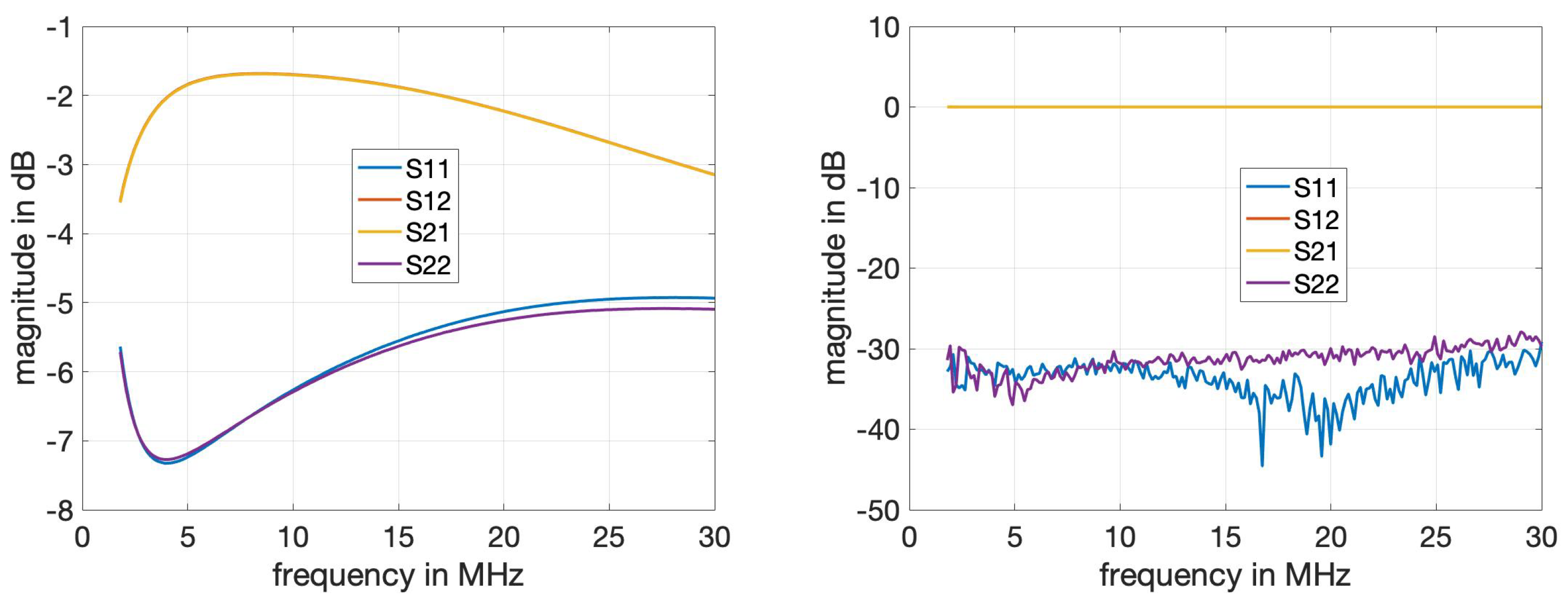
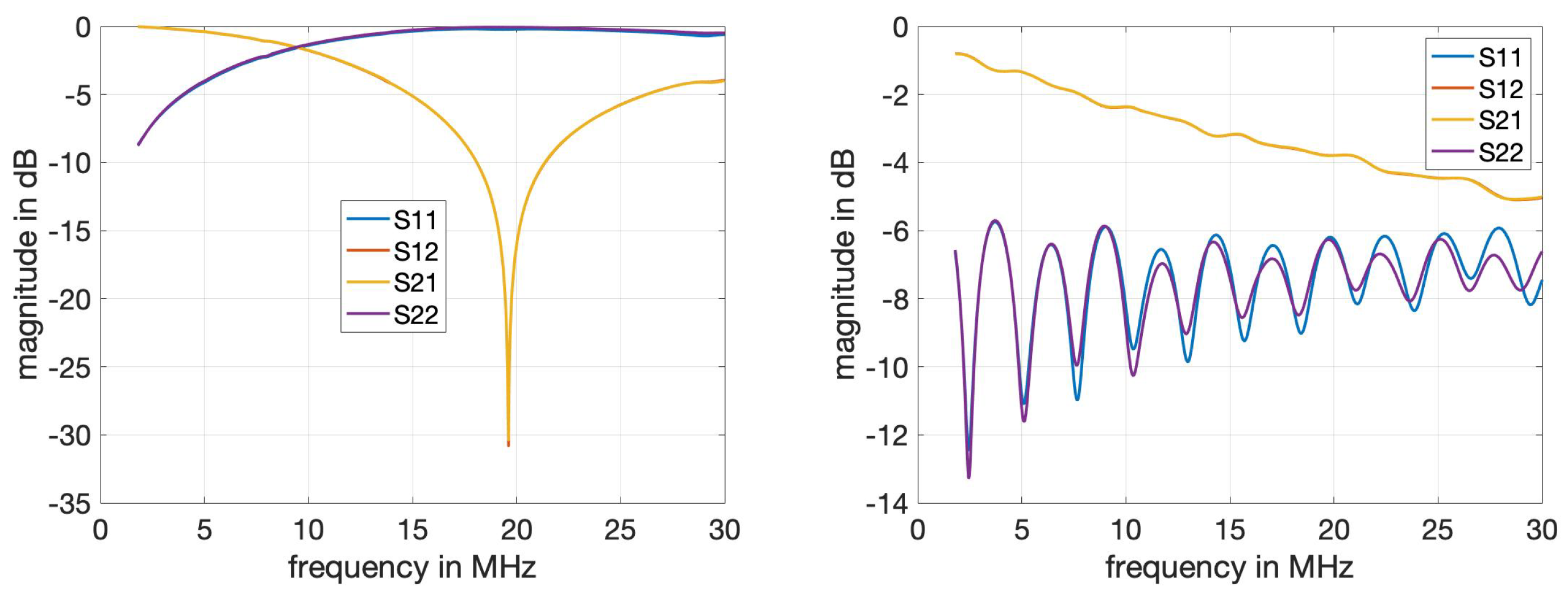
4.1. Calibration and Measurement of Components
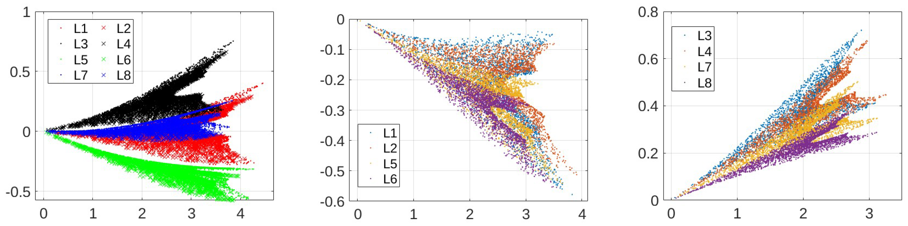
4.2. Data Generation and Pre-Processing
4.3. PCA Results
4.4. Discussion
5. Conclusions
Author Contributions
Funding
Institutional Review Board Statement
Informed Consent Statement
Data Availability Statement
Conflicts of Interest
References
- Farhangi, H. The path of the smart grid. IEEE Power Energy Mag. 2010, 8, 18–28. [Google Scholar] [CrossRef]
- Gill, P. Electrical Power Equipment Maintenance and Testing; CRC Press: Boca Raton, FL, USA, 2008. [Google Scholar]
- Galli, S.; Scaglione, A.; Wang, Z. For the Grid and Through the Grid: The Role of Power Line Communications in the Smart Grid. Proc. IEEE 2011, 99, 998–1027. [Google Scholar] [CrossRef]
- Huo, Y.; Prasad, G.; Atanackovic, L.; Lampe, L.; Leung, V.C.M. Grid Surveillance and Diagnostics using Power Line Communications. In Proceedings of the IEEE International Symposium on Power Line Communications and Its Applications (ISPLC), Manchester, UK, 8–11 April 2018; pp. 1–6. [Google Scholar]
- Lehmann, A.M.; Raab, K.; Gruber, F.; Fischer, E.; Müller, R.; Huber, J.B. A diagnostic method for power line networks by channel estimation of PLC devices. In Proceedings of the 2016 IEEE International Conference on Smart Grid Communications (SmartGridComm), Sydney, Australia, 6–9 November 2016; pp. 320–325. [Google Scholar] [CrossRef]
- Förstel, L.; Lampe, L. Grid diagnostics: Monitoring cable aging using power line transmission. In Proceedings of the 2017 IEEE International Symposium on Power Line Communications and Its Applications (ISPLC), Madrid, Spain, 3–5 April 2017; pp. 1–6. [Google Scholar] [CrossRef]
- Passerini, F.; Tonello, A.M. Smart grid monitoring using power line modems: Anomaly detection and localization. IEEE Trans. Smart Grid 2019, 10, 6178–6186. [Google Scholar] [CrossRef]
- Huo, Y.; Prasad, G.; Atanackovic, L.; Lampe, L.; Leung, V.C.M. Cable Diagnostics With Power Line Modems for Smart Grid Monitoring. IEEE Access 2019, 7, 60206–60220. [Google Scholar] [CrossRef]
- Milioudis, A.N.; Andreou, G.T.; Labridis, D.P. Detection and location of high impedance faults in multiconductor overhead distribution lines using power line communication devices. IEEE Trans. Smart Grid 2014, 6, 894–902. [Google Scholar] [CrossRef]
- Pittolo, A.; Tonello, A. A Synthetic Statistical MIMO PLC Channel Model Applied to an In-Home Scenario. IEEE Trans. Commun. 2017, 65, 2543–2553. [Google Scholar] [CrossRef]
- Gruber, F.; Lampe, L. On PLC channel emulation via transmission line theory. In Proceedings of the IEEE International Symposium on Power Line Communications and Its Applications (ISPLC), Austin, TX, USA, 29 March–1 April 2015; pp. 178–183. [Google Scholar] [CrossRef]
- Versolatto, F.; Tonello, A.M. An MTL Theory Approach for the Simulation of MIMO Power-Line Communication Channels. IEEE Trans. Power Deliv. 2011, 26, 1710–1717. [Google Scholar] [CrossRef]
- Huo, Y.; Prasad, G.; Lampe, L.; Leung, V.C.M.; Vijay, R.; Prabhakar, T. Measurement Aided Training of Machine Learning Techniques for Fault Detection Using PLC Signals. In Proceedings of the 2021 IEEE International Symposium on Power Line Communications and Its Applications (ISPLC), Aachen, Germany, 25–26 October 2021; pp. 78–83. [Google Scholar]
- Jiang, Y. Data-Driven Fault Location of Electric Power Distribution Systems With Distributed Generation. IEEE Trans. Smart Grid 2020, 11, 129–137. [Google Scholar] [CrossRef]
- Shi, X.; Qiu, R.; Ling, Z.; Yang, F.; Yang, H.; He, X. Spatio-Temporal Correlation Analysis of Online Monitoring Data for Anomaly Detection and Location in Distribution Networks. IEEE Trans. Smart Grid 2020, 11, 995–1006. [Google Scholar] [CrossRef]
- Shahsavari, A.; Farajollahi, M.; Stewart, E.; Cortez, E.; Mohsenian-Rad, H. Situational Awareness in Distribution Grid Using Micro-PMU Data: A Machine Learning Approach. IEEE Trans. Smart Grid 2019, 10, 6167–6177. [Google Scholar] [CrossRef]
- Seyedi, Y.; Karimi, H.; Grijalva, S. Irregularity Detection in Output Power of Distributed Energy Resources Using PMU Data Analytics in Smart Grids. IEEE Trans. Ind. Inform. 2018, 15, 2222–2232. [Google Scholar] [CrossRef]
- Shi, S.; Zhu, B.; Lei, A.; Dong, X. Fault Location for Radial Distribution Network via Topology and Reclosure-Generating Traveling Waves. IEEE Trans. Smart Grid 2019, 10, 6404–6413. [Google Scholar] [CrossRef]
- Sun, M.; Konstantelos, I.; Strbac, G. A Deep Learning-Based Feature Extraction Framework for System Security Assessment. IEEE Trans. Smart Grid 2019, 10, 5007–5020. [Google Scholar] [CrossRef]
- Zhao, Y.; Chen, J.; Poor, H.V. A Learning-to-Infer Method for Real-Time Power Grid Multi-Line Outage Identification. IEEE Trans. Smart Grid 2020, 11, 555–564. [Google Scholar] [CrossRef]
- Kiaei, I.; Lotfifard, S. Fault Section Identification in Smart Distribution Systems Using Multi-Source Data Based on Fuzzy Petri Nets. IEEE Trans. Smart Grid 2020, 11, 74–83. [Google Scholar] [CrossRef]
- Wang, X.; Gao, J.; Wei, X.; Song, G.; Wu, L.; Liu, J.; Zeng, Z.; Kheshti, M. High Impedance Fault Detection Method Based on Variational Mode Decomposition and Teager–Kaiser Energy Operators for Distribution Network. IEEE Trans. Smart Grid 2019, 10, 6041–6054. [Google Scholar] [CrossRef]
- Taylor, V.; Faulkner, M. Line monitoring and fault location using spread spectrum on power line carrier. IEE Proc.-Gener. Transm. Distrib. 1996, 143, 427–434. [Google Scholar] [CrossRef]
- Milioudis, A.N.; Andreou, G.T.; Labridis, D.P. Enhanced protection scheme for smart grids using power line communications techniques—Part II: Location of high impedance fault position. IEEE Trans. Smart Grid 2012, 3, 1631–1640. [Google Scholar] [CrossRef]
- Rao, R.; Akella, S.; Guley, G. Power line carrier (PLC) signal analysis of smart meters for outlier detection. In Proceedings of the IEEE International Conference on Smart Grid Communications (SmartGridComm), Brussels, Belgium, 17–20 October 2011; pp. 291–296. [Google Scholar]
- Alam, M.N.; Bhuiyan, R.H.; Dougal, R.A.; Ali, M. Design and application of surface wave sensors for nonintrusive power line fault detection. IEEE Sens. J. 2012, 13, 339–347. [Google Scholar] [CrossRef]
- Passerini, F.; Tonello, A.M. Full duplex power line communication modems for network sensing. In Proceedings of the 2017 IEEE International Conference on Smart Grid Communications (SmartGridComm), Dresden, Germany, 23–26 October 2017; pp. 1–5. [Google Scholar]
- Passerini, F.; Tonello, A.M. Analysis of High-Frequency Impedance Measurement Techniques for Power Line Network Sensing. IEEE Sens. J. 2017, 17, 7630–7640. [Google Scholar] [CrossRef]
- Prasad, G.; Huo, Y.; Lampe, L.; Mengi, A.; Leung, V.C.M. Fault Diagnostics with Legacy Power Line Modems. In Proceedings of the IEEE International Symposium on Power Line Communications and its Applications (ISPLC), Prague, Czech Republic, 3–5 April 2019; pp. 1–6. [Google Scholar]
- Lim, H.; Kwon, G.Y.; Shin, Y.J. Fault detection and localization of shielded cable via optimal detection of time–frequency-domain reflectometry. IEEE Trans. Instrum. Meas. 2021, 70, 1–10. [Google Scholar] [CrossRef]
- Robles, G.; Shafiq, M.; Martínez-Tarifa, J.M. Multiple partial discharge source localization in power cables through power spectral separation and time-domain reflectometry. IEEE Trans. Instrum. Meas. 2019, 68, 4703–4711. [Google Scholar] [CrossRef]
- Möhring, B.N.; Siart, U.; Eibert, T.F. Fast chirp frequency-modulated continuous-wave reflectometer for monitoring fast varying discontinuities on transmission lines. IEEE Trans. Instrum. Meas. 2021, 70, 1–11. [Google Scholar] [CrossRef]
- Huo, Y.; Prasad, G.; Lampe, L.; Leung, V.C.M. Smart-grid monitoring: Enhanced machine learning for cable diagnostics. In Proceedings of the IEEE International Symposium on Power Line Communications and its Applications (ISPLC), Prague, Czech Republic, 3–5 April 2019; pp. 1–6. [Google Scholar]
- Prasad, G.; Lampe, L. Full-duplex power line communications: Design and applications from multimedia to smart grid. IEEE Commun. Mag. 2019, 58, 106–112. [Google Scholar] [CrossRef]
- Milioudis, A.; Andreou, G.; Labridis, D. High impedance fault detection using power line communication techniques. In Proceedings of the 45th International Universities Power Engineering Conference UPEC2010, Cardiff, UK, 31 August–3 September 2010; pp. 1–6. [Google Scholar]
- Huo, Y.; Prasad, G.; Lampe, L.; Leung, V.C.M. Power Line Communication and Sensing Using Time Series Forecasting. Sensors 2022, 22, 5320. [Google Scholar] [CrossRef]
- Bondorf, M.; Koch, M.; Hopfer, N.; Zdrallek, M.; Balada, C.; Ahmed, S.; Agne, S.; Dengel, A.; Karl, F.; Dietzler, U.; et al. Broadband power line communication and big-data-analytics for supporting grid operation. In Proceedings of the ETG Congress 2021, Online, 18–19 March 2021; pp. 1–6. [Google Scholar]
- Frickey, D. Conversions between S, Z, Y, H, ABCD, and T parameters which are valid for complex source and load impedances. IEEE Trans. Microw. Theory Tech. 1994, 42, 205–211. [Google Scholar] [CrossRef]
- Natalino, C.; Udalcovs, A.; Wosinska, L.; Ozolins, O.; Furdek, M. Spectrum anomaly detection for optical network monitoring using deep unsupervised learning. IEEE Commun. Lett. 2021, 25, 1583–1586. [Google Scholar] [CrossRef]
- Adam, T.; Babič, F. Anomaly Detection on Distributed Ledger Using Unsupervised Machine Learning. In Proceedings of the IEEE International Conference on Omni-layer Intelligent Systems (COINS), Berlin, Germany, 23–25 July 2023; pp. 1–4. [Google Scholar]
- Zhang, L.; Lin, J.; Karim, R. Adaptive kernel density-based anomaly detection for nonlinear systems. Knowl.-Based Syst. 2018, 139, 50–63. [Google Scholar] [CrossRef]
- Abdi, H.; Williams, L.J. Principal component analysis. WIREs Comput. Stat. 2010, 2, 433–459. [Google Scholar] [CrossRef]
- Wang, W.; Guan, X.; Zhang, X. A novel intrusion detection method based on principle component analysis in computer security. In Proceedings of the International Symposium on Neural Networks; Springer: Berlin/Heidelberg, Germany, 2004; pp. 657–662. [Google Scholar]
- Huo, Y.; Prasad, G.; Lampe, L.; Leung, V.C.M. Advanced smart grid monitoring: Intelligent cable diagnostics using neural networks. In Proceedings of the 2020 IEEE International Symposium on Power Line Communications and its Applications (ISPLC), Malaga, Spain, 11–13 May 2020; pp. 1–6. [Google Scholar]


| Load Condition | Kettle | Fan | Monitor |
|---|---|---|---|
| L1 | - | - | - |
| L2 | ✓ | - | - |
| L3 | - | ✓ | - |
| L4 | ✓ | ✓ | - |
| L5 | - | - | ✓ |
| L6 | ✓ | - | ✓ |
| L7 | - | ✓ | ✓ |
| L8 | ✓ | ✓ | ✓ |
| (a) | ||||
| Threshold | ||||
| Stage 0 FA | ||||
| Stage 1 DA | 1 | 1 | 1 | |
| Stage 2 DA | 1 | 1 | 1 | |
| Stage 3 DA | 1 | 1 | 1 | |
| Stage 4 DA | 1 | 1 | 1 | |
| Stage 5 DA | 1 | 1 | 1 | |
| Stage 6 DA | 1 | 1 | 1 | |
| Stage 7 DA | 1 | 1 | 1 | |
| (b) | ||||
| Threshold | ||||
| non-energized | Stage 0 FA | |||
| Stage 1 DA | ||||
| Stage 2 DA | ||||
| Stage 3 DA | ||||
| Stage 4 DA | ||||
| Stage 5 DA | ||||
| Stage 6 DA | ||||
| Stage 7 DA | 1 | |||
| energized | Stage 0 FA | |||
| Stage 1 DA | ||||
| Stage 2 DA | ||||
| Stage 3 DA | ||||
| Stage 4 DA | ||||
| Stage 5 DA | ||||
| Stage 6 DA | ||||
| Stage 7 DA | 1 | |||
Disclaimer/Publisher’s Note: The statements, opinions and data contained in all publications are solely those of the individual author(s) and contributor(s) and not of MDPI and/or the editor(s). MDPI and/or the editor(s) disclaim responsibility for any injury to people or property resulting from any ideas, methods, instructions or products referred to in the content. |
© 2024 by the authors. Licensee MDPI, Basel, Switzerland. This article is an open access article distributed under the terms and conditions of the Creative Commons Attribution (CC BY) license (https://creativecommons.org/licenses/by/4.0/).
Share and Cite
Huo, Y.; Wang, K.; Lampe, L.; Leung, V.C.M. Validation of Machine Learning-Aided and Power Line Communication-Based Cable Monitoring Using Measurement Data. Sensors 2024, 24, 335. https://doi.org/10.3390/s24020335
Huo Y, Wang K, Lampe L, Leung VCM. Validation of Machine Learning-Aided and Power Line Communication-Based Cable Monitoring Using Measurement Data. Sensors. 2024; 24(2):335. https://doi.org/10.3390/s24020335
Chicago/Turabian StyleHuo, Yinjia, Kevin Wang, Lutz Lampe, and Victor C.M. Leung. 2024. "Validation of Machine Learning-Aided and Power Line Communication-Based Cable Monitoring Using Measurement Data" Sensors 24, no. 2: 335. https://doi.org/10.3390/s24020335
APA StyleHuo, Y., Wang, K., Lampe, L., & Leung, V. C. M. (2024). Validation of Machine Learning-Aided and Power Line Communication-Based Cable Monitoring Using Measurement Data. Sensors, 24(2), 335. https://doi.org/10.3390/s24020335