
Wearable Robot Design Optimization Using Closed-Form Human–Robot Dynamic Interaction Model

Abstract
1. Introduction
- (a)
- Defining assistive objectives of the robot in terms of unknown forces and torques in the human-robot system of equations of equilibrium to keep it statically determinate, allowing to solve it directly without optimization.
- (b)
- Using the technique developed by Shahabpoor and Pavic [16] to estimate the walking GRFs from the reference measured kinematic data, avoiding the need to measure walking GRFs.
- (1)
- Computational efficiency: the combination of a simplified link segment model and directly solving the system of equations for joint and interaction forces and torques without optimization makes the process highly computationally efficient. This, not only allows for effortless offline design optimization of the robot, but also allows the framework to be used online as part of the robot controller for real-time calculation of assistive torques.
- (2)
- Transparency: the clear mathematical formulation of the human–robot system allows for direct analysis of the relationship between the robot interventions and the consequent changes in human kinematics and kinetics.
- (3)
- Less prone to input errors due to the limited number of assumptions and uncertain inputs used.
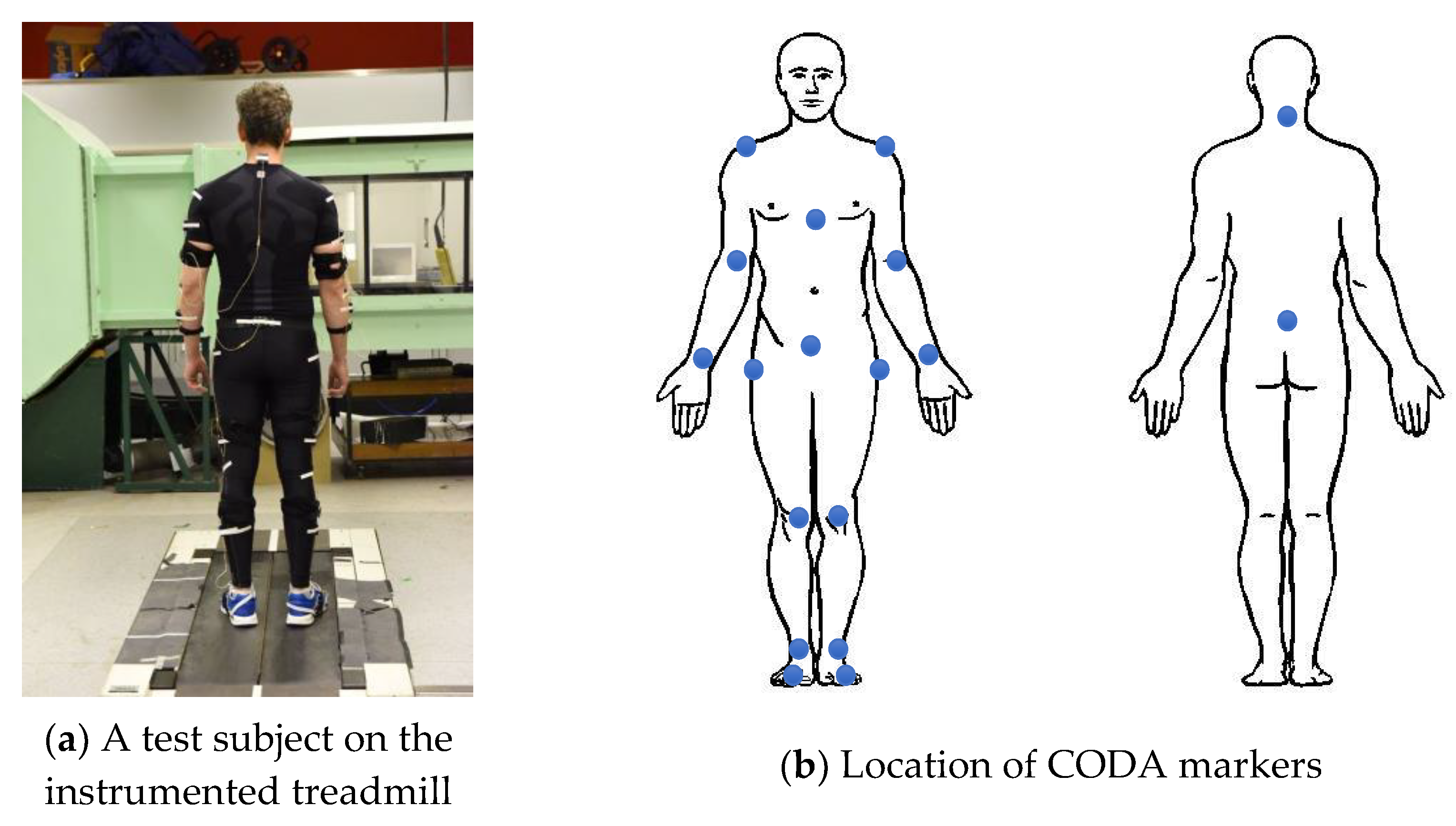
2. Experimental Measurements
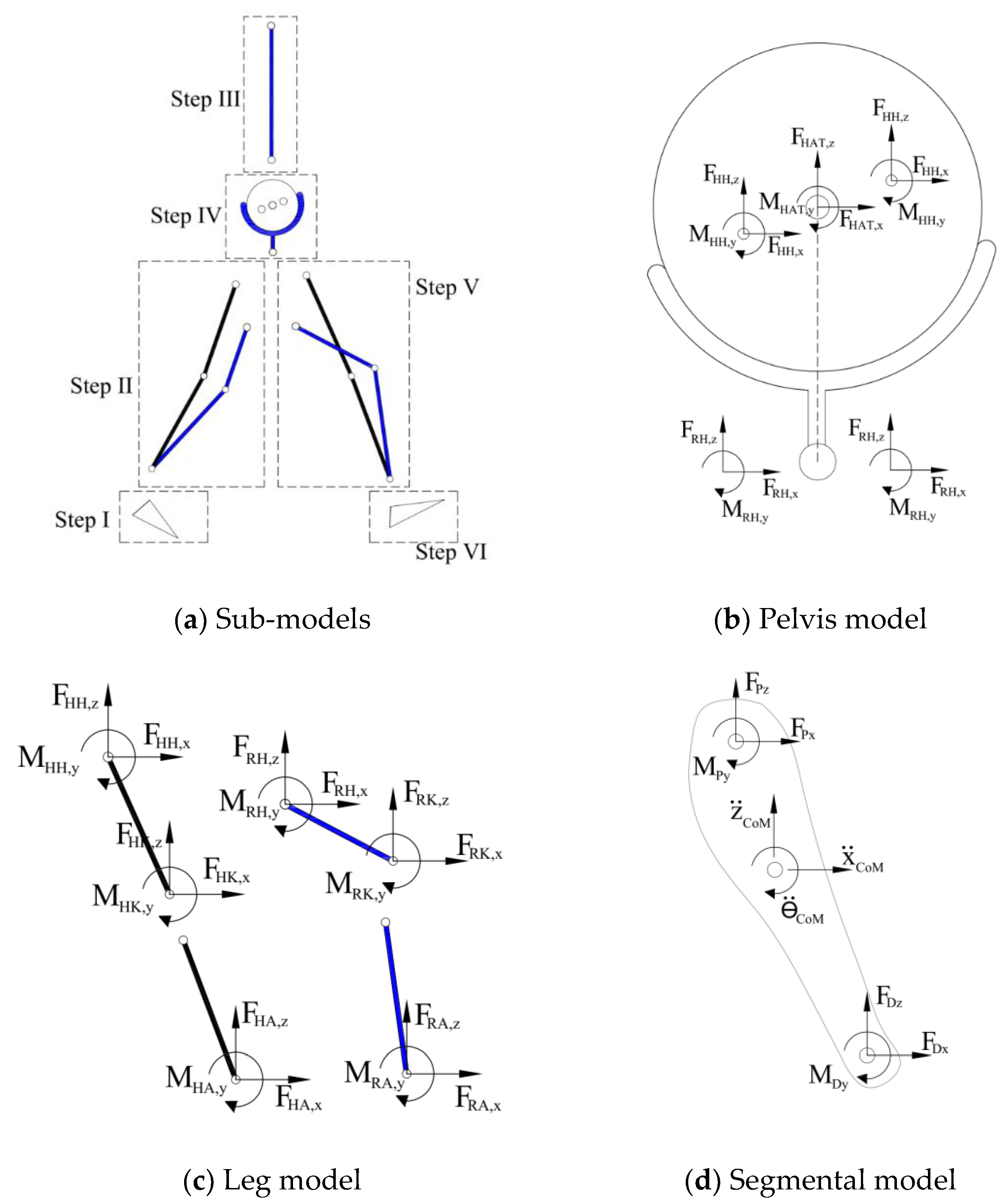
3. HRI Modelling Framework
- A.
- Human and robot are each modelled with an appropriate link segment (LS) model with lumped masses at each segment’s CoM and linked together based on the actual HRI configuration.
- B.
- Inverse Kinematics analysis is carried out to calculate the movements of human and robot segments from the measured marker trajectories.
- C.
- The contact forces between the human–robot system and the environment are estimated/measured.
- D.
- The system of equations of equilibrium for the human–robot LS model is formulated and solved for the net joint/interaction forces and torques (ID analysis). To make the system of equations statically determinate, the robot should have the same number of passive or active DoFs as the degree of indeterminacy of the human–robot system. Torque at each passive joint is set to zero. Assistive objectives of the robot are then used to define extra force/torque constraints, equal to the number of robot’s active DoFs, to make the system statically determinate.
4. Application of the HRI Framework to an Assistive Lower-Limb Exoskeleton
4.1. Step A
4.2. Step B
4.3. Step C
4.4. Steps D
5. Design Optimization
5.1. Center of Rotation of Hip Joint
5.2. Center of Rotation of Ankle Joint
5.3. Joint Torque–Velocity Requirements
6. Discussion and Conclusions
Author Contributions
Funding
Informed Consent Statement
Data Availability Statement
Conflicts of Interest
Nomenclature
| CDF | cumulative distribution function |
| CoM | center of mass |
| CoP | plantar center of pressure |
| D | distal |
| DoF | degree of freedom |
| DS | double-support phase of the walking gait |
| e | mean efficiency |
force (f) or moment (m) at
| |
| g | gravitational constant |
| GRF | ground reaction forces |
| HAT | head–arms–trunk |
| HRI | human–robot interaction |
| I | rotational inertia |
| ID | inverse dynamics |
| LS | link segment |
| m | mass |
| P | proximal |
| S | human subject |
| SS | single-support phase of the walking gait |
| walking speed | |
| w | walking |
References
- Hernandez, S.; Raison, M.; Baron, L.; Achiche, S. Refinement of Exoskeleton Design using Multibody Modeling: An Overview. In Proceedings of the CCToMM Mechanisms, Machines, and Mechatronics (M3) Symposium, Ottawa, ON, Canada, 28–29 May 2015. [Google Scholar]
- Sergi, F.; Accoto, D.; Tagliamonte, N.L.; Carpino, G.; Galzerano, S.; Guglielmelli, E. Kinematic synthesis, optimization and analysis of a non-anthropomorphic 2-DOFs wearable orthosis for gait assistance. In Proceedings of the 2012 IEEE/RSJ International Conference on Intelligent Robots and Systems (IROS 2012), Vilamoura-Algarve, Portugal, 7–12 October 2012; pp. 4303–4308. [Google Scholar]
- Accoto, D.; Sergi, F.; Tagliamonte, N.L.; Carpino, G.; Sudano, A.; Guglielmelli, E. Robomorphism: A Nonanthropomorphic Wearable Robot. IEEE Robot. Autom. Mag. 2014, 21, 45–55. [Google Scholar] [CrossRef]
- Ferrati, F.; Bortoletto, R.; Pagello, E. Virtual Modelling of a Real Exoskeleton Constrained to a Human Musculoskeletal Model. In Biomimetic and Biohybrid Systems; Lepora, N.F., Mura, A., Krapp, H.G., Verschure, P.F.M.J., Prescott, T.J., Eds.; Living Machines Lecture Notes in Computer Science; Springer: Berlin/Heidelberg, Germany, 2013; Volume 8064. [Google Scholar] [CrossRef]
- Agarwal, P.; Kuo, P.-H.; Neptune, R.R.; Deshpande, A.D. A Novel Framework for Virtual Prototyping of Rehabilitation Exoskeletons. In Proceedings of the 2013 IEEE 13th International Conference on Rehabilitation Robotics (ICORR 2013), Seattle, WA, USA, 24–26 June 2013; pp. 1–6. [Google Scholar]
- Galinski, D.; Sapin, J.; Dehez, B. Optimal design of an alignment-free two-DOF rehabilitation robot for the shoulder complex. In Proceedings of the 2013 IEEE 13th International Conference on Rehabilitation Robotics (ICORR 2013), Seattle, WA, USA, 24–26 June 2013; pp. 1–7. [Google Scholar]
- Shourijeh, M.; Jung, M.; Damsgaard, M. Metabolic Energy Consumption in a Box-Lifting Task: A Parametric Study on the Assistive Torque. In Biosystems & Biorobotics; Springer: Berlin/Heidelberg, Germany; pp. 143–148. [CrossRef]
- de Kruif, B.J.; Schmidhauser, E.; Stadler, K.S.; O’sullivan, L.W. Simulation Architecture for Modelling Interaction Between User and Elbow-articulated Exoskeleton. J. Bionic Eng. 2017, 14, 706–715. [Google Scholar] [CrossRef]
- Fournier, B.N.; Lemaire, E.D.; Smith, A.J.J.; Doumit, M. Modeling and Simulation of a Lower Extremity Powered Exoskeleton. IEEE Trans. Neural Syst. Rehabilitation Eng. 2018, 26, 1596–1603. [Google Scholar] [CrossRef] [PubMed]
- Zhou, L.; Li, Y.; Bai, S. A human-centered design optimization approach for robotic exoskeletons through biomechanical simulation. Robot. Auton. Syst. 2017, 91, 337–347. [Google Scholar] [CrossRef]
- Kim, H.; Miller, L.M.; Byl, N.; Abrams, G.M.; Rosen, J. Redundancy resolution of the human arm and an upper limb exoskeleton. IEEE Trans. Biomed. Eng. 2012, 59, 1770–1779. [Google Scholar] [CrossRef] [PubMed]
- Manns, P.; Sreenivasa, M.; Millard, M.; Mombaur, K. Motion Optimization and Parameter Identification for a Human and Lower Back Exoskeleton Model. IEEE Robot. Autom. Lett. 2017, 2, 1564–1570. [Google Scholar] [CrossRef]
- Vantilt, J.; Tanghe, K.; Afschrift, M.; Bruijnes, A.K.; Junius, K.; Geeroms, J.; Aertbeliën, E.; De Groote, F.; Lefeber, D.; Jonkers, I.; et al. Model-based control for exoskeletons with series elastic actuators evaluated on sit-to-stand movements. J. Neuroeng. Rehabil. 2019, 16, 65. [Google Scholar] [CrossRef] [PubMed]
- Huang, R.; Cheng, H.; Qiu, J.; Zhang, J. Learning Physical Human–Robot Interaction With Coupled Cooperative Primitives for a Lower Exoskeleton. IEEE Trans. Autom. Sci. Eng. 2019, 16, 1566–1574. [Google Scholar] [CrossRef]
- Serrancoli, G.; Falisse, A.; Dembia, C.; Vantilt, J.; Tanghe, K.; Lefeber, D.; Jonkers, I.; De Schutter, J.; De Groote, F. Subject-Exoskeleton Contact Model Calibration Leads to Accurate Interaction Force Predictions. IEEE Trans. Neural Syst. Rehabil. Eng. 2019, 27, 1597–1605. [Google Scholar] [CrossRef] [PubMed]
- Shahabpoor, E.; Pavic, A. Estimation of Tri-Axial Walking Ground Reaction Forces of Left and Right Foot from Total Forces in Real-Life Environments. Sensors 2018, 18, 1966. [Google Scholar] [CrossRef] [PubMed]
- Sun, Y.; Hu, J.; Huang, R. Negative-Stiffness Structure Vibration-Isolation Design and Impedance Control for a Lower Limb Exoskeleton Robot. Actuators 2023, 12, 147. [Google Scholar] [CrossRef]
- Sun, Y.; Peng, Z.; Hu, J.; Ghosh, B.K. Event-triggered critic learning impedance control of lower limb exoskeleton robots in interactive environments. Neurocomputing 2024, 564, 126963. [Google Scholar] [CrossRef]
- Shahabpoor, E.; Pavic, A.; Brownjohn, J.M.W.; Billings, S.A.; Guo, L.-Z.; Bocian, M. Real-Life Measurement of Tri-Axial Walking Ground Reaction Forces Using Optimal Network of Wearable Inertial Measurement Units. IEEE Trans. Neural Syst. Rehabil. Eng. 2018, 26, 1243–1253. [Google Scholar] [CrossRef] [PubMed]
- Charnwood Dynamics Limited, Coda Motion Capture System. Available online: https://codamotion.com/complete-movement-analysis-systems/ (accessed on 22 June 2024).
- Vicon Motion Systems, Bonita Motion Capture System Data Sheet. Available online: https://www.vicon.com/file/vicon/bonita-brochure.pdf (accessed on 28 October 2016).
- MathWorks, MATLAB and Statistics Toolbox Release Natick, MA, USA. Available online: https://www.scirp.org/reference/referencespapers?referenceid=2052124 (accessed on 18 June 2024).
- Zijlstra, W. Assessment of spatio-temporal parameters during unconstrained walking. Eur. J. Appl. Physiol. 2004, 92, 39–44. [Google Scholar] [CrossRef] [PubMed]
- Ren, L.; Jones, R.K.; Howard, D. Whole body inverse dynamics over a complete gait cycle based only on measured kinematics. J. Biomech. 2008, 41, 2750–2759. [Google Scholar] [CrossRef] [PubMed]
- Winter, D.A. The Biomechanics and Motor Control of Human Gait: Normal, Elderly and Pathological; University of Waterloo Press: Waterloo, ON, Canada, 1991. [Google Scholar]
- Stienen, A.H.A.; Hekman, E.E.G.; van der Helm, F.C.T.; van der Kooij, H. Self-Aligning Exoskeleton Axes through Decoupling of Joint Rotations and Translations. IEEE Trans. Robot. 2009, 25, 628–633. [Google Scholar] [CrossRef]
- Fuchioka, S.; Iwata, A.; Higuchi, Y.; Miyake, M.; Kanda, S.; Nishiyama, T. The Forward Velocity of the Center of Pressure in the Midfoot is a Major Predictor of Gait Speed in Older Adults. Int. J. Gerontol. 2015, 9, 119–122. [Google Scholar] [CrossRef]
- Wang, Y.; Wong, D.W.-C.; Tan, Q.; Li, Z.; Zhang, M. Total ankle arthroplasty and ankle arthrodesis affect the biomechanics of the inner foot differently. Sci. Rep. 2019, 9, 13334. [Google Scholar] [CrossRef] [PubMed]
- Maxon Group, EC 90 Flat 600 W Catalogue. Available online: https://www.maxongroup.co.uk/medias/sys_master/root/8882567643166/EN-21-312.pdf (accessed on 10 November 2021).


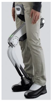
 |  | Honda walking assist: 1 active DoF per leg: hip 15 unknowns and 15 equations and constraints In each leg link segment model:
|
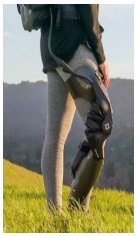 |  | Ascend robotic knee brace (Roam Robotics): 1 active DoF per leg: knee 18 unknowns and 18 equations and constraints In each leg link segment model:
|
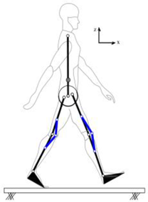
 |  | Fall prevention robot developed by the authors: 1 active DoF per leg: hip 15 unknowns and 15 equations and constraints In each leg link segment model:
|
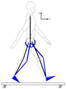
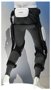 |  | Samsung walking assist robot: 2 active DoFs per leg: hip and knee 18 unknowns and 18 equations and constraints In each leg link segment model:
|
 |  | Honda weight support robot: 1 active DoFs per leg: knee 18 unknowns and 18 equations and constraints In each leg link segment model:
|
Conf (a) | Conf (b) | Conf (c) | Conf (a) | Conf (b) | Conf (c) | |
|---|---|---|---|---|---|---|
| 92% | 97% | 99% | 68% | 73% | 80% |
Unassisted | Conf (a) | Conf (b) | Conf (c) | Conf (a) | Conf (b) | Conf (c) | |
|---|---|---|---|---|---|---|---|
| 0.09 | 0.10 | 0.12 | 0.16 | 0.09 | 0.07 | 0.10 | |
| 0.028 | 0.025 | 0.032 | 0.038 | 0.028 | 0.022 | 0.023 |
Disclaimer/Publisher’s Note: The statements, opinions and data contained in all publications are solely those of the individual author(s) and contributor(s) and not of MDPI and/or the editor(s). MDPI and/or the editor(s) disclaim responsibility for any injury to people or property resulting from any ideas, methods, instructions or products referred to in the content. |
© 2024 by the authors. Licensee MDPI, Basel, Switzerland. This article is an open access article distributed under the terms and conditions of the Creative Commons Attribution (CC BY) license (https://creativecommons.org/licenses/by/4.0/).
Share and Cite
Shahabpoor, E.; Gray, B.; Plummer, A. Wearable Robot Design Optimization Using Closed-Form Human–Robot Dynamic Interaction Model. Sensors 2024, 24, 4081. https://doi.org/10.3390/s24134081
Shahabpoor E, Gray B, Plummer A. Wearable Robot Design Optimization Using Closed-Form Human–Robot Dynamic Interaction Model. Sensors. 2024; 24(13):4081. https://doi.org/10.3390/s24134081
Chicago/Turabian StyleShahabpoor, Erfan, Bethany Gray, and Andrew Plummer. 2024. "Wearable Robot Design Optimization Using Closed-Form Human–Robot Dynamic Interaction Model" Sensors 24, no. 13: 4081. https://doi.org/10.3390/s24134081
APA StyleShahabpoor, E., Gray, B., & Plummer, A. (2024). Wearable Robot Design Optimization Using Closed-Form Human–Robot Dynamic Interaction Model. Sensors, 24(13), 4081. https://doi.org/10.3390/s24134081