
LidPose: Real-Time 3D Human Pose Estimation in Sparse Lidar Point Clouds with Non-Repetitive Circular Scanning Pattern


Abstract
1. Introduction
1.1. Related Works
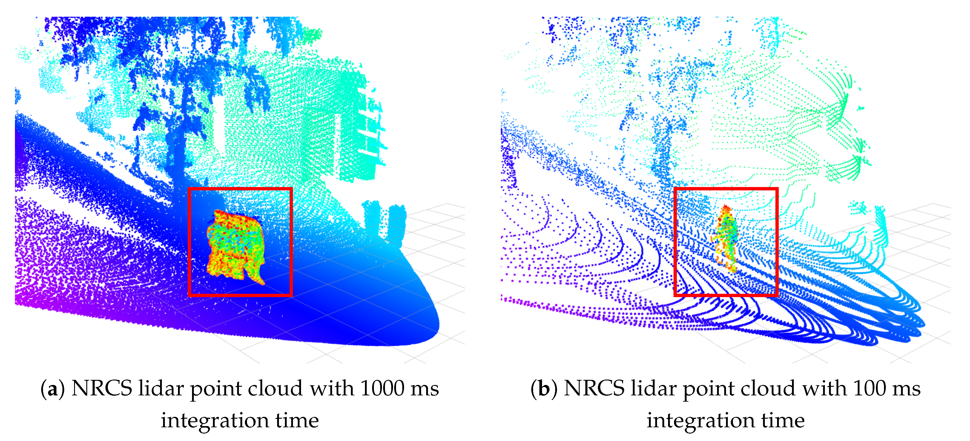
1.2. NRCS Lidar Sensor
1.3. Contributions and Paper Outline
- We propose a novel, real-time, end-to-end 3D human pose estimation method using only sparse NRCS lidar point clouds.
- A new dataset is created including synchronized and calibrated lidar and camera data along with human pose annotations. Note that in our lidar-only approach, camera images are only used for parameter training and validation of the results.
- Using this dataset, we demonstrate in multiple experiments the proper input data and network architecture to achieve accurate and real-time 3D human pose estimation in NRCS lidar point clouds.
2. Proposed Method
2.1. ViTPose
2.2. LidPose
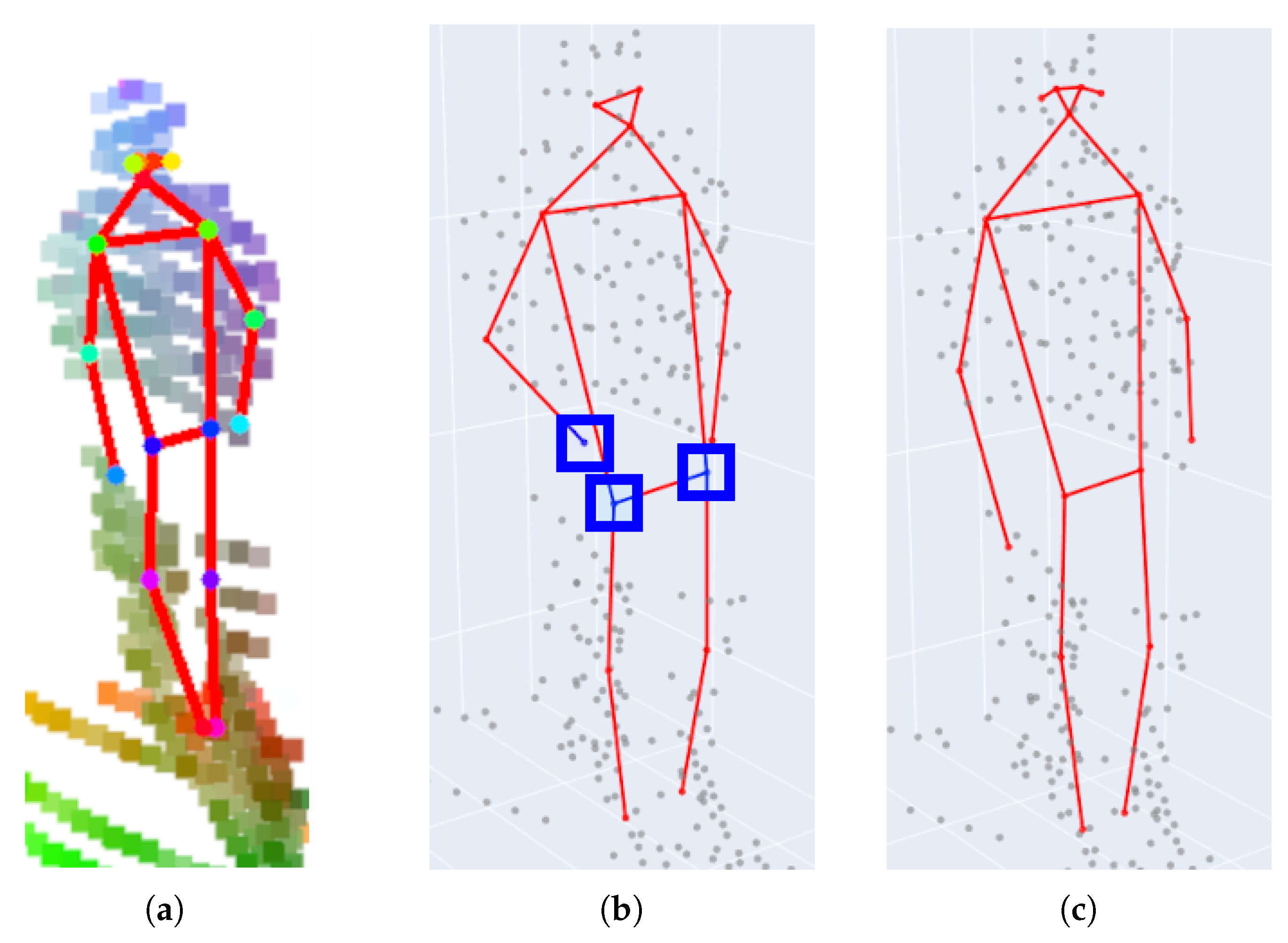
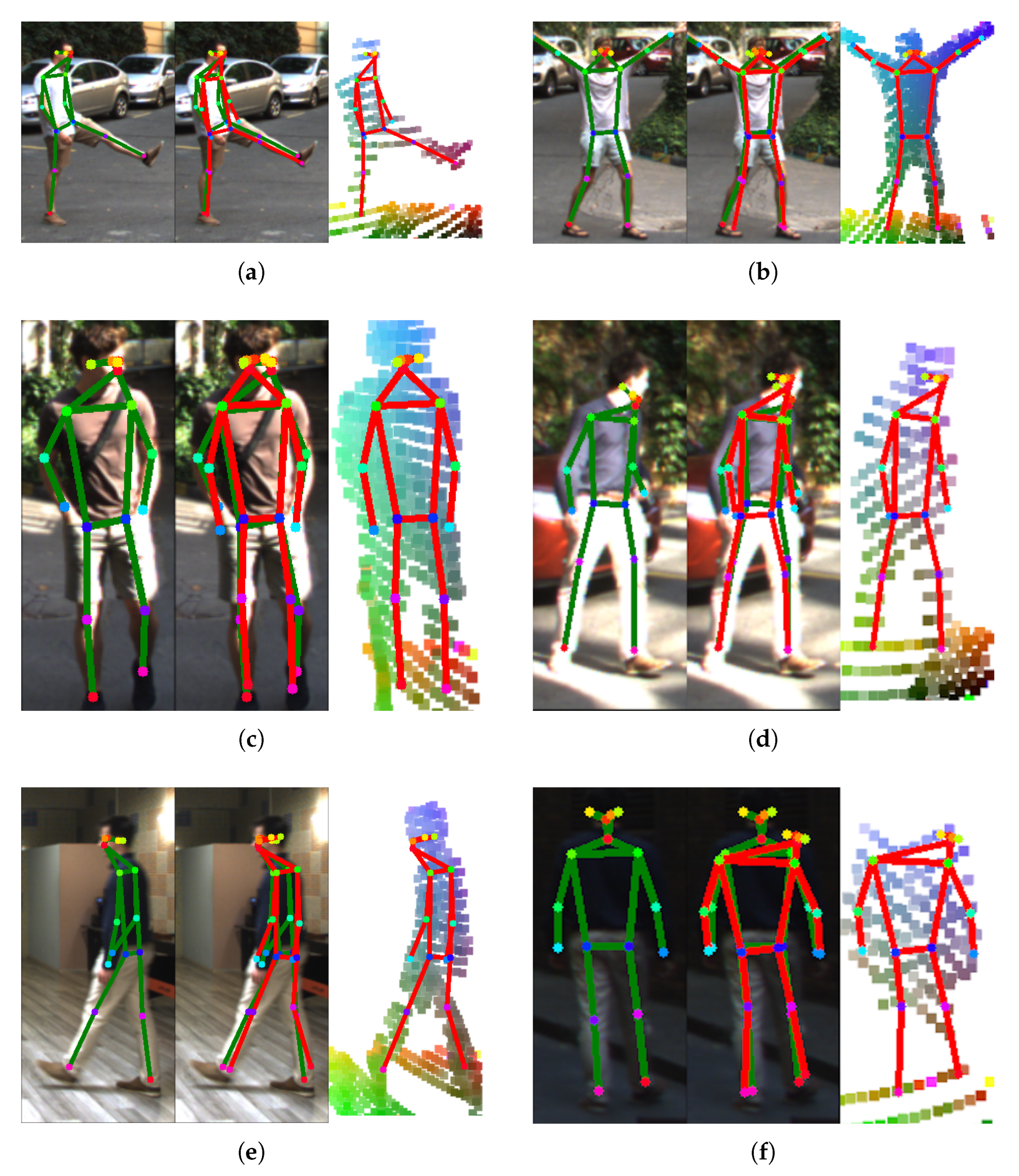
- LidPose–2D predicts the human poses in the 2D domain, i.e., it detects the projections of the joints (i.e., skeleton keypoints) onto the pixel lattice of the range images, as shown in Figure 4a. While this approach can lead to robust 2D pose detection, it does not predict the depth information of the joint positions.
- LidPose–2D+ extends the result of the LidPose–2D prediction to 3D for those joints, where valid values exist in the range image representation of the lidar point cloud, as shown in Figure 4b. This serves as the baseline of the 3D prediction, with a limitation that due to the sparsity of the lidar range measurements, some joints will not be associated with valid depth values (marked by blue boxes in Figure 4b).
- LidPose–3D is the extended version of LidPose–2D+, where depth values are estimated for all joints based on a training step. This approach predicts the 3D human poses in the world coordinate system from the sparse input lidar point cloud, as shown in Figure 4c.
- A new patch-embedding implementation was applied to the network backbone to handle efficiently and dynamically the different input channel counts.
- The number of transformer blocks used in the LidPose backbone was increased to enhance the network’s generalization capabilities by having more parameters.
- The output of the LidPose–3D configuration was modified as well by extending the predictions’ dimensions to be able to predict the joint depths alongside the 2D predictions.
- Depth only (D);
- 3D coordinates only (XYZ);
- 3D + depth (XYZ+D);
- 3D + intensity (XYZ+I);
- 3D + depth + intensity (XYZ+D+I).
2.2.1. LidPose–2D
2.2.2. LidPose–2D+
2.2.3. LidPose–3D
2.3. LidPose Training
3. Dataset for Lidar-Only 3D Human Pose Estimation
3.1. Spatio-Temporal Registration of Lidar and Camera Data
3.2. Human Pose Ground Truth
3.2.1. 2D Human Pose Ground Truth
3.2.2. 3D Human Pose Ground Truth
3.3. Transforming the Point Cloud to the Five-Channel Range Image Representation
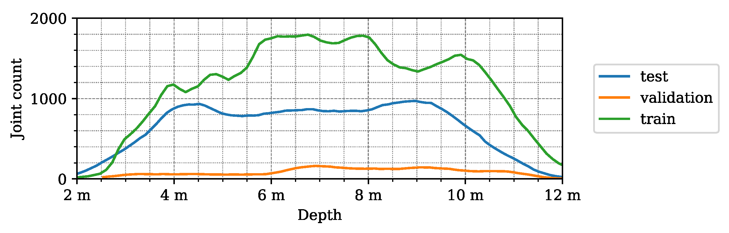
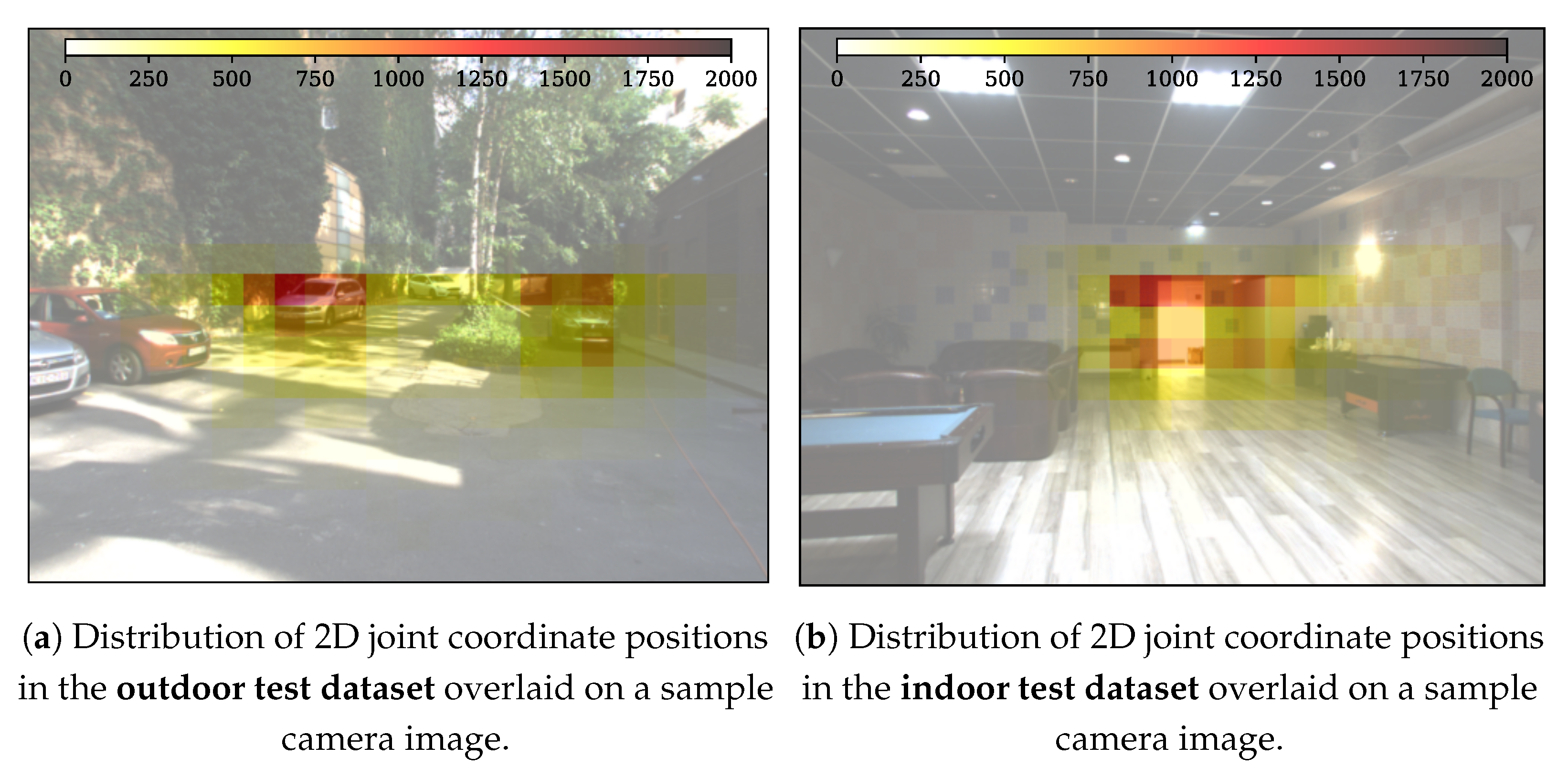
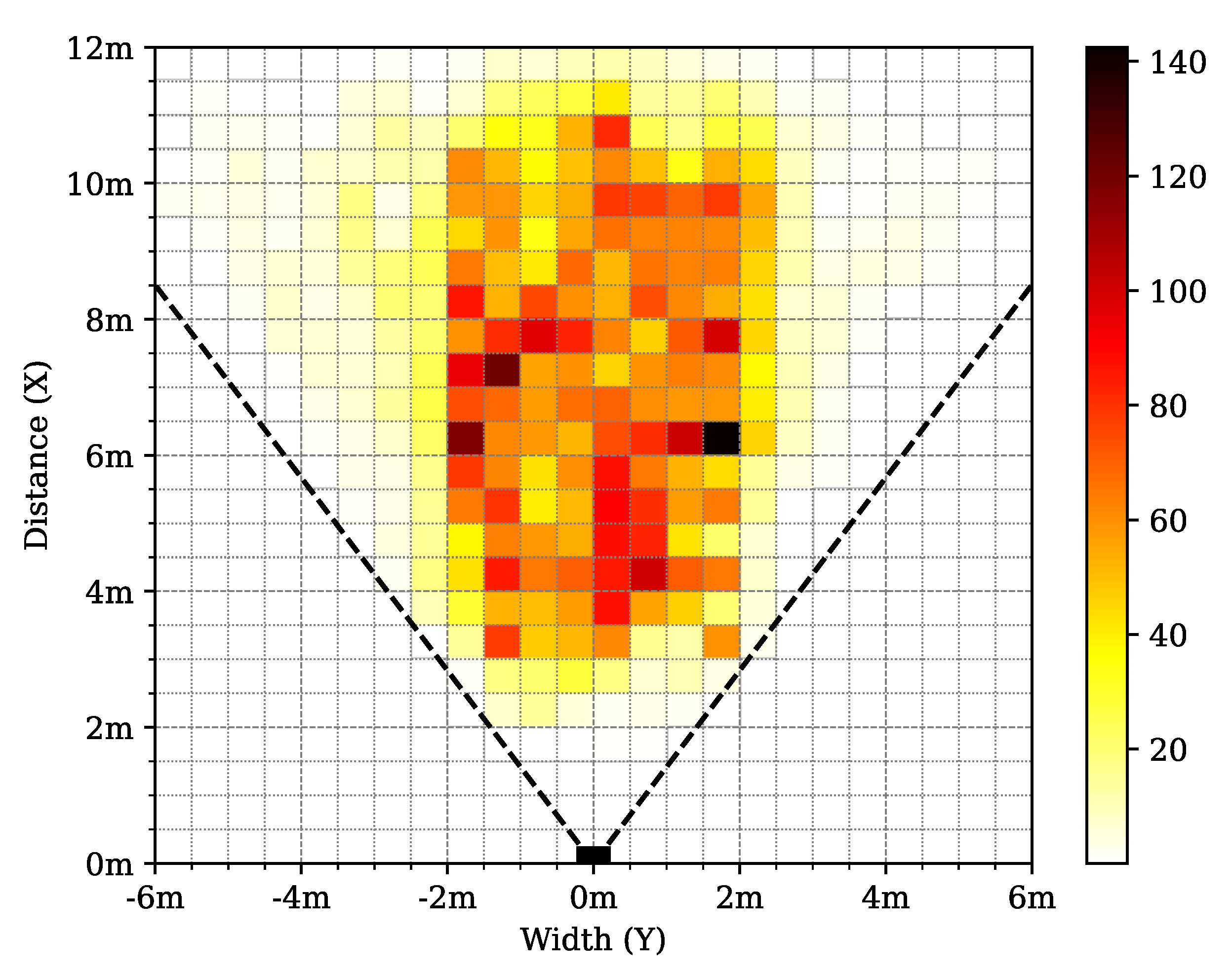
3.4. Dataset Parameters
4. Experiments and Results

| Model | Input | ADE ↓ | PCK ↑ | AUC-PCK ↑ | LAE ↓ | LLE ↓ |
|---|---|---|---|---|---|---|
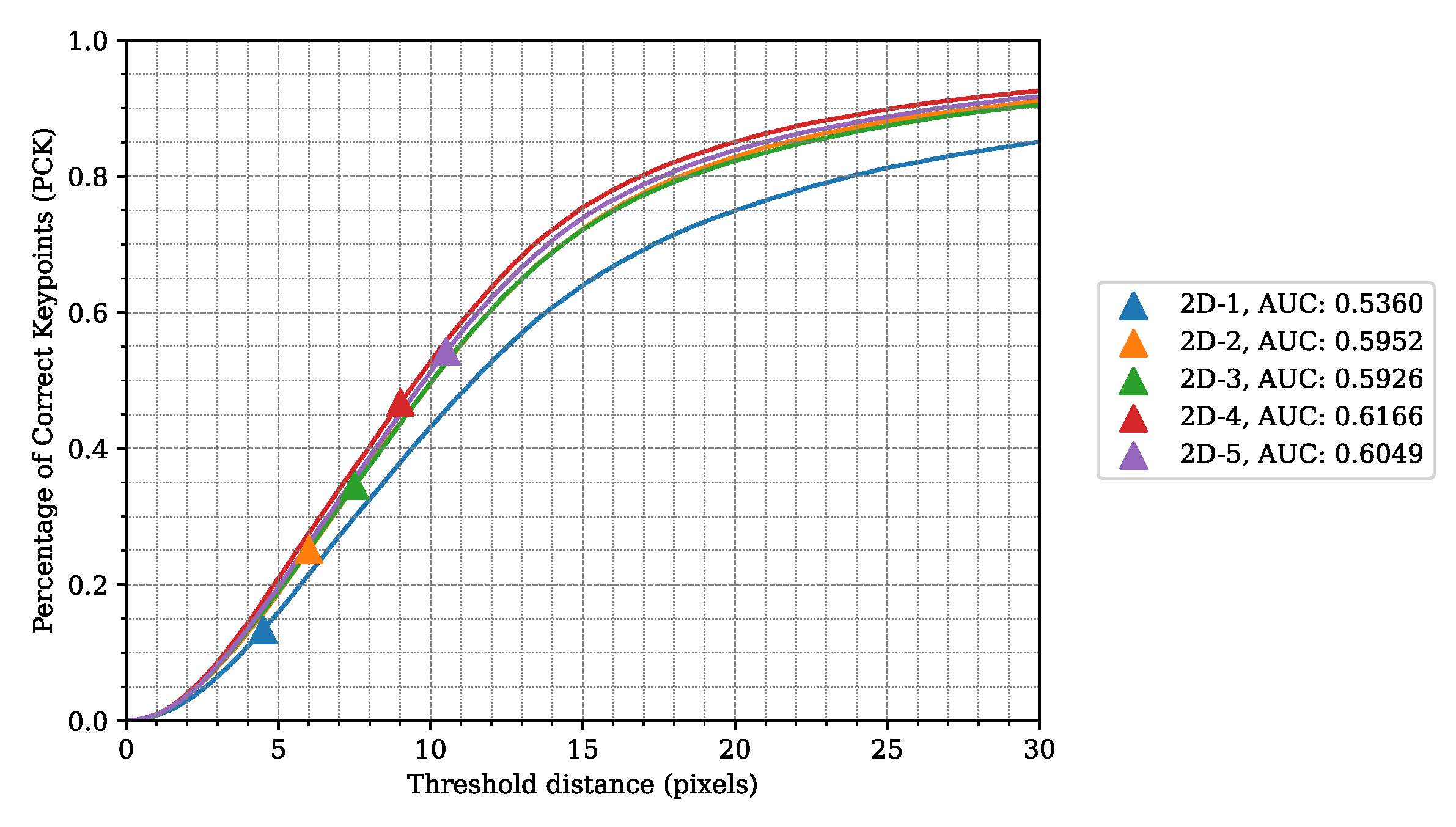
| 2D–1 | D | 18.0726 | 0.4316 | 0.5360 | 13.7856 | 9.7695 |
| 2D–2 | XYZ | 14.4013 | 0.4960 | 0.5952 | 12.6956 | 9.5330 |
| 2D–3 | XYZ+D | 14.6881 | 0.4966 | 0.5926 | 12.7078 | 9.4509 |
| 2D–4 | XYZ+I | 13.2473 | 0.5278 | 0.6166 | 12.5251 | 10.6579 |
| 2D–5 | XYZ+D+I | 13.8399 | 0.5122 | 0.6049 | 12.6762 | 11.1547 |
| Model | Head | Shoulders | Elbows | Wrists | Hips | Knees | Ankles | ADE ↓ |
|---|---|---|---|---|---|---|---|---|
| 2D–1 | 12.4838 | 17.5230 | 25.2190 | 27.6912 | 13.6437 | 16.6865 | 21.6442 | 18.0726 |
| 2D–2 | 11.3505 | 12.8925 | 17.3831 | 19.7888 | 10.9468 | 13.7076 | 19.3161 | 14.4013 |
| 2D–3 | 11.2303 | 13.1998 | 18.1070 | 20.5023 | 11.2541 | 14.0968 | 19.6134 | 14.6881 |
| 2D–4 | 10.0393 | 11.1264 | 14.5071 | 17.0304 | 11.5661 | 13.9160 | 19.3576 | 13.2473 |
| 2D–5 | 10.1436 | 11.6997 | 15.8984 | 18.6925 | 12.7537 | 14.1663 | 19.0698 | 13.8399 |
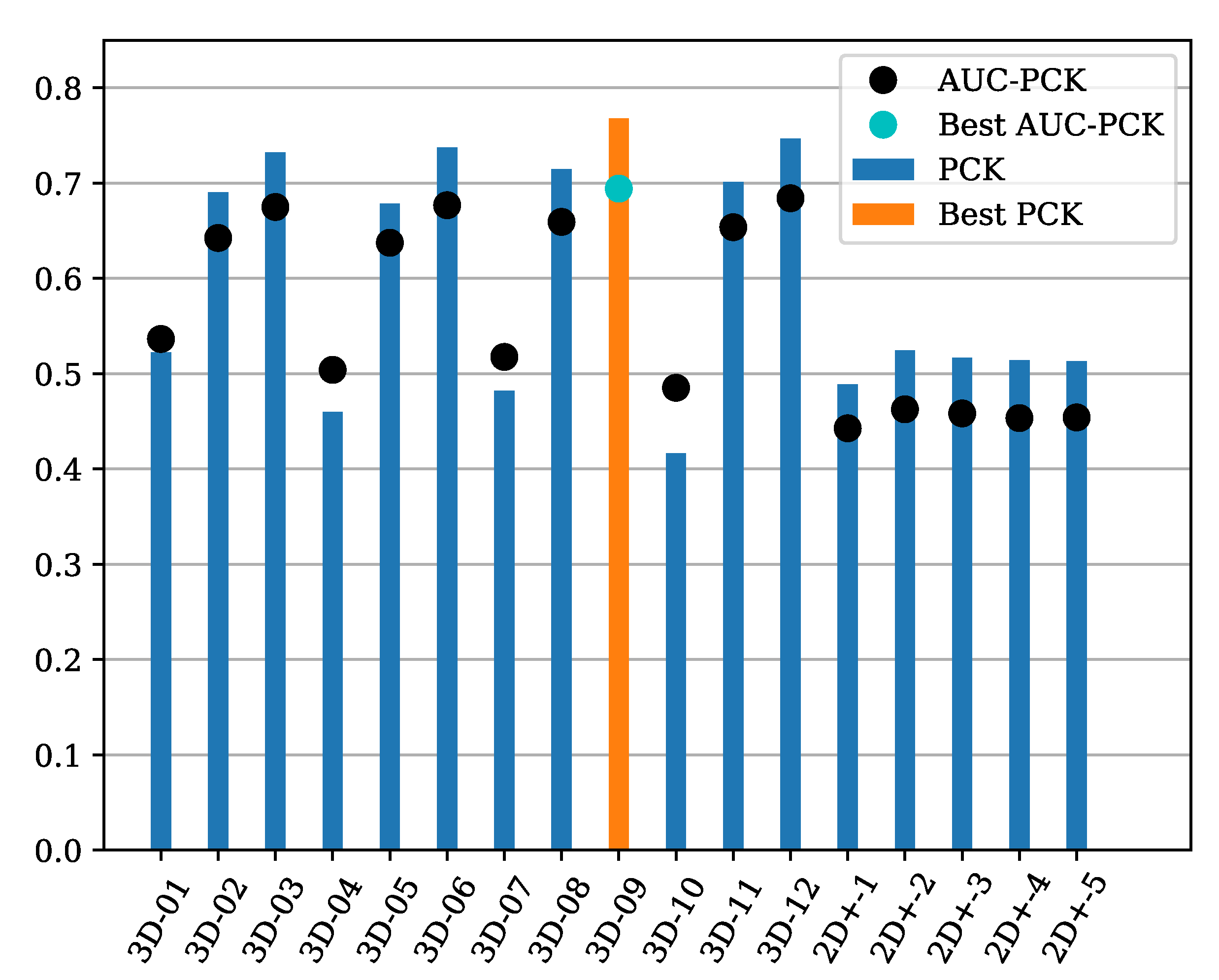
| Model | Input | Depth L. | ADE ↓ | PCK ↑ | AUC-PCK ↑ | LAE ↓ | LLE ↓ |
|---|---|---|---|---|---|---|---|
| 3D–01 | XYZ | L1 | 0.3372 | 0.5222 | 0.5364 | 22.5130 | 0.9247 |
| 3D–02 | XYZ | L2 | 0.1848 | 0.6904 | 0.6424 | 21.9994 | 0.0966 |
| 3D–03 | XYZ | SSIM | 0.1683 | 0.7322 | 0.6749 | 20.7884 | 0.0903 |
| 3D–04 | XYZ+D | L1 | 0.2679 | 0.4599 | 0.5040 | 24.8060 | 0.1868 |
| 3D–05 | XYZ+D | L2 | 0.1873 | 0.6784 | 0.6374 | 22.3703 | 0.0964 |
| 3D–06 | XYZ+D | SSIM | 0.1676 | 0.7374 | 0.6768 | 20.6084 | 0.0908 |
| 3D–07 | XYZ+I | L1 | 0.2576 | 0.4822 | 0.5176 | 25.0920 | 0.1769 |
| 3D–08 | XYZ+I | L2 | 0.1762 | 0.7147 | 0.6593 | 21.6107 | 0.1047 |
| 3D–09 | XYZ+I | SSIM | 0.1583 | 0.7678 | 0.6942 | 20.6737 | 0.0952 |
| 3D–10 | XYZ+D+I | L1 | 0.2764 | 0.4164 | 0.4852 | 31.0437 | 0.2274 |
| 3D–11 | XYZ+D+I | L2 | 0.1794 | 0.7014 | 0.6537 | 21.9404 | 0.1064 |
| 3D–12 | XYZ+D+I | SSIM | 0.1633 | 0.7466 | 0.6841 | 21.1505 | 0.0983 |
| 2D+–1 | D | - | 2.4477 | 0.4887 | 0.4427 | 32.4529 | 1.4299 |
| 2D+–2 | XYZ | - | 2.4758 | 0.5242 | 0.4626 | 32.5635 | 1.4419 |
| 2D+–3 | XYZ+D | - | 2.4910 | 0.5165 | 0.4583 | 33.3569 | 1.4723 |
| 2D+–4 | XYZ+I | - | 2.5901 | 0.5141 | 0.4534 | 34.0922 | 1.5538 |
| 2D+–5 | XYZ+D+I | - | 2.5671 | 0.5133 | 0.4541 | 33.5011 | 1.3705 |
4.1. Metrics
4.2. Experiment Parameters
4.3. LidPose–2D Evaluation
4.4. LidPose–3D Evaluation
5. Conclusions and Future Work
Author Contributions
Funding
Institutional Review Board Statement
Informed Consent Statement
Data Availability Statement
Acknowledgments
Conflicts of Interest
Abbreviations
| ADE | Average distance error |
| AUC | Area under curve |
| Bg | Background |
| COCO | Microsoft COCO: Common Objects in Context dataset |
| FFN | Feed-forward network |
| FoV | Field of view |
| FPS | Frames per second |
| GT | Ground truth |
| IMU | Inertial measurement unit |
| HUN-REN | Hungarian Research Network (https://hun-ren.hu/en) |
| LAE | Limb angle error |
| LLE | Limb length error |
| MHSA | Multi-head self-attention |
| MRF | Markov random fields |
| MoGs | Mixture of Gaussians |
| MPJPE | Mean per-joint position error |
| MSE | Mean squared error |
| NRCS | Non-repetitive circular scanning |
| PCK | Percentage of correct keypoints |
| PTPd | Precision Time Protocol daemon |
| ReLU | Rectified linear unit |
| RoI | Region of interest |
| RMB | Rotating multi-beam |
| SLAM | Simultaneous localization and mapping |
| SSIM | Structural similarity index measure |
References
- Zimmermann, C.; Welschehold, T.; Dornhege, C.; Burgard, W.; Brox, T. 3D Human Pose Estimation in RGBD Images for Robotic Task Learning. In Proceedings of the 2018 IEEE International Conference on Robotics and Automation (ICRA), Brisbane, QLD, Australia, 21–25 May 2018; pp. 1986–1992. [Google Scholar] [CrossRef]
- Cormier, M.; Clepe, A.; Specker, A.; Beyerer, J. Where are we with Human Pose Estimation in Real-World Surveillance? In Proceedings of the 2022 IEEE/CVF Winter Conference on Applications of Computer Vision Workshops (WACVW), Waikoloa, HI, USA, 4–8 January 2022; pp. 591–601. [Google Scholar] [CrossRef]
- Hu, W.; Tan, T.; Wang, L.; Maybank, S. A survey on visual surveillance of object motion and behaviors. IEEE Trans. Syst. Man Cybern. Part C (Appl. Rev.) 2004, 34, 334–352. [Google Scholar] [CrossRef]
- Zanfir, A.; Zanfir, M.; Gorban, A.; Ji, J.; Zhou, Y.; Anguelov, D.; Sminchisescu, C. HUM3DIL: Semi-supervised Multi-modal 3D Human Pose Estimation for Autonomous Driving. In Proceedings of the 6th Conference on Robot Learning, Auckland, New Zealand, 14–18 December 2022. [Google Scholar] [CrossRef]
- Rossol, N.; Cheng, I.; Basu, A. A Multisensor Technique for Gesture Recognition Through Intelligent Skeletal Pose Analysis. IEEE Trans.-Hum.-Mach. Syst. 2016, 46, 350–359. [Google Scholar] [CrossRef]
- Sharma, P.; Shah, B.B.; Prakash, C. A Pilot Study on Human Pose Estimation for Sports Analysis. In Proceedings of the Pattern Recognition and Data Analysis with Applications; Gupta, D., Goswami, R.S., Banerjee, S., Tanveer, M., Pachori, R.B., Eds.; Springer Nature: Singapore, 2022; pp. 533–544. [Google Scholar] [CrossRef]
- Chua, J.; Ong, L.Y.; Leow, M.C. Telehealth Using PoseNet-Based System for In-Home Rehabilitation. Future Internet 2021, 13, 173. [Google Scholar] [CrossRef]
- Rabosh, E.V.; Balbekin, N.S.; Timoshenkova, A.M.; Shlykova, T.V.; Petrov, N.V. Analog-to-digital conversion of information archived in display holograms: II. photogrammetric digitization. J. Opt. Soc. Am. A 2023, 40, B57–B64. [Google Scholar] [CrossRef] [PubMed]
- Nguyen, T.; Qui, T.; Xu, K.; Cheok, A.; Teo, S.; Zhou, Z.; Mallawaarachchi, A.; Lee, S.; Liu, W.; Teo, H.; et al. Real-time 3D human capture system for mixed-reality art and entertainment. IEEE Trans. Vis. Comput. Graph. 2005, 11, 706–721. [Google Scholar] [CrossRef] [PubMed]
- Livox Avia Specifications. Available online: https://www.livoxtech.com/avia/specs (accessed on 11 March 2024).
- Cao, Z.; Hidalgo, G.; Simon, T.; Wei, S.; Sheikh, Y. OpenPose: Realtime Multi-Person 2D Pose Estimation Using Part Affinity Fields. IEEE Trans. Pattern Anal. Mach. Intell. 2021, 43, 172–186. [Google Scholar] [CrossRef] [PubMed]
- Fang, H.S.; Li, J.; Tang, H.; Xu, C.; Zhu, H.; Xiu, Y.; Li, Y.L.; Lu, C. AlphaPose: Whole-Body Regional Multi-Person Pose Estimation and Tracking in Real-Time. IEEE Trans. Pattern Anal. Mach. Intell. 2023, 45, 7157–7173. [Google Scholar] [CrossRef] [PubMed]
- Lu, P.; Jiang, T.; Li, Y.; Li, X.; Chen, K.; Yang, W. RTMO: Towards High-Performance One-Stage Real-Time Multi-Person Pose Estimation. arXiv 2023, arXiv:2312.07526. [Google Scholar] [CrossRef]
- Zheng, J.; Shi, X.; Gorban, A.; Mao, J.; Song, Y.; Qi, C.R.; Liu, T.; Chari, V.; Cornman, A.; Zhou, Y.; et al. Multi-modal 3D Human Pose Estimation with 2D Weak Supervision in Autonomous Driving. arXiv 2021, arXiv:2112.12141. [Google Scholar] [CrossRef]
- Wang, K.; Xie, J.; Zhang, G.; Liu, L.; Yang, J. Sequential 3D Human Pose and Shape Estimation From Point Clouds. In Proceedings of the 2020 IEEE/CVF Conference on Computer Vision and Pattern Recognition (CVPR), Seattle, WA, USA, 13–19 June 2020; pp. 7273–7282. [Google Scholar] [CrossRef]
- Ren, Y.; Han, X.; Zhao, C.; Wang, J.; Xu, L.; Yu, J.; Ma, Y. LiveHPS: LiDAR-based Scene-level Human Pose and Shape Estimation in Free Environment. arXiv 2024, arXiv:2402.17171. [Google Scholar] [CrossRef]
- Ren, Y.; Zhao, C.; He, Y.; Cong, P.; Liang, H.; Yu, J.; Xu, L.; Ma, Y. LiDAR-aid Inertial Poser: Large-scale Human Motion Capture by Sparse Inertial and LiDAR Sensors. IEEE Trans. Vis. Comput. Graph. 2023, 29, 2337–2347. [Google Scholar] [CrossRef] [PubMed]
- Zhou, Y.; Dong, H.; Saddik, A.E. Learning to Estimate 3D Human Pose From Point Cloud. IEEE Sens. J. 2020, 20, 12334–12342. [Google Scholar] [CrossRef]
- Zhang, M.; Cui, Z.; Neumann, M.; Chen, Y. An End-to-End Deep Learning Architecture for Graph Classification. In Proceedings of the AAAI Conference on Artificial Intelligence, New Orleans, LA, USA, 2–7 February 2018; Volume 32. [Google Scholar] [CrossRef]
- Ye, D.; Xie, Y.; Chen, W.; Zhou, Z.; Ge, L.; Foroosh, H. LPFormer: LiDAR Pose Estimation Transformer with Multi-Task Network. arXiv 2024, arXiv:2306.12525. [Google Scholar] [CrossRef]
- Sun, P.; Kretzschmar, H.; Dotiwalla, X.; Chouard, A.; Patnaik, V.; Tsui, P.; Guo, J.; Zhou, Y.; Chai, Y.; Caine, B.; et al. Scalability in Perception for Autonomous Driving: Waymo Open Dataset. In Proceedings of the IEEE/CVF Conference on Computer Vision and Pattern Recognition (CVPR), Seattle, WA, USA, 13–19 June 2020. [Google Scholar] [CrossRef]
- Vaswani, A.; Shazeer, N.; Parmar, N.; Uszkoreit, J.; Jones, L.; Gomez, A.N.; Kaiser, L.u.; Polosukhin, I. Attention is All you Need. In Proceedings of the 31st International Conference on Neural Information Processing Systems, Long Beach, CA, USA, 4–9 December 2017; Curran Associates Inc.: Red Hook, NY, USA, 2017; Volume 30. [Google Scholar]
- Dosovitskiy, A.; Beyer, L.; Kolesnikov, A.; Weissenborn, D.; Zhai, X.; Unterthiner, T.; Dehghani, M.; Minderer, M.; Heigold, G.; Gelly, S.; et al. An Image is Worth 16x16 Words: Transformers for Image Recognition at Scale. arXiv 2021, arXiv:2010.11929. [Google Scholar] [CrossRef]
- Carion, N.; Massa, F.; Synnaeve, G.; Usunier, N.; Kirillov, A.; Zagoruyko, S. End-to-End Object Detection with Transformers. arXiv 2020, arXiv:2005.12872. [Google Scholar] [CrossRef]
- Parmar, N.J.; Vaswani, A.; Uszkoreit, J.; Kaiser, L.; Shazeer, N.; Ku, A.; Tran, D. Image Transformer. In Proceedings of the International Conference on Machine Learning (ICML), Stockholm, Sweden, 10–15 July 2018. [Google Scholar] [CrossRef]
- Zhang, B.; Gu, S.; Zhang, B.; Bao, J.; Chen, D.; Wen, F.; Wang, Y.; Guo, B. StyleSwin: Transformer-based GAN for High-resolution Image Generation. arXiv 2022, arXiv:2112.10762. [Google Scholar] [CrossRef]
- Chang, H.; Zhang, H.; Jiang, L.; Liu, C.; Freeman, W.T. MaskGIT: Masked Generative Image Transformer. In Proceedings of the IEEE Conference on Computer Vision and Pattern Recognition (CVPR), New Orleans, LA, USA, 18–24 June 2022. [Google Scholar] [CrossRef]
- Xu, Y.; Zhang, J.; Zhang, Q.; Tao, D. ViTPose: Simple Vision Transformer Baselines for Human Pose Estimation. In Proceedings of the Advances in Neural Information Processing Systems; Curran Associates, Inc.: Red Hook, NY, USA, 2022; Volume 35, pp. 38571–38584. [Google Scholar] [CrossRef]
- Stoffl, L.; Vidal, M.; Mathis, A. End-to-end trainable multi-instance pose estimation with transformers. arXiv 2021, arXiv:2103.12115. [Google Scholar] [CrossRef]
- Toshev, A.; Szegedy, C. DeepPose: Human Pose Estimation via Deep Neural Networks. In Proceedings of the 2014 IEEE Conference on Computer Vision and Pattern Recognition, Columbus, OH, USA, 23–28 June 2014; pp. 1653–1660. [Google Scholar] [CrossRef]
- Xiao, B.; Wu, H.; Wei, Y. Simple Baselines for Human Pose Estimation and Tracking. In Proceedings of the Computer Vision—ECCV 2018, Munich, Germany, 8–14 September 2018; pp. 472–487. [Google Scholar] [CrossRef]
- Sun, K.; Xiao, B.; Liu, D.; Wang, J. Deep High-Resolution Representation Learning for Human Pose Estimation. In Proceedings of the 2019 IEEE/CVF Conference on Computer Vision and Pattern Recognition (CVPR), Long Beach, CA, USA, 15–20 June 2019; pp. 5686–5696. [Google Scholar] [CrossRef]
- Livox Avia User Manual. Available online: https://www.livoxtech.com/avia/downloads (accessed on 11 March 2024).
- Benedek, C.; Majdik, A.; Nagy, B.; Rozsa, Z.; Sziranyi, T. Positioning and perception in LIDAR point clouds. Digit. Signal Process. 2021, 119, 103193. [Google Scholar] [CrossRef]
- Heinzler, R.; Piewak, F.; Schindler, P.; Stork, W. CNN-Based Lidar Point Cloud De-Noising in Adverse Weather. IEEE Robot. Autom. Lett. 2020, 5, 2514–2521. [Google Scholar] [CrossRef]
- Lin, J.; Zhang, F. Loam livox: A fast, robust, high-precision LiDAR odometry and mapping package for LiDARs of small FoV. In Proceedings of the IEEE International Conference on Robotics and Automation (ICRA), Paris, France, 31 May–31 August 2020; pp. 3126–3131. [Google Scholar] [CrossRef]
- Wang, Y.; Lou, Y.; Zhang, Y.; Song, W.; Huang, F.; Tu, Z. A Robust Framework for Simultaneous Localization and Mapping with Multiple Non-Repetitive Scanning Lidars. Remote Sens. 2021, 13, 2015. [Google Scholar] [CrossRef]
- Glennie, C.L.; Hartzell, P.J. Accuracy assessment and calibration of low-cost autonomous sensors. Int. Arch. Photogramm. Remote Sens. Spat. Inf. Sci. 2020, XLIII-B1-2020, 371–376. [Google Scholar] [CrossRef]
- Kovács, L.; Kégl, M.; Benedek, C. Real-Time Foreground Segmentation for Surveillance Applications in NRCS Lidar Sequences. Int. Arch. Photogramm. Remote Sens. Spat. Inf. Sci. 2022, XLIII-B1-2022, 45–51. [Google Scholar] [CrossRef]
- Nagy, B.; Kovács, L.; Benedek, C. ChangeGAN: A Deep Network for Change Detection in Coarsely Registered Point Clouds. IEEE Robot. Autom. Lett. 2021, 6, 8277–8284. [Google Scholar] [CrossRef]
- Lin, T.Y.; Maire, M.; Belongie, S.; Bourdev, L.; Girshick, R.; Hays, J.; Perona, P.; Ramanan, D.; Zitnick, C.L.; Dollár, P. Microsoft COCO: Common Objects in Context. In Proceedings of the Computer Vision—ECCV 2014, Zurich, Switzerland, 6–12 September 2014; pp. 740–755. [Google Scholar] [CrossRef]
- Stauffer, C.; Grimson, W.E.L. Learning Patterns of Activity Using Real-Time Tracking. IEEE Trans. Pattern Anal. Mach. Intell. 2000, 22, 747–757. [Google Scholar] [CrossRef]
- Benedek, C. 3D people surveillance on range data sequences of a rotating Lidar. Pattern Recognit. Lett. 2014, 50, 149–158. [Google Scholar] [CrossRef]
- Wang, Z.; Bovik, A.; Sheikh, H.; Simoncelli, E. Image quality assessment: From error visibility to structural similarity. IEEE Trans. Image Process. 2004, 13, 600–612. [Google Scholar] [CrossRef]
- Bradski, G. The OpenCV Library. Dr. Dobb’s J. Softw. Tools 2000, 25, 120–123. [Google Scholar]
- OpenCV. The OpenCV Reference Manual, 4.9.0 ed. 2014. Available online: https://docs.opencv.org/4.9.0/ (accessed on 13 May 2024).
- Yuan, C.; Liu, X.; Hong, X.; Zhang, F. Pixel-level Extrinsic Self Calibration of High Resolution LiDAR and Camera in Targetless Environments. arXiv 2021, arXiv:2103.01627. [Google Scholar] [CrossRef]
- Eidson, J.C.; Fischer, M.; White, J. IEEE-1588™ Standard for a precision clock synchronization protocol for networked measurement and control systems. In Proceedings of the 34th Annual Precise Time and Time Interval Systems and Applications Meeting, Reston, VA, USA, 3–5 December 2002; pp. 243–254. [Google Scholar]
- Lao, K.; Yan, G. Implementation and Analysis of IEEE 1588 PTP Daemon Based on Embedded System. In Proceedings of the 2020 39th Chinese Control Conference (CCC), Shenyang, China, 27–29 July 2020; pp. 4377–4382. [Google Scholar] [CrossRef]
- Jocher, G.; Chaurasia, A.; Qiu, J. Ultralytics YOLOv8. 2023. Available online: https://github.com/ultralytics/ultralytics (accessed on 13 May 2024).
- Xu, Y.; Zhang, J.; Zhang, Q.; Tao, D. ViTPose: Simple Vision Transformer Baselines for Human Pose Estimation. 2022. Available online: https://github.com/ViTAE-Transformer/ViTPose (accessed on 13 May 2024).
- Pavllo, D.; Feichtenhofer, C.; Grangier, D.; Auli, M. 3D human pose estimation in video with temporal convolutions and semi-supervised training. In Proceedings of the Conference on Computer Vision and Pattern Recognition (CVPR), Long Beach, CA, USA, 15–20 June 2019. [Google Scholar] [CrossRef]
- Wu, Z.; Hoang, D.; Lin, S.Y.; Xie, Y.; Chen, L.; Lin, Y.Y.; Wang, Z.; Fan, W. MM-Hand: 3D-Aware Multi-Modal Guided Hand Generative Network for 3D Hand Pose Synthesis. arXiv 2020, arXiv:2010.01158. [Google Scholar] [CrossRef]
- Munea, T.L.; Jembre, Y.Z.; Weldegebriel, H.T.; Chen, L.; Huang, C.; Yang, C. The Progress of Human Pose Estimation: A Survey and Taxonomy of Models Applied in 2D Human Pose Estimation. IEEE Access 2020, 8, 133330–133348. [Google Scholar] [CrossRef]
- Héder, M.; Rigó, E.; Medgyesi, D.; Lovas, R.; Tenczer, S.; Török, F.; Farkas, A.; Emodi, M.; Kadlecsik, J.; Mezo, G.; et al. The Past, Present and Future of the ELKH Cloud. Információs Társadalom 2022, 22, 128. [Google Scholar] [CrossRef]


| Dataset | Count | Location Mean, STD (m) | |||
|---|---|---|---|---|---|
| Joint | Skeleton | X | Y | Z | |
| Train | 94,248 | 5544 | −0.54 | ||
| Validation | 8364 | 492 | −0.05 | −0.50 | |
| Test | 59,228 | 3484 | −0.25 | −0.55 | |
| Total | 161,840 | 9520 | |||
| Average | −0.06 | −0.53 | |||
| Model | Head | Shoulders | Elbows | Wrists | Hips | Knees | Ankles | ADE↓ |
|---|---|---|---|---|---|---|---|---|
| 3D–01 | 0.1693 | 0.2252 | 1.1299 | 0.3677 | 0.1741 | 0.2045 | 0.3413 | 0.3372 |
| 3D–02 | 0.1368 | 0.1537 | 0.2038 | 0.2252 | 0.1374 | 0.1768 | 0.3320 | 0.1848 |
| 3D–03 | 0.1375 | 0.1404 | 0.1694 | 0.1933 | 0.1368 | 0.1611 | 0.2860 | 0.1683 |
| 3D–04 | 0.1817 | 0.2512 | 0.3898 | 0.3914 | 0.2009 | 0.2334 | 0.3560 | 0.2679 |
| 3D–05 | 0.1410 | 0.1576 | 0.2063 | 0.2297 | 0.1386 | 0.1767 | 0.3305 | 0.1873 |
| 3D–06 | 0.1386 | 0.1391 | 0.1654 | 0.1898 | 0.1347 | 0.1591 | 0.2899 | 0.1676 |
| 3D–07 | 0.1698 | 0.2214 | 0.3676 | 0.4060 | 0.1999 | 0.2239 | 0.3466 | 0.2576 |
| 3D–08 | 0.1323 | 0.1442 | 0.1762 | 0.2040 | 0.1369 | 0.1705 | 0.3349 | 0.1762 |
| 3D–09 | 0.1290 | 0.1272 | 0.1509 | 0.1734 | 0.1303 | 0.1585 | 0.2827 | 0.1583 |
| 3D–10 | 0.1853 | 0.2282 | 0.3865 | 0.4642 | 0.2308 | 0.2387 | 0.3372 | 0.2764 |
| 3D–11 | 0.1332 | 0.1486 | 0.1819 | 0.2085 | 0.1430 | 0.1771 | 0.3330 | 0.1794 |
| 3D–12 | 0.1309 | 0.1347 | 0.1568 | 0.1813 | 0.1399 | 0.1625 | 0.2855 | 0.1633 |
| 2D+–1 | 2.4256 | 1.6951 | 2.2149 | 3.2206 | 1.9731 | 2.4557 | 3.1819 | 2.4477 |
| 2D+–2 | 2.5820 | 1.6506 | 2.1371 | 3.1362 | 2.0028 | 2.4956 | 3.1668 | 2.4758 |
| 2D+–3 | 2.5793 | 1.6879 | 2.2053 | 3.1573 | 1.9953 | 2.4664 | 3.2130 | 2.4910 |
| 2D+–4 | 2.8987 | 1.7478 | 2.2795 | 3.1611 | 2.0405 | 2.4757 | 3.0646 | 2.5901 |
| 2D+–5 | 2.9546 | 1.7358 | 2.1397 | 3.0070 | 2.0248 | 2.4215 | 3.1053 | 2.5671 |
Disclaimer/Publisher’s Note: The statements, opinions and data contained in all publications are solely those of the individual author(s) and contributor(s) and not of MDPI and/or the editor(s). MDPI and/or the editor(s) disclaim responsibility for any injury to people or property resulting from any ideas, methods, instructions or products referred to in the content. |
© 2024 by the authors. Licensee MDPI, Basel, Switzerland. This article is an open access article distributed under the terms and conditions of the Creative Commons Attribution (CC BY) license (https://creativecommons.org/licenses/by/4.0/).
Share and Cite
Kovács, L.; Bódis, B.M.; Benedek, C. LidPose: Real-Time 3D Human Pose Estimation in Sparse Lidar Point Clouds with Non-Repetitive Circular Scanning Pattern. Sensors 2024, 24, 3427. https://doi.org/10.3390/s24113427
Kovács L, Bódis BM, Benedek C. LidPose: Real-Time 3D Human Pose Estimation in Sparse Lidar Point Clouds with Non-Repetitive Circular Scanning Pattern. Sensors. 2024; 24(11):3427. https://doi.org/10.3390/s24113427
Chicago/Turabian StyleKovács, Lóránt, Balázs M. Bódis, and Csaba Benedek. 2024. "LidPose: Real-Time 3D Human Pose Estimation in Sparse Lidar Point Clouds with Non-Repetitive Circular Scanning Pattern" Sensors 24, no. 11: 3427. https://doi.org/10.3390/s24113427
APA StyleKovács, L., Bódis, B. M., & Benedek, C. (2024). LidPose: Real-Time 3D Human Pose Estimation in Sparse Lidar Point Clouds with Non-Repetitive Circular Scanning Pattern. Sensors, 24(11), 3427. https://doi.org/10.3390/s24113427