
Unlocking Mutual Gains—An Experimental Study on Collaborative Autonomous Driving in Urban Environment


Abstract
:1. Introduction
- Modeling the fundamental diagram of mixed traffic flow based on varying CAV penetration rates, coalition intensity, and sizes. This investigation explores key relationships and characteristics impacting traffic flow optimization.
- Investigating pollutant emissions of carbon dioxide (CO2) and nitrogen oxides (NOx) under different coalition settings.
- Modeling a coalitional game framework for the collaborative convoy driving problem. A unique multi-objective utility function incentivizes vehicles, offering diverse incentives and discounts, to form and operate within coalitions. The Shapley allocation is implemented ensuring a fair distribution of payoffs.
- Conducting numerical experiments to validate the practical advantages of the coalition-driven approach at both collective and individual vehicle levels.
2. Related Work
2.1. Societal Benefits of Convoy Driving
2.2. Benefits and Incentives of Convoy Driving at Individual Vehicle Level
3. Modeling of the Societal Benefits
3.1. Mixed Traffic Flow Modeling
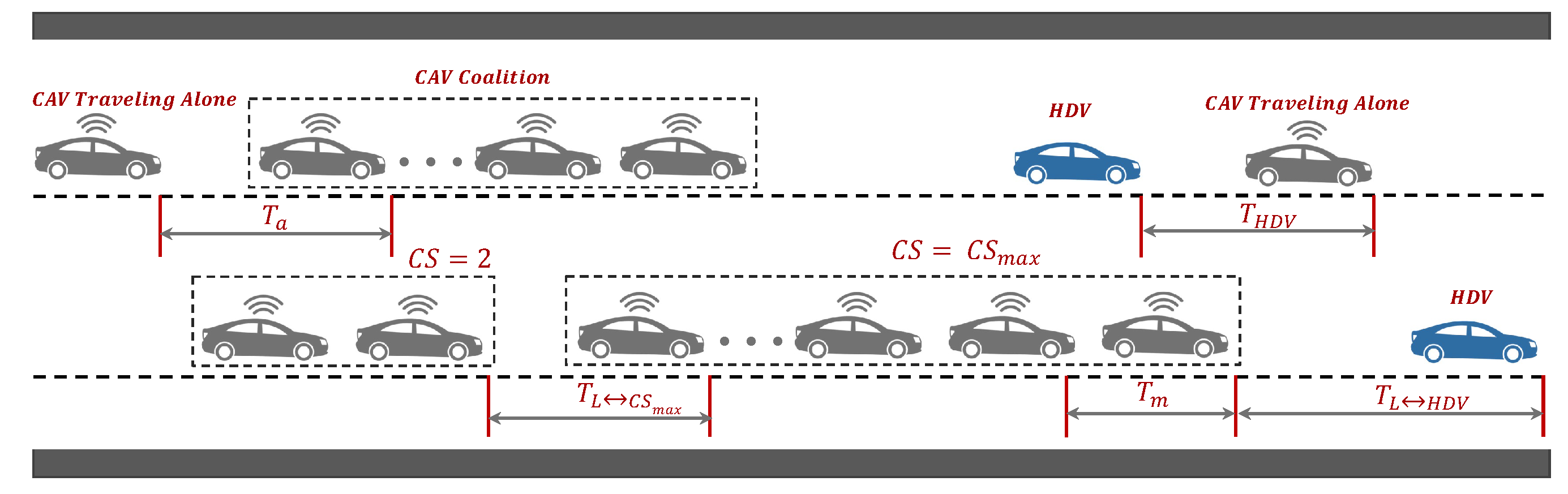
3.1.1. Spatial Arrangement of Vehicles in Mixed Traffic
3.1.2. Coalition Intensity
3.1.3. Probability Distribution of Car-Following Modes
- The spatial probability distribution of an HDV is computed as in Equation (3) where is the market penetration rate of connected autonomous vehicles.
- The probability of the CAV traveling alone and not being a member of any coalition is calculated as in Equation (4) where the represents the intensity of the coalition formation.
- The scenario where the coalition leader follows an HDV requires two conditions to be met at the same time: (i) it must follow a human-driven vehicle, and (ii) it should be traveling in a coalition. The probability distribution can be calculated as in Equation (5).
- The scenario where the coalition leader follows a maximum size coalition should meet two conditions such as it should have a consecutive CAV coalitions ahead of it, as a new coalition is established when the count of CAVs exceeds the , and the vehicle behind it is a CAV. Consequently, the probability of this scenario is computed as follows in Equation (6).
- Assuming that the follower i of a coalition is traveling at a jth position in the coalition where , the probability distribution of this mode is calculated as the sum of the i follower within the coalition, as shown in Equation (8).
3.1.4. Car-following Models for Mixed Traffic Flow
- Intelligent Driver Model—The Intelligent Driver Model (IDM) finds widespread application in the analysis of traffic flow characteristics [23]. With a concise set of parameters that hold clear physical interpretations in line with a driver’s real-world driving familiarity, this model effectively captures the car-following behavior of HDVs. Therefore, this research leverages the IDM to model the behavior of HDVs as shown in Equations (9) and (10).where is the instantaneous acceleration of the vehicle n at time t; and represents the desired maximum acceleration and comfortable deceleration, respectively, represents the velocity of vehicle n during the time t.; denotes the free-flow speed; represents the minimal stopping distance; is the desired spacing; denotes the real gap between vehicle n and the vehicle in front, which is ; is the vehicle length; and is the desired headway.
- Cooperative Adaptive Cruise Control—When connected and autonomous vehicles travel in collaborative convoys, the vehicles engage in cooperative adaptive cruise control mode, facilitated by V2V communication capabilities which allows the vehicles to travel with shorter spacings between the adjacent vehicles. The CACC model [24] is utilized to depict the car-following behaviors of CAVs within the convoys. The formulae of this method are discussed in Equations (10) and (12).where represents the time interval; and denote the control gains; represents the deviation in spacing between the actual and intended spacings of vehicle n at time t; denotes the targeted following distance between the CACC-equipped vehicles.
- Adaptive Cruise Control—The adaptive cruise control (ACC) model [25] developed by the PATH’s laboratory is employed to simulate the car-following behaviors of both individual CAVs traveling alone and the leading CAVs in convoy formations. The mathematical formula to model the ACC is presented in Equation (13).here, represents the control gain related to the spacing error between vehicles; is the control gain associated with speed differences; signifies the desired time headway for individual CAVs; is the headway between the coalition leader following the HDVs, and is the headway between the coalition leader following the maximum size coalition.
3.1.5. The Fundamental Diagram Model—Mixed Traffic Flow
3.2. Pollutant Emission Modeling
- ln: is the natural logarithm function of a real number.
- : represents the rate of instantaneous fuel consumption or emission measured in liter per kilometer (L/km) or grams per second (g/s), respectively.
- e: it represents an indicator for the type of fuel consumption or emissions such as CO2 and NOx emissions. It is important to note that e is not an exponential function.
- : is the instantaneous speed of the CAV in km/h.
- a: is the instantaneous acceleration of the CAV measured in km/h/s.
- : represents the regression coefficient in the model for at speed exponent i and acceleration exponent j for positive accelerations.
- : represents the regression coefficient in the model for at speed exponent i and acceleration exponent j for negative accelerations.
4. Collaborative Convoy Driving—A Coalitional Game
4.1. System Modelling
- Players: it refers to the vehicles operating within the urban settings that strive to achieve their specific goals, such as reducing the consumption of fuel consumption, minimizing traveling time, and obtaining other discounts.
- Coalition: is referred to as a collection of vehicles that create convoys. It is defined as vehicles moving closely together in a synchronized fashion.
- Characteristic Function: it is the function represented as which assigns a value to every coalition. In the context of collaborative driving, encapsulates the benefits and compromises associated with coordination in addition to the restrictions placed on the vehicles. The function acts as a utility function, with every player or coalition striving to optimize its value. A thorough discussion on the modeling of the suggested utility function is available in Section 4.3. When considering a coalition , the utility is determined by aggregating the individual utilities of all vehicles of that coalition. The formation of coalitions provides vehicles with the advantages of fuel savings, reduced travel times, and additional discounts on car insurance, traffic fines, and tolls. Vehicles may come across multiple coalitions, and each vehicle chooses the optimal coalition by maximizing its utility. Given the dynamic environment members of the coalition, represented as , have the liberty to exit the coalition whenever they choose while following the established rules and regulations. Nevertheless, vehicles typically remain within their current coalitions until a more favorable option emerges or until their routes align.
4.2. Underlying Assumptions
- The size of the coalition should be greater than 2 and less or equal to the maximum size of the coalition .
- The utility of a player is exclusively determined by the members of the indicating that external factors have no impact on it.
- The suggested algorithm runs across all vehicles, helping them in determining whether to participate in the coalition.
4.3. Proposed Utility Function for Autonomous Vehicle Coalitions
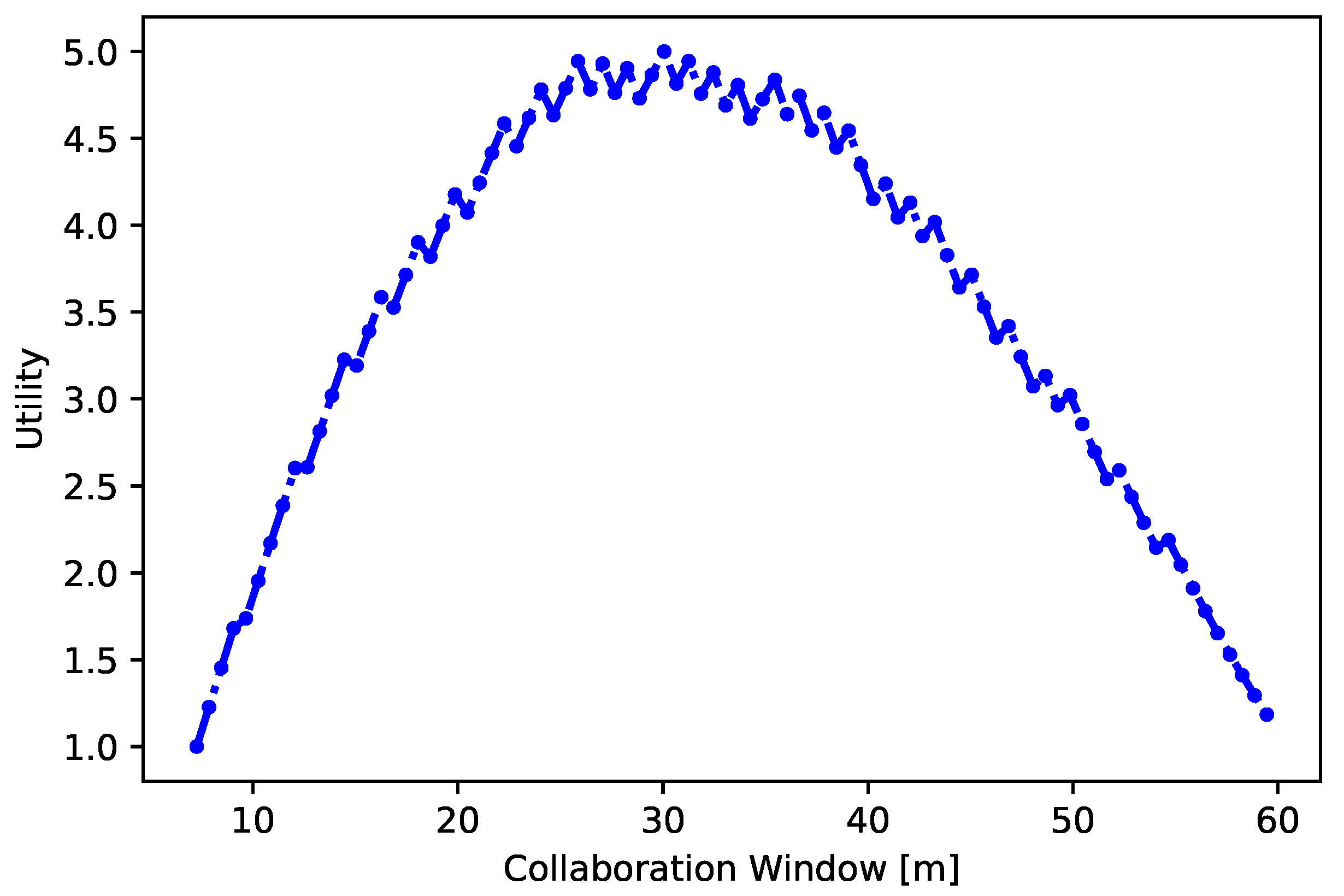
4.3.1. Collaboration Window Function
- Environmental Complexity— The complexity of the environment for vehicle refers to the degree of the dynamicity of its driving environment. This encompasses variables like traffic patterns, weather conditions, pedestrians and cyclists, the presence of other vehicles, and infrastructure components like traffic signals and signs. The environment in which travels, especially at intersections, junctions, and other high-traffic zones, plays a pivotal role in the vehicle’s decision of whether to form and travel in a coalition . Such road segments frequently demand precise coordination and communication among multiple vehicles to ensure secure and efficient navigation. As a result, should be capable of assessing the within its immediate vicinity to make an optimal decision regarding coalition formation.The traffic environment encompasses various external factors that affect autonomous driving such as weather conditions, road conditions, and the behavior of other road participants. We assert that the is an objective characteristic that mainly depends on the physical attributes of the environmental elements such as the static element complexity and the dynamic element complexity . The comprises stationary elements of the environment, such as road segments, tunnels, signage, road markings, vegetation, etc., whereas the encompasses dynamic elements such as vulnerable road users, vehicles, and non-motorized vehicles.To calculate the for , we adopt the equation from the study conducted by Cheng et al. [27]. This equation combines the complexity of both static and dynamic elements, and the result gives the overall complexity of the traffic environment. The formula is presented in Equation (28), where the values of the weighing coefficients and have been set to 0.35 and 0.65, respectively.
- Expected Time to Reach Destination— The expected time for a vehicle to arrive at its destination d in time t represents the time it will take for to journey from its present location to the designated destination. This estimation takes into account various factors, including distance, speed, and potential stops or delays during the journey. The travel time for to arrive at its d when traveling independently is calculated as below:In Equation (30), D represents the distance that must traverse to reach the destination d, with a traveling speed denoted as . represents the count for potential stops that could encounter on its journey to d because of congestion, and represents the duration of time spent at each stop. Calculating plays a pivotal role for CAV in determining whether to establish a coalition. For instance, if calculates its and concludes that it will arrive at its destination d in a relatively brief timeframe, it may not perceive it as beneficial to become part of a coalition . This is due to the fact that the potential time savings achieved by forming may not be sufficient to compensate for the increased expenses associated with collaborating with and modifying the route of a vehicle. Under these scenarios, the vehicle might choose to proceed on its own, resulting in saving time. Therefore, the computation of empowers the vehicle to make well-informed choices regarding coalition formation by weighing the benefits against the associated costs.
- Overlapping Distance—The overlapping route pertains to a specific route of length , which both the vehicle and the coalition can simultaneously travel in the same direction . To ensure safe and efficient travel within the coalition , all vehicles must be synchronized and adhere to this shared route. Therefore, to calculate the , the utilizes various sensor devices to gather and communicate essential data. This information includes speed of the vehicle, position , and the planned traveling route with neighboring vehicles or with the coalition if it is already formed. The traveling route of is compared and synchronized with the route of the coalition , and their similarities are used to determine the of the road segment where their routes overlap.In complex urban settings, the overlapping distance may only span a short distance before vehicles diverge onto separate routes. However, in the controlled highway scenarios, the encompass a substantial segment of the route, influenced by factors such as , etc.
- Speed Difference—The computation of the speed variation between the vehicle and the coalition is calculated using Equation (31). This equation assesses the variance between the desired travel speed V for vehicle on the road and the current V maintained by the vehicles in the coalition .In Equation (31), denotes the speed that vehicle aims to achieve; denotes the speed provided by the to ; and are the minimum and maximum speed limits for , respectively. It is important to note that, a lower value of is considered more favorable for . For instance, if the of exceeds the offered speed (e.g., = 45 km/h and = 35 km/h), might not find it appealing to join the coalition due to the lower offered speed. Conversely, if is lower than (e.g., = 30 km/h and = 45 km/h), it may become more attractive for to be part of the coalition, as it allows for quicker arrival at the destination. However, it is also worth mentioning that while speed is a key factor, other considerations, such as fuel efficiency and maintaining safe and optimal driving conditions, should also be taken into account by when deciding whether to join the coalition.
4.3.2. Objective Function
- Car Insurance Discount— Car insurance discounts serve as a powerful incentive mechanism for vehicles, motivating them to travel in coalition. To encourage this behavior, authorities can call upon insurance companies to offer discounts to collaborating vehicles, provided they adhere to specific criteria, such as the minimum distance, accident history, and coalition size. We believe that this initiative can yield numerous benefits, benefiting both individual vehicles and the environment as a whole.We model this function by defining a base discount rate that is assigned to a vehicle under the given criteria and conditions. Vehicles have to travel a minimum distance in kilometers in the coalition to be eligible for the car insurance discount. This requirement ensures that platooning remains safe and effective. The next step in determining the is to compute the additional distance traveled beyond the required distance, expressed as:In Equation (33) the function calculates the difference between the total distance traveled in the coalition and the that should be traveled in the to benefit from the discount. The additional discount for is then calculated based on the additional distance traveled and a discount rate per distance interval.In Equation (34), the additional distance is divided by 5, representing intervals of 5 km, and then multiplied by the discount rate per interval .The second criterion for computing is to evaluate the accident history. In Equation (35), a 0.05 discount is applied if there have been no accidents while traveling in a coalition; otherwise, no additional discount is given. This discount can be represented as follows:Conversely, if a vehicle is involved in an accident while traveling in a coalition, the accident penalty is applied, as expressed in Equation (36).An additional discount, denoted as , is provided based on the third criterion. A discount of 0.02 is applied if the size of the coalition falls within the range . If exceeds , there is a gradual decrease in the discount, as expressed in Equation (37). This component incentivizes vehicles to maintain the coalition size within the optimal range of four to six vehicles.Finally, the total car insurance discount for collaborative vehicles is determined by combining all these factors in Equation (38).
- Traffic Fine Discount— Traffic fine discounts can offer tangible financial benefits to vehicles that choose to drive in coalitions, directly reducing the cost of driving and making convoy driving an economically attractive option.We introduce a traffic fine discount function, serving as an incentivizing mechanism implemented by transportation authorities to encourage vehicles to travel in coalitions. This function promotes convoy driving by offering varying financial incentives to drivers based on their adherence to the time of day, coalition size, and speed restrictions. By providing these discounts, transportation authorities seek to optimize traffic flow, reduce congestion, and enhance road safety throughout the day. Essentially, this represents a proactive strategy to address traffic-related issues, decrease fuel consumption, and improve overall traffic flow by rewarding collaborative driving behavior and fostering a more efficient and harmonious traffic environment. Subsequently, we discuss the formulation of the traffic fine discount function, denoted as .Let be a binary variable that refers to specific periods during the day when traffic congestion is either at its highest (peak time) or lowest (off-peak time), then the base discount rate can be written as:Equation (39) models the , depending on whether the coalition is formed during peak or off-peak times. A higher is assigned to vehicles when they form coalitions during peak times, leading to improved traffic flow and reduced congestion. Furthermore, to maintain traffic stability, we consider the coalition size, , and introduce a gradual decrease in the discount as increases beyond the maximum coalition size, . Equation (40) reduces the discount rate by 0.02 for each additional vehicle beyond .To adjust the discount based on average coalition speed compared to an acceptable speed range, we employ specific conditional statements. Given the constraints of the urban environment, we maintain the acceptable speed range for coalitions between 50 km/h and 55 km/h. Penalties are applied for speeds beyond this acceptable range, as formulated in Equation (41). Equation (42) combines all the factors to calculate the total .
- Toll Discount—To motivate vehicles to travel in coalitions and incentivize them with toll discounts, authorities can implement a toll discount policy that encourages and rewards collaborative behavior. However, the vehicles have to adhere to specific criteria, such as maintaining the coalition size and the average speed .Let be the total toll discount amount, be the average coalition speed and be the size of the coalition then the can be formulated as:In Equation (43), T represents the base toll amount, while represents the total discount rate. This rate is computed as a combination of the base discount () rate, the discount adjustment factor (), and the speed discount ().The is based on the coalition size, and the maximum discount is granted when falls within the desired acceptable range.The represents an adjustment to the discount rate based on coalition size exceeding . It functions as a penalty for larger coalitions, reducing the discount rate by 0.02 for each additional vehicle beyond , effectively penalizing larger coalitions.The represents the speed-based discount rate. A 0.02 discount is applied when the speed falls within the acceptable range; otherwise, penalties are imposed as the speed exceeds the acceptable range.
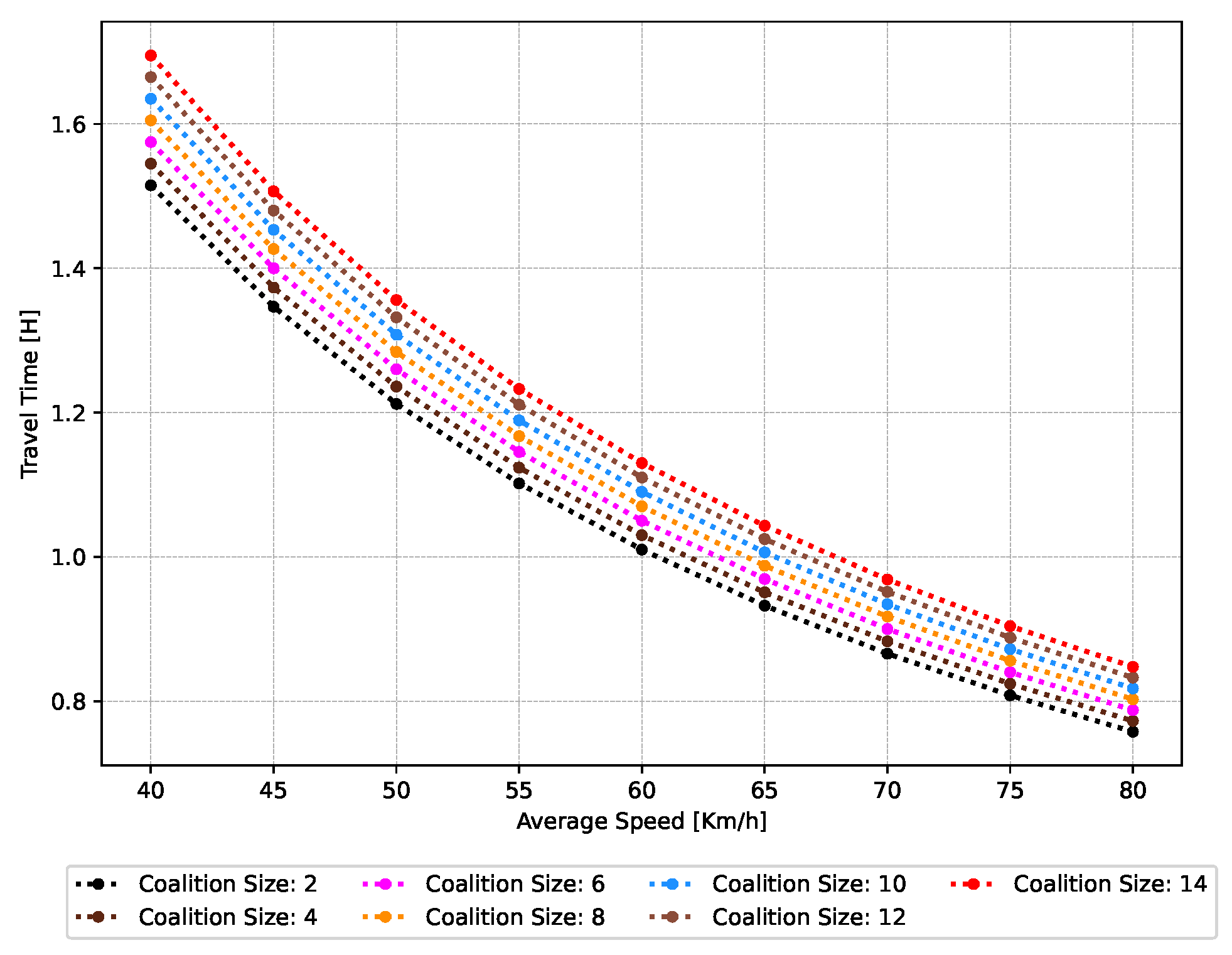
- Travel Time— Traveling within a coalition offers substantial benefits over traveling individually, primarily in terms of significantly reducing the time required to arrive at d. This advantage arises from the tighter inter-vehicle distance within the coalition, which is less than the distance required for vehicles traveling independently along the identical route. By decreasing the spacing among vehicles, the coalition improves traffic flow, leading to reduced travel times. Consequently, vehicles reach their destination d faster compared to if they are traveling individually. The proposed function for estimating the travel time of a vehicle as it travels within a coalition is presented below:In Equation (48), denotes the inter-vehicle spacing between the followers of the coalition ; is the average speed of the vehicles in the ; is the count of stop(s) that the may make on the way to d; and the signifies the duration of time that coalition spends at each stop. The smaller the , the faster reaches its destination d.
- Fuel Consumption— One of the primary incentives to travel in is to achieve significant fuel savings. Traveling in is more fuel-efficient, especially on long journeys. This efficiency stems from a reduction in aerodynamic resistance, a significant contributor to fuel consumption when traveling at high speeds.As a vehicle moves on its own, it disturbs the air in its vicinity, resulting in a pressure disparity extending from the front to the rear. This pressure differential gives rise to an aerodynamic drag force , which acts to impede the vehicle’s onward movement. The magnitude of this drag force grows proportionally to the square of the vehicle’s velocity. Consequently, as the vehicle accelerates, the becomes increasingly pronounced. On the contrary, when vehicles move within the coalition , the front vehicle pierces through the air, creating an area of reduced pressure in its wake. Successive vehicles in coalition travel within this reduced pressure area, which diminishes their . Consequently, vehicles traveling in a require less fuel to sustain their speed compared to when they are traveling individually.Many fuel consumption models have been explored in the literature for estimating fuel consumption, including the ARRB [28], VSP [29], and MEF [30]. In this work, we employ the VT-Micro vehicle-based model to compute the fuel consumption of traveling within based on instantaneous speed V and instantaneous acceleration a. The model is discussed in Equation (25) and the regression coefficients are presented in Appendix A Table A3. Furthermore, the readers are encouraged to look into the authors’ recent publications [31] for the physics-based model, where we simulate the aerodynamic drag component based on varying inter-vehicle spacing and its effect on fuel consumption, which is essential to calculate the fuel consumption of coalition.
4.3.3. Cost Function
- Lane Change Cost— The cost linked to lane changes, symbolized as for vehicle , signifies the expense accrued when switching to another lane, referred to as to become a part of the coalition . This cost is computed by taking into account a range of factors, including the distance traveled to change lanes, the number of lane changes, and the potential collision risk.We design a piecewise function, defined in Equation (50), to calculate the cost. based on two parameters, X and .In Equation (50), the variable X denotes the distance that needs to cover in order to change lanes and merge with ; represents the count of lane changes necessary for vehicle ; the coefficients b and c are utilized in the linear part of the cost function, reflecting the cost associated with lane changes over a certain distance and the symbol stands for the coefficient in the quadratic part of the cost function, denoting the cost associated with lane changes over a squared distance. Incorporating the lane-changing cost into the comprehensive cost function enables vehicles to make more educated choices when determining whether to become part of coalition taking into account the associated risks and expenses associated with changing lanes.
- Catch-up Cost— The vehicles are spatially scattered on the road network. The cost to catch up with the coalition denoted as represents the time that the vehicle takes to join , and it is intricately linked to the speed and the longitudinal gap between the vehicle and the target coalition . The proximity between the two plays a pivotal role in determining the feasibility of the merging process. The is modelled as presented in Equations (51) and (52) below:Firstly, in Equation (51) the longitudinal gap is calculated by taking the difference between the position of denoted as and the denoted as . Equation (52) calculates the by dividing the to the relative speed where the . A shorter distance to the target leads to a lower cost of time, as it reduces the time required for to position itself within the coalition’s formation. Conversely, a greater distance may result in increased time and fuel spent to synchronize the vehicle’s speed and trajectory with that of , emphasizing the critical interplay between distance and the associated cost of time in the context of coalition formation.
- Speed Synchronization Cost— This represents the cost experienced by a vehicle when becoming a part of the coalition necessitating synchronization of its speed with . Specifically, if the coalition is moving at a faster speed V than the vehicle attempting to join, the vehicle might need to accelerate to match the speed of in order to become part of the coalition. This adjustment results in elevated fuel consumption and heightened risk for vehicle , consequently incurring a cost for the vehicle. Consequently, it is important to quantify the speed synchronization cost based on the speed disparity between the vehicle and the coalition.In Equation (53), the denotes the current speed of the , is the current speed of the coalition . The value of is set to zero when vehicle is already a part of coalition . This cost element considers practical factors, such as the need for changes in speed to become a part of , and its magnitude relies on several factors, including the speed disparity between the current speed of the coalition and the current speed of the vehicle . Through experimentation, we observe that constant values within the range of 0.05 to 0.1 are suitable for the parameter .
5. Evaluating the Collaborative Driving Game with Shapley Allocation Analysis
6. Numerical Experiments and Evaluation
6.1. Societal Benefits of Convoy Driving
6.1.1. Traffic Flow
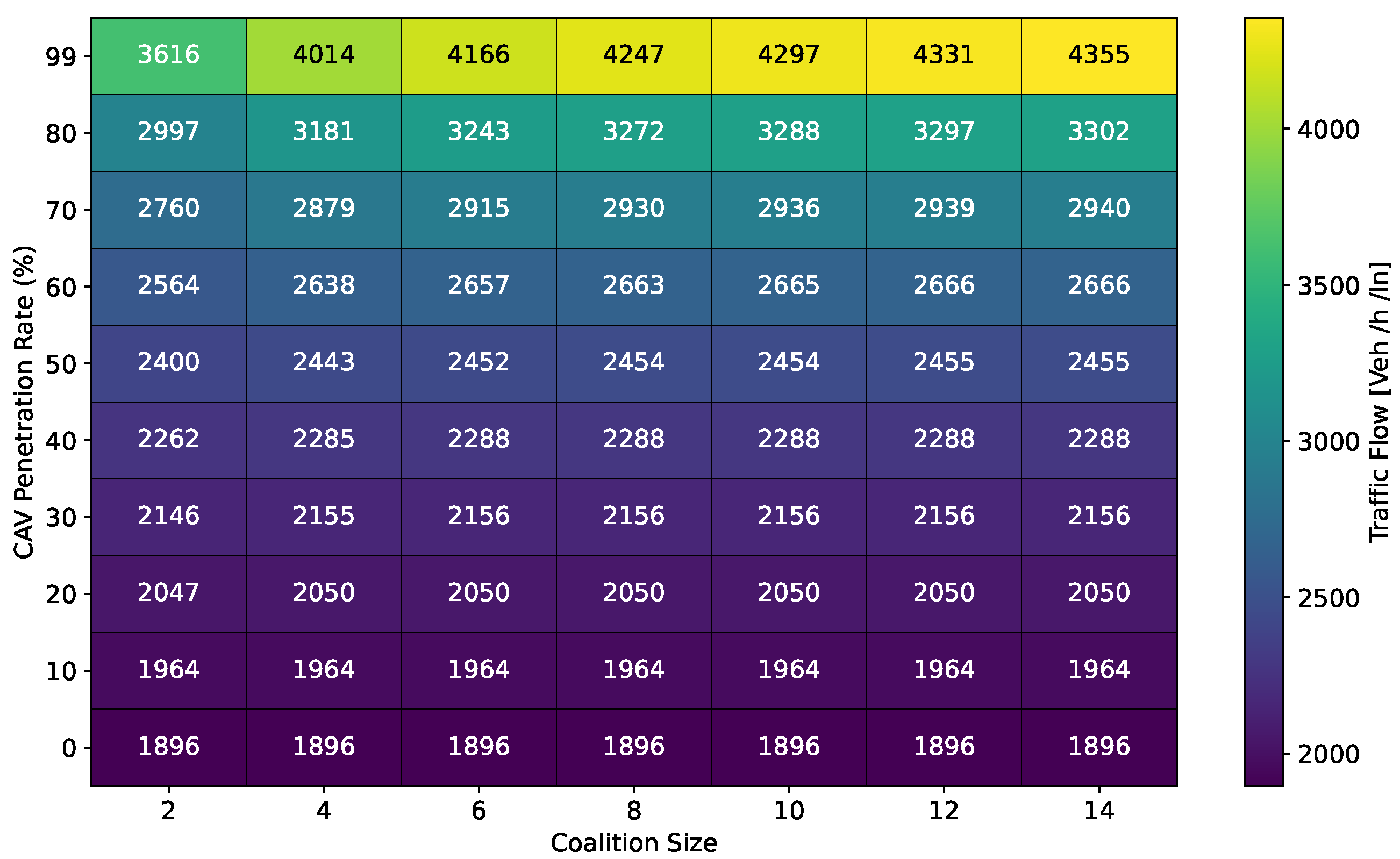
- Optimal Coalition Size—In this experiment, we aim to find the optimal size of a coalition in an urban environment considering different crucial parameters. When the intensity of forming a CAV coalition is low, coalitions are less likely to reach their maximum size. Conversely, when coalition intensity is relatively high, most coalition can attain their maximum size. To investigate the impact of coalition size ranging from (2–14) vehicles on traffic flow considering varying , we set the coalition intensity = 1.0 and incrementally increase CAV penetration from 0% to 99% with a step size of 10.The experimental results presented as a heatmap in Figure 4 reveal that the highest traffic flow measured in vehicles per hour per lane (veh/h/ln) is achieved when both coalition sizes and CAV are relatively high. Increasing coalition size exhibits a gradual improvement in traffic flow capacity. The larger the coalition size, the higher the traffic flow. The heatmap also illustrates that higher correlates with improved capacity, as indicated by the darker colors in the upper section of the map indicating that an increasing number of CAVs positively impacts the traffic flow. However, an intriguing observation is the diminishing returns associated with increasing coalition size beyond a certain threshold. While a larger coalition initially enhances traffic flow capacity, there comes a point where further increasing the coalition size beyond six has a marginal impact on traffic flow, and increasing the CAV penetration rate becomes imperative to increase traffic volume. Therefore, based on these findings, we conclude that the optimal coalition size, while considering the limitations of the urban environment and maintaining traffic flow stability, is 4–6, and we use this as the maximum coalition size in all the subsequent experiments.
- Free Flow Speed— Free-flow speed refers to the maximum speed at which vehicles can travel when there is no congestion or hindrance. In this experiment, we investigate the impact of varying free-flow speeds of coalition ranging from 40 km/h to 80 km/h with an increment of 5 km/h, on traffic flow and traffic density.The result presented in Figure 5 shows the optimal traffic flow and density for each . It demonstrates a strong positive correlation between and traffic flow. As the increases, the capacity of the roadway to accommodate vehicles also rises. This relationship is intuitive, as higher speeds allow vehicles to cover more ground in a given time, resulting in an increased flow of vehicles. Conversely, the relationship between and traffic density is inversely proportional. As increases, traffic density measured in vehicle per kilometer per lane (veh/km/ln) decreases. Higher encourage vehicles to maintain greater spacing between each other, reducing the potential for traffic congestion.Higher can alleviate congestion, reduce travel times, and enhance overall road network efficiency; however, lower traffic densities contribute to improved road safety and reduced pollutant emissions. Therefore, we conclude that, in a complex urban scenario, a free-flow speed of 55 km/h represents an optimal balance. It maximizes traffic flow while maintaining safe and manageable traffic densities.
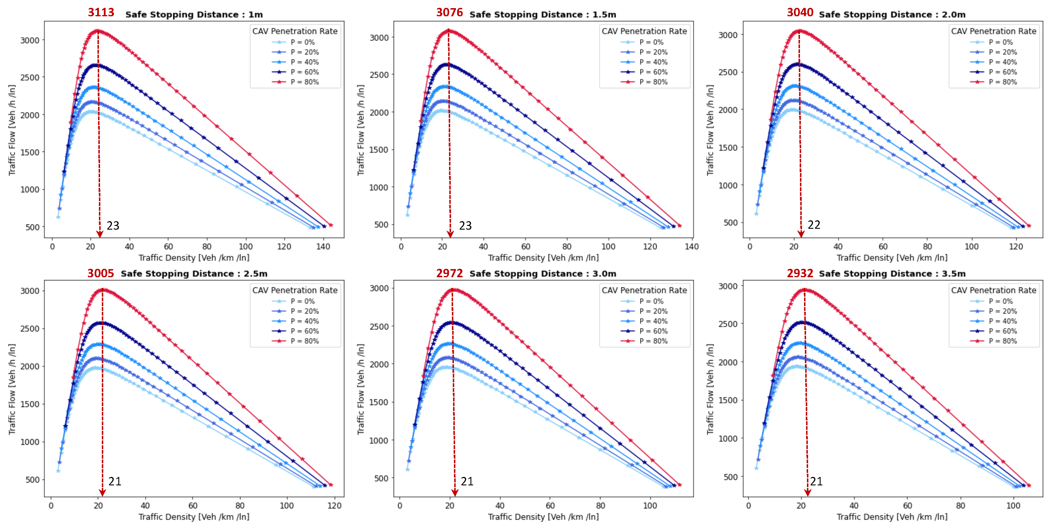
- Safe Stopping Distance— In this experiment, we investigate the impact of varying safe stopping distances from 1 m to 3.5 m with an increment of 0.5 m on both traffic flow and traffic density under various CAV and the . In Figure 6, the x-axis represents traffic density in (veh/km/ln), while the y-axis depicts traffic flow in (veh/h/ln) and the results are showcased for different CAV ranging from 0% to 80%.The results show that increasing the between the coalition members tends to decrease traffic flow. A larger means that vehicles need more inter-vehicle distance to stop safely, resulting in fewer vehicles passing a particular point on the road within a given time frame, leading to a reduction in traffic flow. As the increases, traffic density, representing the number of vehicles per unit length of the road, tends to decrease. This decrease in traffic density is a direct outcome of the increase in inter-vehicle distance, with more significant safety margins causing vehicles to spread out, thereby reducing congestion. The findings of this research show that selecting the optimal safe stopping distance should strike a balance between safety, traffic efficiency, road conditions, and the level of automation in the vehicles on the road. Therefore, we conclude that a safe stopping distance of 2 m is optimal, achieving a balance between safety and traffic efficiency.
- Impact of Coalition Intensity and CAV penetration rate on Traffic Flow-Density Relationship— To investigate how the CAV impacts the fundamental diagram of mixed traffic flow, the coalition intensity () is set to = [0, 0.25, 0.5, 0.75, 1]. For each value of , the maximum penetration rate is computed using Equation (2). The experimental results, presented in Figure 7, illustrate the relationship between traffic flow and traffic density under various conditions of and . Additionally, for each value of , the maximum flow and the critical density are annotated on the graph.The term free flow regime in the graphs refers to a traffic state where the coalitions move smoothly and efficiently at or near their desired speeds. In contrast, the congested flow regime represents a traffic state characterized by high traffic density and reduced vehicle speeds. It is evident from Figure 7 that as the coalition intensity ranging from 0 to 1 increases, traffic flow generally improves across all levels of CAV penetration. However, the extent of traffic capacity growth varies at different coalition intensities, with a more pronounced impact observed when coalition intensity is ( = 0.75 or 1.0). Higher coalition intensity results in a more organized and efficient traffic flow, reducing congestion and increasing the number of vehicles passing through a lane per hour. Furthermore, irrespective of coalition intensity, an increase in CAV penetration rate typically leads to improved traffic flow. The results also show that the maximum traffic flow of 4339 (veh/h/ln) at = 1.0 = 99% increases the traffic flow by 88.81% compared to the maximum traffic flow of 2296 (veh/h/ln) at = 0 and = 50%. The findings of this experiment suggest that achieving high traffic flow rates and reducing congestion necessitates a combination of both high coalition intensity and a high CAV penetration rate.
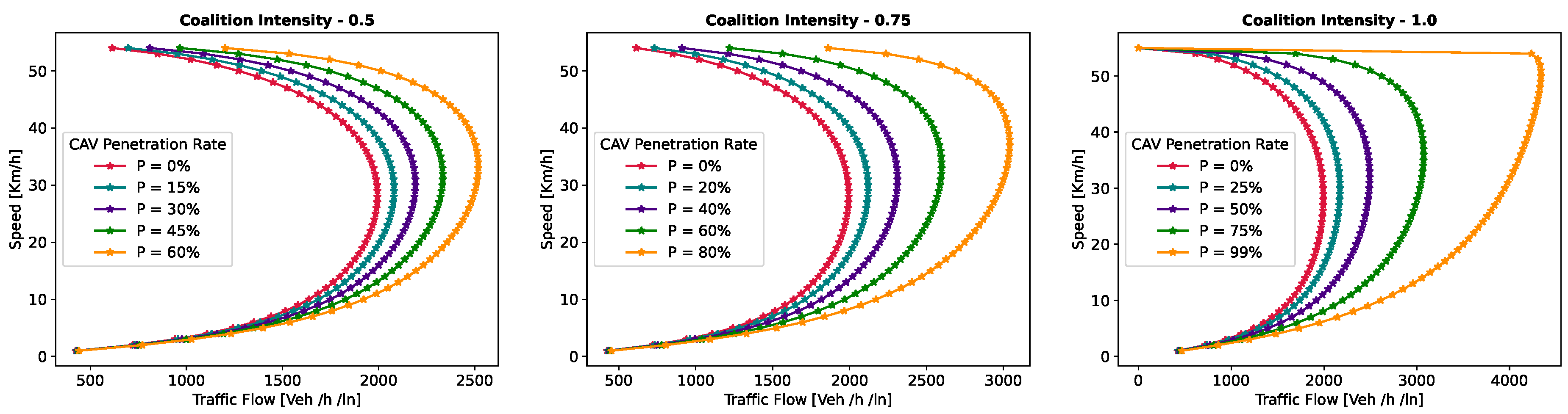
- Speed-Density Relationship— In this experiment, we investigate the speed–density relationships for high levels of coalition intensity, = [0.5, 0.75, and 1.0], and various levels of CAV penetration rates, ranging from 0% to 99%. The results presented in Figure 8 indicate that at low traffic densities, traffic typically moves at or near the free flow speed, which is the speed at which vehicles travel without congestion. However, as traffic density increases, congestion begins to impact traffic speed, resulting in a decrease in speed. Higher CAV have a notable positive effect on traffic flow and speed, especially at moderate to high traffic densities. CAVs play a crucial role in mitigating congestion and maintaining relatively higher speeds compared to non-CAV scenarios. This impact of CAV penetration on traffic speed is more pronounced at higher coalition intensity levels where CAVs significantly influence traffic flow and higher speeds. Therefore, we conclude that CAV coalitions have the potential to enhance traffic conditions by reducing congestion and maintaining higher speeds, especially in scenarios with greater platoon intensity.
- Speed-Flow Relationship— In this experiment, we investigate the speed–flow relationship for different coalition intensities (0.5, 0.75, and 1.0) under varying levels of CAV penetration rates, shedding light on how traffic speed changes with the flow of traffic on a roadway. The result presented in Figure 9 shows that the presence of CAVs has a significantly positive impact on traffic flow. Higher CAV penetration rates lead to more favorable speed–flow curves. As CAVs become more prevalent, traffic flow remains efficient, and vehicles can maintain higher speeds even as traffic density increases. However, this effect is most pronounced at higher coalition intensities, where CAVs play a pivotal role in achieving near-optimal traffic conditions and significant improvements in traffic flow and speed stability.
6.1.2. Pollutant Emission
- Carbon Dioxide Emission— To evaluate the impact of coalition-driven travel on CO2 emission, the penetration rate of CAV is set to . The instantaneous speed and acceleration at each time step are derived based on the simulation results. The experimental findings presented in Figure 10, depict that there is a clear correlation between speed and CO2 emissions. Lower speeds exhibit notably lower emissions, while higher speeds are associated with slightly increased emissions.At lower speeds, ranging from 40 to 55 km/h, the results show a noticeable decline in CO2 as the coalition size increases. This suggests that when vehicles travel at lower speeds and maintain a shorter following distance, reduced air resistance from drafting behind the lead vehicle improves fuel efficiency, resulting in lower CO2 emissions. Although the emissions exhibit slight fluctuations, it shows that forming larger coalitions at lower speeds consistently reduces CO2 emissions per vehicle. Furthermore, the reduction in CO2 is more significant when transitioning from a small coalition to a moderate-sized one, with the additional reduction becoming less pronounced as the coalition size further increases.In contrast, at higher speeds between 60 and 80 km/h, as the coalition size increases, CO2 tends to stabilize and show a mild increase. This phenomenon can be attributed to the diminished aerodynamic advantages of drafting at increased velocities. At these speeds, the advantages of reduced air resistance are outweighed by other factors such as increased engine load and fuel consumption. Consequently, CO2 per unit of time remains relatively constant and slightly rises with coalition size.The findings highlight the complex interplay between speed, coalition size, and emissions and demonstrate that convoy driving at both lower and higher speeds can lead to substantial reductions in CO2; however, the rate of reduction diminishes as the coalition size increases, suggesting that there is an optimal coalition size that maximizes the advantages of collaborative driving in terms of CO2 reduction. These results can assist policymakers in setting speed limits and promoting coalition-based transportation to reduce CO2 emissions.
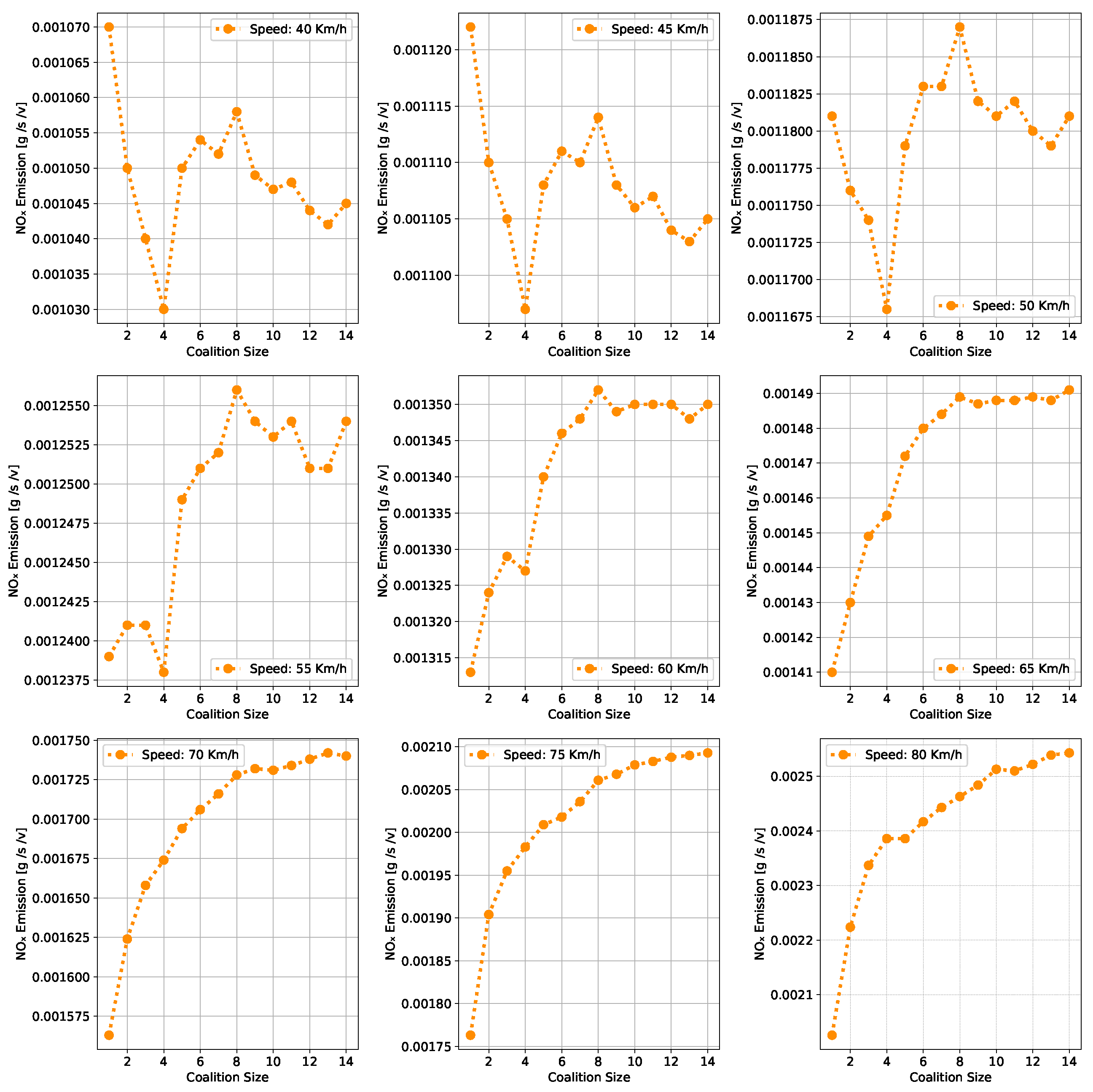
- Nitrogen Oxide Emission— To assess how traveling in coalition affects the NOx emission, the penetration rate of CAVs is set to . The instantaneous speed and acceleration at each time step are collected using the CACC model. Observing the results presented in Figure 11 shows several trends emerge. Firstly, there is a noticeable general increase in NOx as coalition size grows, regardless of speed. This suggests that as more vehicles join the coalition, the overall emissions tend to rise. However, the rate of increase varies with speed, with higher speeds typically resulting in steeper NOx increases with coalition size.At lower speeds, from 40 to 50 km/h, a relatively consistent pattern of NOx is observed. Emissions consistently remain low, hovering around 0.00103 to 0.00118 g/s/v across various coalition sizes. This suggests that forming coalitions at lower speeds has a minimal impact on NOx as the differences between coalition sizes are marginal.Conversely, at higher speeds ranging from 55 to 80 km/h, the NOx exhibits a more noticeable upward trend as the coalition size increases. Emissions gradually increase from approximately 0.00122 g/s/v at a coalition size of 1 to around 0.0024 g/s/v at a coalition size of 14. This indicates that coalition at higher speeds leads to higher NOx likely due to increased engine load and the need for more frequent acceleration, which can occur in larger coalitions.The findings highlight that there is a certain balance to be struck between speed and coalition size for minimizing NOx emissions as the relationship between these variables is not consistent across all speed ranges. Such insights are crucial for policymakers to make informed decisions regarding the implementation of platooning strategies aimed at achieving both efficiency and environmental sustainability in transportation systems.
6.2. Benefits of Coalition-Driven at Individual Vehicle Level
6.2.1. Aggregated Utility of Traveling in Coalition
6.2.2. Discount on Car Insurance
6.2.3. Discount on Traffic Fine
6.2.4. Discount on Toll
6.2.5. Time-Saving Benefits of Coalition Travel
6.2.6. Fuel Consumption Benefits in Coalition Travel
7. Conclusions
- When the intensity of forming a coalition is low, coalitions are less likely to reach their maximum size, and vice versa. The optimal coalition size is found to be 4–6 vehicles, which maintains the stability and safety of the urban environment. However, the coalition size has little effect on the flow when it exceeds 6.
- A higher free-flow speed has a positive impact on the maximum traffic flow in mixed-traffic settings. As free-flow speed gradually rises, the maximum traffic volume for mixed traffic also gradually increases, although the ideal traffic density decreases over time. The recommended optimal free-flow coalition speed is 55 km/h.
- The maximum traffic flow of mixed traffic is adversely affected by the safe stopping distance. As the minimum safe distance gradually increases, both the maximum traffic volume and the ideal traffic density for mixed traffic gradually decrease. The experiments show that 2 m is recommended to achieve a balance between safety and traffic efficiency.
- As the coalition intensity increases, traffic flow generally improves across all levels of CAV penetration. However, the extent of traffic capacity growth varies at different platoon intensities, with a more pronounced impact observed when coalition intensity is = 0.75 and 1.0.
- At low penetration rates, the intensity of connected and autonomous vehicle coalitions has a minor influence on the attributes of mixed traffic flow.
- The levels of CO2, NOx, and fuel consumption increase with higher speeds and larger coalition sizes.
Author Contributions
Funding
Institutional Review Board Statement
Informed Consent Statement
Data Availability Statement
Conflicts of Interest
Abbreviations
| Notation | Description |
| Connected and autonomous vehicle | |
| Coalition of CAVs | |
| Instantaneous acceleration of the vehicle | |
| Free-flow speed of the vehicles | |
| Equilibrium speed | |
| Average speed of vehicles in | |
| Speed of vehicle n at time t | |
| Inter-vehicle spacing in the coalition | |
| Penetration rate of CAVs | |
| Penetration rate of CAVs | |
| Intensity of forming a coalition | |
| Average headway among vehicles in mixed traffic flow | |
| Traffic Density | |
| Coalition size | |
| Maximum coalition size | |
| Traffic volume | |
| Pollutant emission | |
| Carbon dioxide | |
| Nitrogen Oxides | |
| Neighbouring Vehicles | |
| Collaboration Window | |
| Complexity of the environment | |
| Overlapping distance between the CAV and the coalition | |
| Cost of joining a coalition | |
| Complexity of static elements in the environment | |
| Complexity of static elements in the environment | |
| Length of the vehicle | |
| Length of the route | |
| Desired speed of CAV | |
| Longitudinal gap between the CAV and the coalition | |
| Relative speed | |
| Current speed of the coalition | |
| Current speed of the vehicle | |
| Shapley value of player i |
Appendix A

| For | For | ||||||||
|---|---|---|---|---|---|---|---|---|---|
| 6.916 | 0.217 | 2.35 | −3.64 | 6.915 | −0.032 | −9.17 | −2.89 | ||
| 0.02754 | 9.68 | −1.75 | 8.35 | 0.0284 | 8.53 | 1.15 | −3.06 | ||
| −2.07 | −1.01 | 1.97 | −1.02 | −2.27 | −6.59 | −1.29 | −2.68 | ||
| 9.80 | 3.66 | −1.08 | 8.50 | 1.11 | 3.20 | 7.56 | 2.95 | ||
| For | For | ||||||||
|---|---|---|---|---|---|---|---|---|---|
| −1.08 | 0.2369 | 1.47 | −7.82 | −1.08 | 0.2085 | 2.19 | 8.82 | ||
| 1.79 | 4.05 | −3.75 | 1.05 | 2.11 | 1.07 | 6.55 | 6.27 | ||
| 2.41 | −4.08 | −1.28 | 1.52 | 1.63 | −3.23 | −9.43 | −1.01 | ||
| −1.06 | 9.42 | 1.86 | 4.42 | −5.83 | 1.83 | 4.47 | 4.57 | ||
| For | For | ||||||||
|---|---|---|---|---|---|---|---|---|---|
| −7.735 | 0.2295 | −5.61 | 9.77 | −7.735 | −0.01799 | −4.27 | 1.88 | ||
| 0.02799 | 0.0068 | −7.72 | 8.38 | 0.02804 | 7.72 | 8.38 | 3.39 | ||
| −2.23 | −4.40 | 7.90 | 8.17 | −2.20 | −5.22 | −7.44 | 2.77 | ||
| 1.09 | 4.80 | 3.27 | −7.79 | 1.08 | 2.47 | 4.87 | 3.79 | ||
References
- Malik, S.; Khan, M.A.; El-Sayed, H. Collaborative autonomous driving—A survey of solution approaches and future challenges. Sensors 2021, 21, 3783. [Google Scholar] [CrossRef] [PubMed]
- Bansal, P.; Kockelman, K.M. Forecasting Americans’ long-term adoption of connected and autonomous vehicle technologies. Transp. Res. Part A Policy Pract. 2017, 95, 49–63. [Google Scholar] [CrossRef]
- Yao, Z.; Jiang, H.; Cheng, Y.; Jiang, Y.; Ran, B. Integrated schedule and trajectory optimization for connected automated vehicles in a conflict zone. IEEE Trans. Intell. Transp. Syst. 2020, 23, 1841–1851. [Google Scholar] [CrossRef]
- Pi, D.; Xue, P.; Wang, W.; Xie, B.; Wang, H.; Wang, X.; Yin, G. Automotive platoon energy-saving: A review. Renew. Sustain. Energy Rev. 2023, 179, 113268. [Google Scholar] [CrossRef]
- Malik, S.; Khan, M.A.; El-Sayed, H.; Khan, J.; Ullah, O. How do autonomous vehicles decide? Sensors 2022, 23, 317. [Google Scholar] [CrossRef] [PubMed]
- Yao, Z.; Gu, Q.; Jiang, Y.; Ran, B. Fundamental diagram and stability of mixed traffic flow considering platoon size and intensity of connected automated vehicles. Phys. A Stat. Mech. Its Appl. 2022, 604, 127857. [Google Scholar] [CrossRef]
- Jiang, Y.; Zhu, F.; Gu, Q.; Wu, Y.; Wen, X.; Yao, Z. Influence of CAVs platoon characteristics on fundamental diagram of mixed traffic flow. Phys. A Stat. Mech. Its Appl. 2023, 624, 128906. [Google Scholar] [CrossRef]
- Yao, Z.; Wu, Y.; Wang, Y.; Zhao, B.; Jiang, Y. Analysis of the impact of maximum platoon size of CAVs on mixed traffic flow: An analytical and simulation method. Transp. Res. Part Emerg. Technol. 2023, 147, 103989. [Google Scholar] [CrossRef]
- Li, R.; Sun, S.; Wu, Y.; Hao, H.; Wen, X.; Yao, Z. Fundamental diagram of mixed traffic flow considering time lags, platooning intensity, and the degradation of connected automated vehicles. Phys. A Stat. Mech. Its Appl. 2023, 627, 129130. [Google Scholar] [CrossRef]
- Ma, K.; Wang, H.; Ruan, T. Analysis of road capacity and pollutant emissions: Impacts of Connected and automated vehicle platoons on traffic flow. Phys. A Stat. Mech. Its Appl. 2021, 583, 126301. [Google Scholar] [CrossRef]
- Jiang, Y.; Zhu, F.; Yao, Z.; Gu, Q.; Ran, B. Platoon Intensity of Connected Automated Vehicles: Definition, Formulas, Examples, and Applications. J. Adv. Transp. 2023, 2023, 3325530. [Google Scholar] [CrossRef]
- Hang, P.; Lv, C.; Huang, C.; Xing, Y.; Hu, Z. Cooperative decision making of connected automated vehicles at multi-lane merging zone: A coalitional game approach. IEEE Trans. Intell. Transp. Syst. 2021, 23, 3829–3841. [Google Scholar] [CrossRef]
- Yang, L.; Zhan, J.; Shang, W.L.; Fang, S.; Wu, G.; Zhao, X.; Deveci, M. Multi-Lane Coordinated Control Strategy of Connected and Automated Vehicles for On-Ramp Merging Area Based on Cooperative Game. IEEE Trans. Intell. Transp. Syst. 2023, 24, 13448–13461. [Google Scholar] [CrossRef]
- Hang, P.; Lv, C.; Huang, C.; Hu, Z. Cooperative decision making of lane-change for automated vehicles considering human-like driving characteristics. In Proceedings of the 2021 40th Chinese Control Conference (CCC), Shanghai, China, 26–28 July 2021; pp. 6106–6111. [Google Scholar]
- Hang, P.; Huang, C.; Hu, Z.; Lv, C. Decision making for connected automated vehicles at urban intersections considering social and individual benefits. IEEE Trans. Intell. Transp. Syst. 2022, 23, 22549–22562. [Google Scholar] [CrossRef]
- Ledbetter, B.; Wehunt, S.; Rahman, M.A.; Manshaei, M.H. LIPs: A protocol for leadership incentives for heterogeneous and dynamic platoons. In Proceedings of the 2019 IEEE 43rd Annual Computer Software and Applications Conference (COMPSAC), Milwaukee, WI, USA, 15–19 July 2019; Volume 1, pp. 535–544. [Google Scholar]
- Chen, C.; Xiao, T.; Qiu, T.; Lv, N.; Pei, Q. Smart-contract-based economical platooning in blockchain-enabled urban internet of vehicles. IEEE Trans. Ind. Inf. 2019, 16, 4122–4133. [Google Scholar] [CrossRef]
- Earnhardt, C.; Groelke, B.; Borek, J.; Pelletier, E.; Brennan, S.; Vermillion, C. Cooperative exchange-based platooning using predicted fuel-optimal operation of heavy-duty vehicles. IEEE Trans. Intell. Transp. Syst. 2022, 23, 17312–17324. [Google Scholar] [CrossRef]
- Jiang, Y.; Sun, S.; Zhu, F.; Wu, Y.; Yao, Z. A mixed capacity analysis and lane management model considering platoon size and intensity of CAVs. Phys. A Stat. Mech. Its Appl. 2023, 615, 128557. [Google Scholar] [CrossRef]
- Jiang, Y.; Ren, T.; Ma, Y.; Wu, Y.; Yao, Z. Traffic safety evaluation of mixed traffic flow considering the maximum platoon size of connected automated vehicles. Phys. A Stat. Mech. Its Appl. 2023, 612, 128452. [Google Scholar] [CrossRef]
- Gong, B.; Wang, F.; Lin, C.; Wu, D. Modeling HDV and CAV mixed traffic flow on a foggy two-lane highway with cellular automata and game theory model. Sustainability 2022, 14, 5899. [Google Scholar] [CrossRef]
- Wang, W.; Wu, B. The fundamental diagram of mixed-traffic flow with CACC vehicles and human-driven vehicles. J. Transp. Eng. Part A Syst. 2023, 149, 04022116. [Google Scholar] [CrossRef]
- Treiber, M.; Hennecke, A.; Helbing, D. Congested traffic states in empirical observations and microscopic simulations. Phys. Rev. E 2000, 62, 1805. [Google Scholar] [CrossRef]
- Milanés, V.; Shladover, S.E.; Spring, J.; Nowakowski, C.; Kawazoe, H.; Nakamura, M. Cooperative adaptive cruise control in real traffic situations. IEEE Trans. Intell. Transp. Syst. 2013, 15, 296–305. [Google Scholar] [CrossRef]
- Bageshwar, V.L.; Garrard, W.L.; Rajamani, R. Model predictive control of transitional maneuvers for adaptive cruise control vehicles. IEEE Trans. Veh. Technol. 2004, 53, 1573–1585. [Google Scholar] [CrossRef]
- Rakha, H.; Ahn, K.; Trani, A. Development of VT-Micro model for estimating hot stabilized light duty vehicle and truck emissions. Transp. Res. Part D Transp. Environ. 2004, 9, 49–74. [Google Scholar] [CrossRef]
- Cheng, Y.; Liu, Z.; Gao, L.; Zhao, Y.; Gao, T. Traffic risk environment impact analysis and complexity assessment of autonomous vehicles based on the potential field method. Int. J. Environ. Res. Public Health 2022, 19, 10337. [Google Scholar] [CrossRef]
- Akcelik, R. Efficiency and drag in the power-based model of fuel consumption. Transp. Res. Part B Methodol. 1989, 23, 376–385. [Google Scholar] [CrossRef]
- Jimenez-Palacios, J.L. Understanding and Quantifying Motor Vehicle Emissions with Vehicle Specific Power and TILDAS Remote Sensing; Massachusetts Institute of Technology: Cambridge, MA, USA, 1998. [Google Scholar]
- Lei, W.; Chen, H.; Lu, L. Microscopic emission and fuel consumption modeling for light-duty vehicles using portable emission measurement system data. World Acad. Sci. Eng. Technol. 2010, 66, 918–925. [Google Scholar]
- Malik, S.; Khan, M.A.; El-Sayed, H.; Khan, M.J. Should Autonomous Vehicles Collaborate in a Complex Urban Environment or Not? Smart Cities 2023, 6, 2447–2483. [Google Scholar] [CrossRef]
- Shapley, L.S.; Shubik, M. A method for evaluating the distribution of power in a committee system. Am. Political Sci. Rev. 1954, 48, 787–792. [Google Scholar] [CrossRef]
- Han, S.; Wang, H.; Su, S.; Shi, Y.; Miao, F. Stable and efficient Shapley value-based reward reallocation for multi-agent reinforcement learning of autonomous vehicles. In Proceedings of the 2022 International Conference on Robotics and Automation (ICRA), Philadelphia, PA, USA, 23–27 May 2022; pp. 8765–8771. [Google Scholar]
- Song, M.; Chen, F.; Ma, X. Organization of autonomous truck platoon considering energy saving and pavement fatigue. Transp. Res. Part D Transp. Environ. 2021, 90, 102667. [Google Scholar] [CrossRef]
- Typaldos, P.; Papamichail, I.; Papageorgiou, M. Minimization of fuel consumption for vehicle trajectories. IEEE Trans. Intell. Transp. Syst. 2020, 21, 1716–1727. [Google Scholar] [CrossRef]


| Ref. | Coalition Intensity | Coalition Size | Penetration Rate | Societal Benefits | Policy Formulation | Individual Benefits | ||||||||||
|---|---|---|---|---|---|---|---|---|---|---|---|---|---|---|---|---|
| Relationships & Characteristics of Fundamental Diagram | Pollutant Emission | |||||||||||||||
| Volume–Density | Speed–Density | Speed–Volume | Impact of Free Flow Speed | CO2 | NOx | Car Insurance Discount | Traffic Fine Discount | Toll Discount | Fuel Consumption | Travel Time | Other | |||||
| [6] | ✓ | ✓ | ✓ | ✓ | ||||||||||||
| [7] | ✓ | ✓ | ✓ | ✓ | ✓ | ✓ | ||||||||||
| [8] | ✓ | ✓ | ✓ | ✓ | ✓ | |||||||||||
| [9] | ✓ | ✓ | ✓ | ✓ | ✓ | ✓ | ||||||||||
| [10] | ✓ | ✓ | ✓ | ✓ | ||||||||||||
| [11] | ✓ | ✓ | ✓ | ✓ | ||||||||||||
| [12] | ✓ | |||||||||||||||
| [13] | ✓ | ✓ | ||||||||||||||
| [14] | ✓ | |||||||||||||||
| [15] | ✓ | |||||||||||||||
| [19] | ✓ | ✓ | ✓ | |||||||||||||
| [20] | ✓ | ✓ | ||||||||||||||
| [21] | ✓ | ✓ | ✓ | |||||||||||||
| [22] | ✓ | ✓ | ✓ | |||||||||||||
| This paper | ✓ | ✓ | ✓ | ✓ | ✓ | ✓ | ✓ | ✓ | ✓ | ✓ | ✓ | ✓ | ✓ | ✓ | ✓ | |
| Headway | Description |
|---|---|
| = | Spacing between human driven vehicles. |
| Spacing between CAVs traveling alone. | |
| Spacing between the CAV leader following an HDV. | |
| Spacing between the CAV leader following a CAV coalition. | |
| Spacing between coalition followers. |
| Parameter | Unit | Value | Description |
|---|---|---|---|
| Km/h | 45 | Current speed of the vehicle | |
| Km/h | 50 | Desired speed of the vehicle | |
| Km/h | 55 | Current speed of the coalition | |
| Km/h | 40–80 | Coalition speed | |
| , | - | 0.35, 0.65 | Weighing coefficients of |
| m | 5 | Length of the vehicle | |
| 6 | Size of the coalition | ||
| m | 2 | Safe stopping distance | |
| s | 1.5 | Spacing between HDVs | |
| s | 1.1 | Spacing between CAVs traveling alone | |
| s | 1.1 | Spacing between leader of coalition and preceding HDV | |
| s | 1.0 | Spacing between leader following a maximum-coalition | |
| s | 0.6 | Spacing between the coalition followers | |
| 0.9 | Complexity of the environment | ||
| 0.1 | Coordination parameter | ||
| 0.6 | coefficient | ||
| 6 | Number of vehicles in the coalition | ||
| Km/h | 55 | Free flow speed | |
| % | 0–100 | CAV Penetration rate | |
| 0–1 | CAV Coalition Intensity | ||
| 2–14 | Coalition size range | ||
| 6 | Maximum coalition size | ||
| Km | 100 | Minimum distance | |
| Km/h | 55, 65, 75 | Coalition Average Speed |
| 3.0 | 3.5 | 3.48 | 4.0 | 4.3 | 4.85 |
Disclaimer/Publisher’s Note: The statements, opinions and data contained in all publications are solely those of the individual author(s) and contributor(s) and not of MDPI and/or the editor(s). MDPI and/or the editor(s) disclaim responsibility for any injury to people or property resulting from any ideas, methods, instructions or products referred to in the content. |
© 2023 by the authors. Licensee MDPI, Basel, Switzerland. This article is an open access article distributed under the terms and conditions of the Creative Commons Attribution (CC BY) license (https://creativecommons.org/licenses/by/4.0/).
Share and Cite
Malik, S.; Khan, M.A.; El-Sayed, H.; Khan, M.J. Unlocking Mutual Gains—An Experimental Study on Collaborative Autonomous Driving in Urban Environment. Sensors 2024, 24, 182. https://doi.org/10.3390/s24010182
Malik S, Khan MA, El-Sayed H, Khan MJ. Unlocking Mutual Gains—An Experimental Study on Collaborative Autonomous Driving in Urban Environment. Sensors. 2024; 24(1):182. https://doi.org/10.3390/s24010182
Chicago/Turabian StyleMalik, Sumbal, Manzoor Ahmed Khan, Hesham El-Sayed, and Muhammad Jalal Khan. 2024. "Unlocking Mutual Gains—An Experimental Study on Collaborative Autonomous Driving in Urban Environment" Sensors 24, no. 1: 182. https://doi.org/10.3390/s24010182
APA StyleMalik, S., Khan, M. A., El-Sayed, H., & Khan, M. J. (2024). Unlocking Mutual Gains—An Experimental Study on Collaborative Autonomous Driving in Urban Environment. Sensors, 24(1), 182. https://doi.org/10.3390/s24010182