

Tool Health Monitoring of a Milling Process Using Acoustic Emissions and a ResNet Deep Learning Model


 , , ,
, , ,
Abstract
1. Introduction
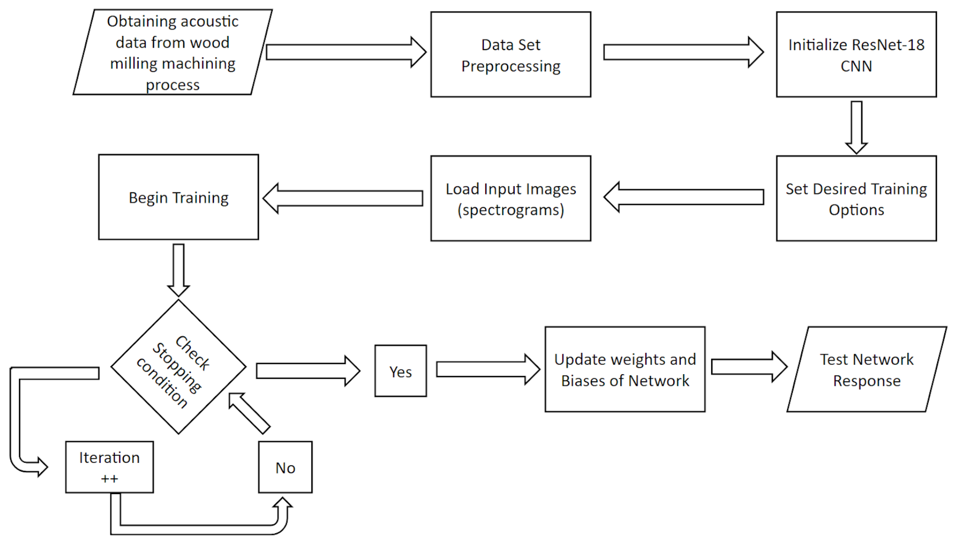
2. Proposed Technique
3. Materials and Methods
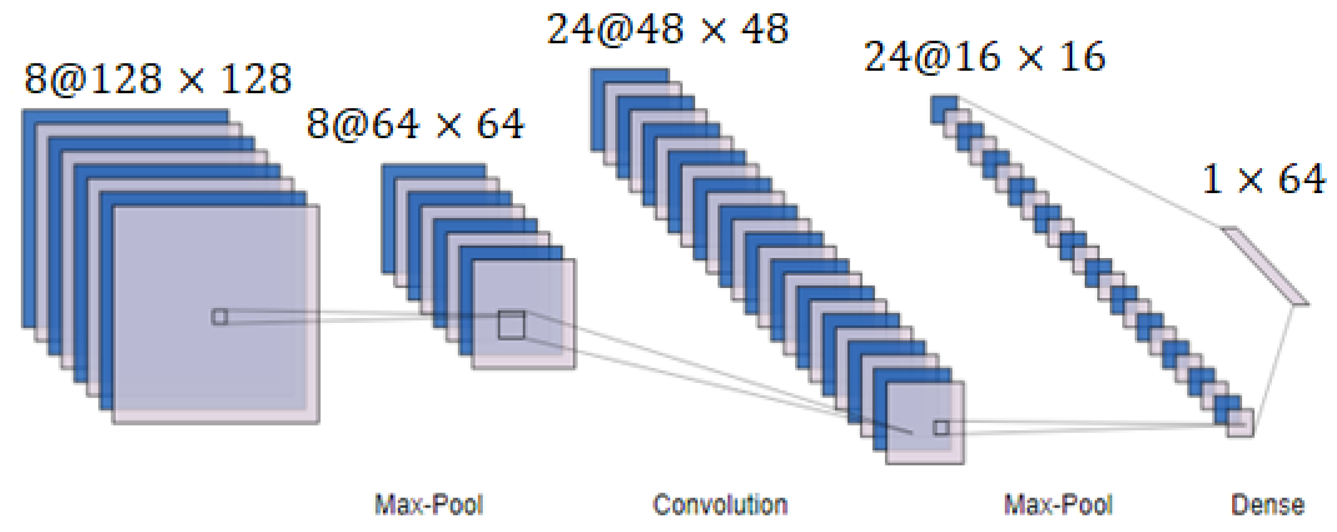
3.1. Convolutional Neural Networks
3.2. Residual Neural Networks
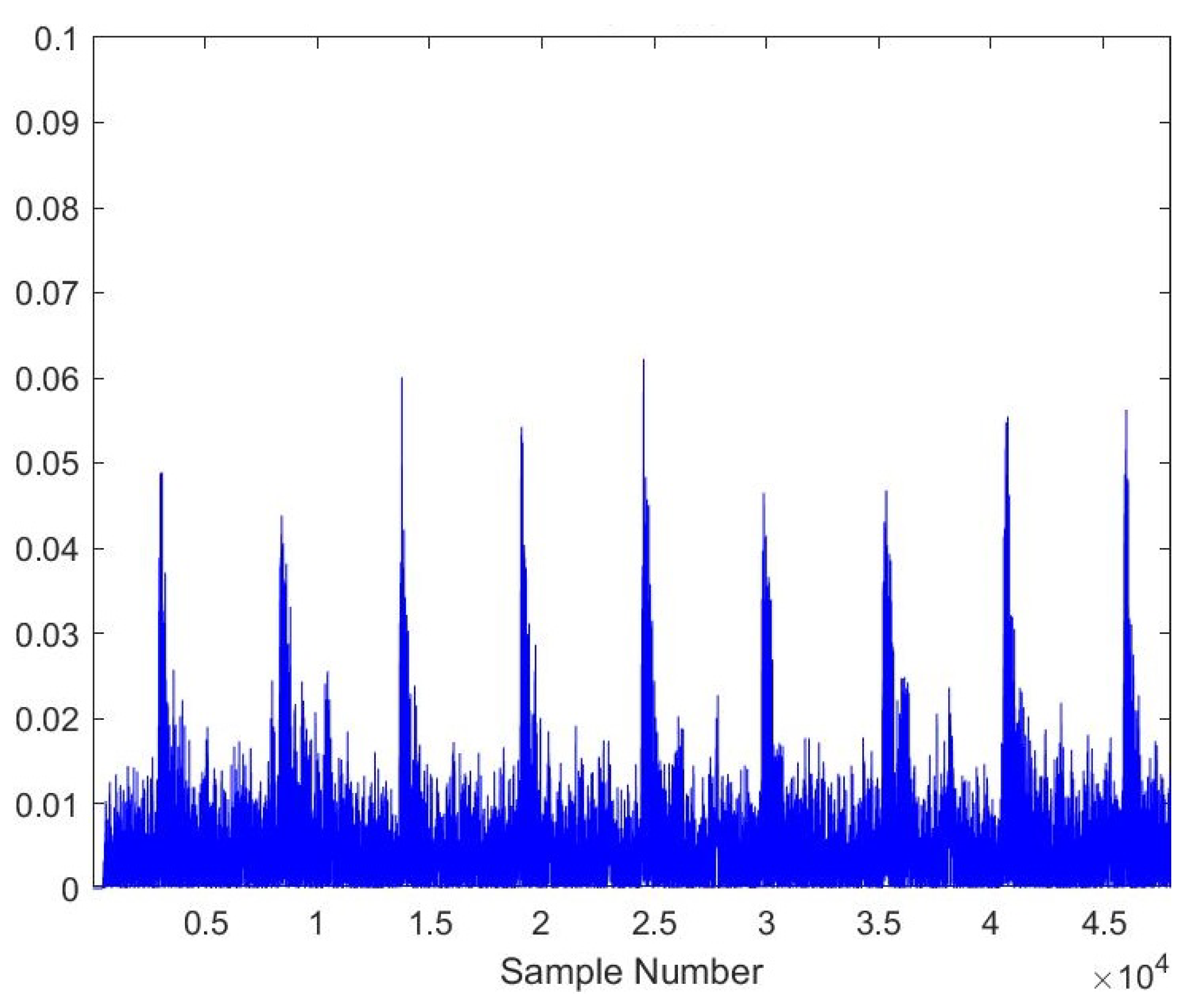
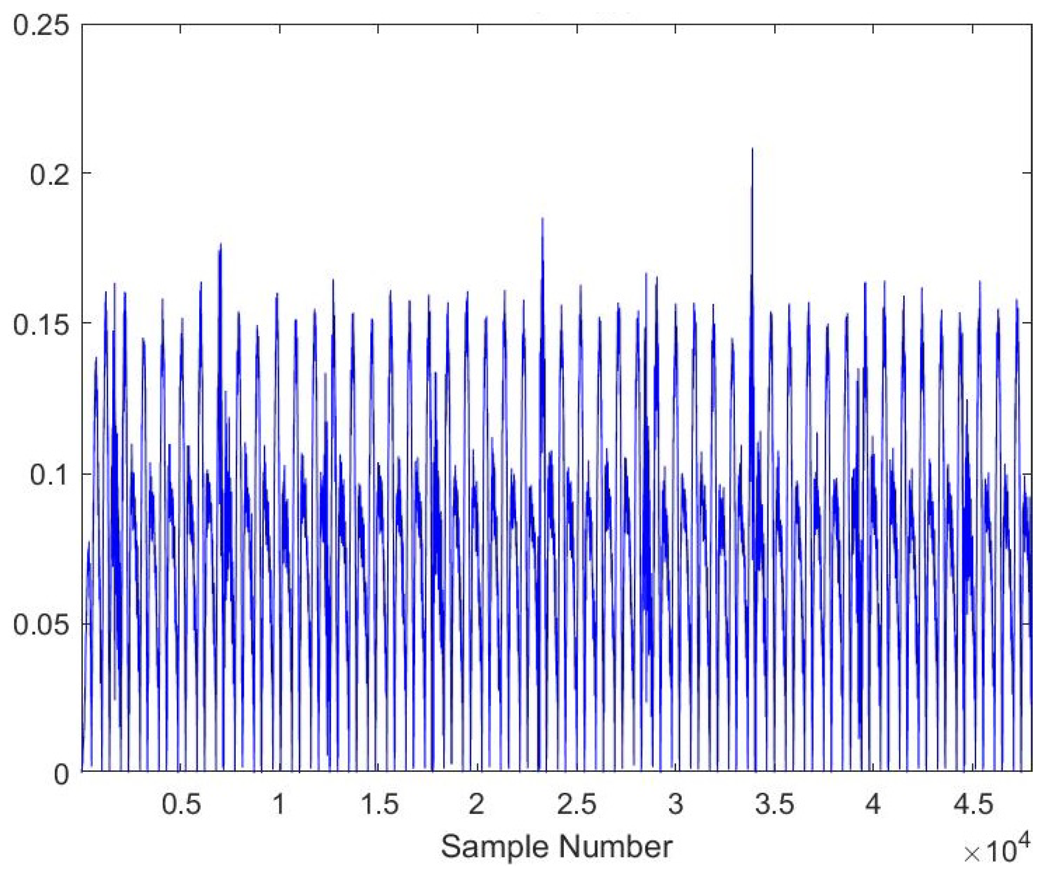
3.3. Experimental Procedures and Setup
4. Results
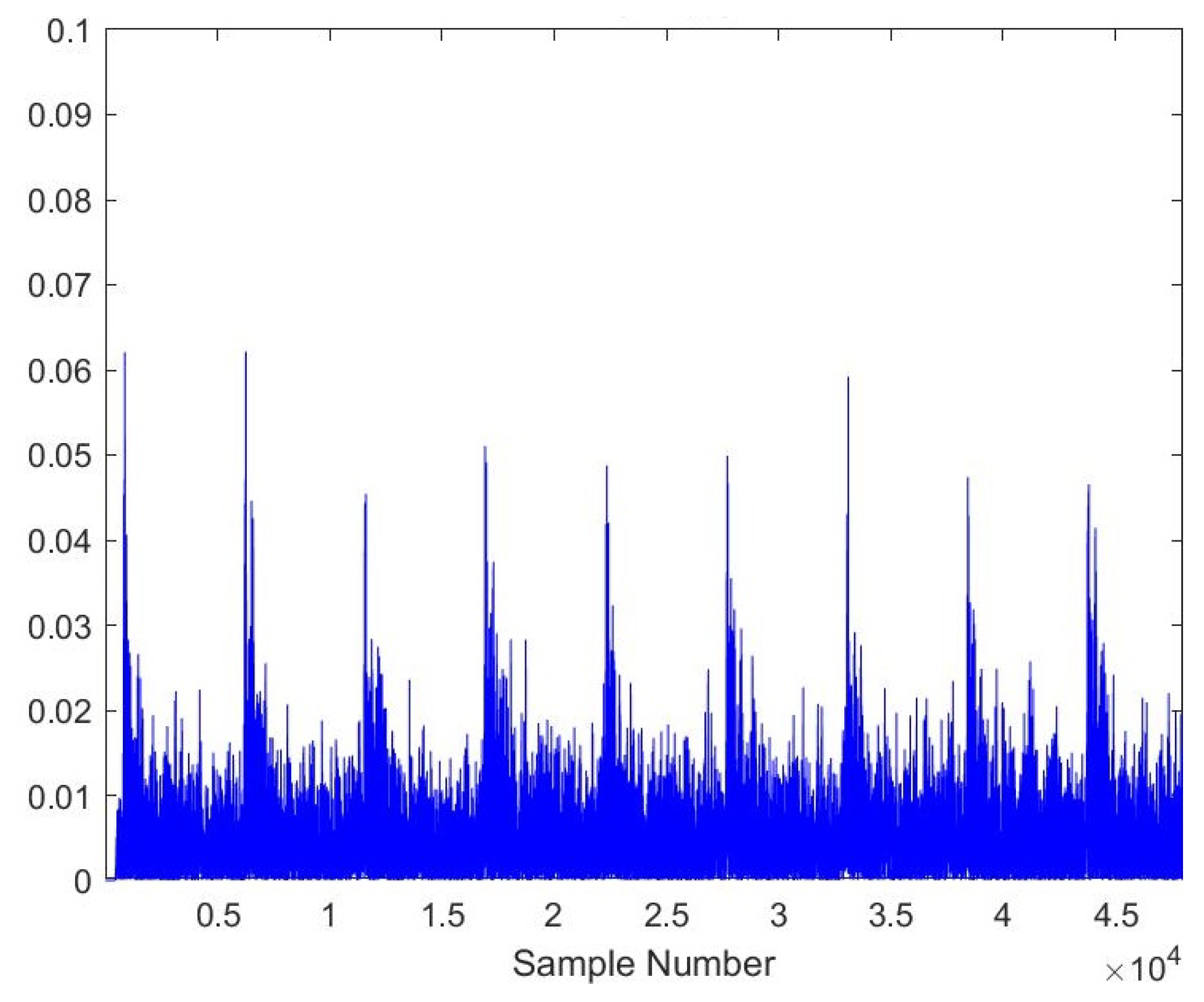
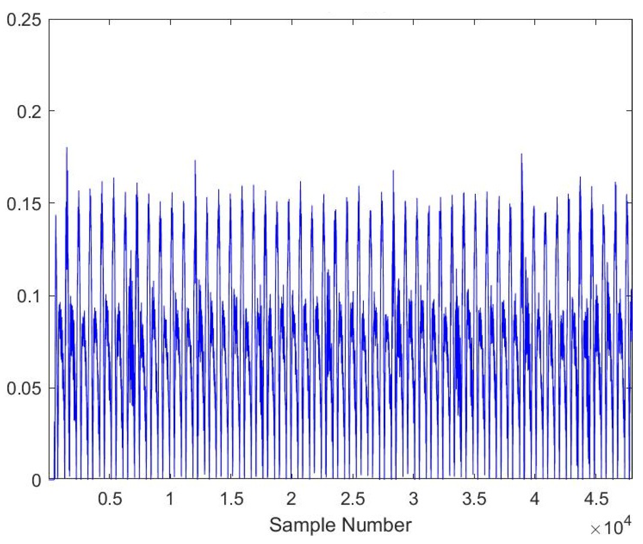
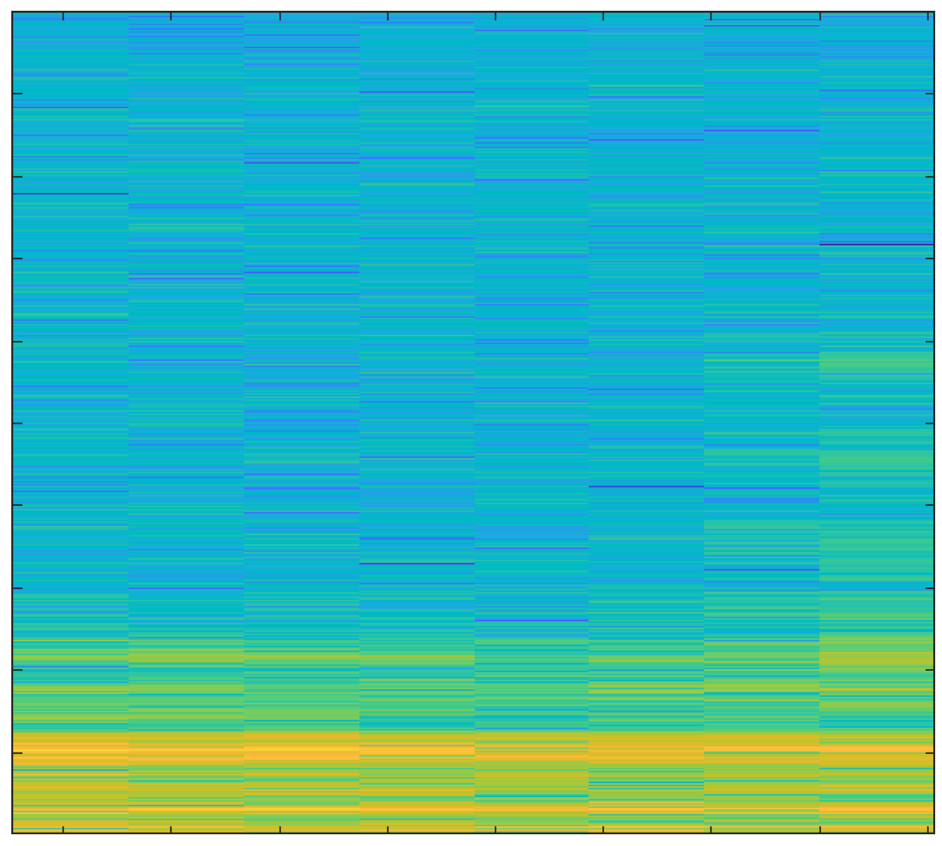
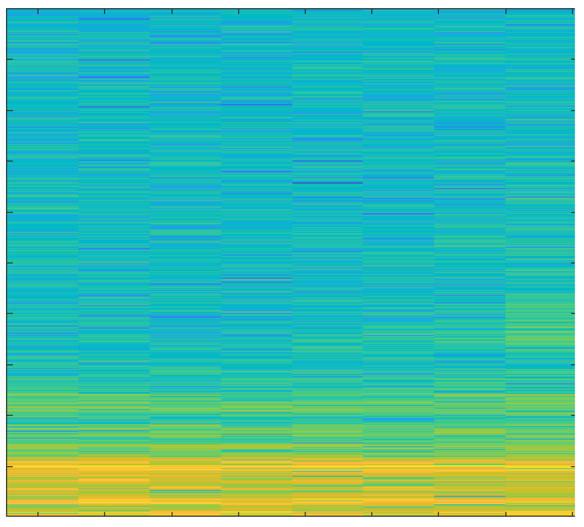
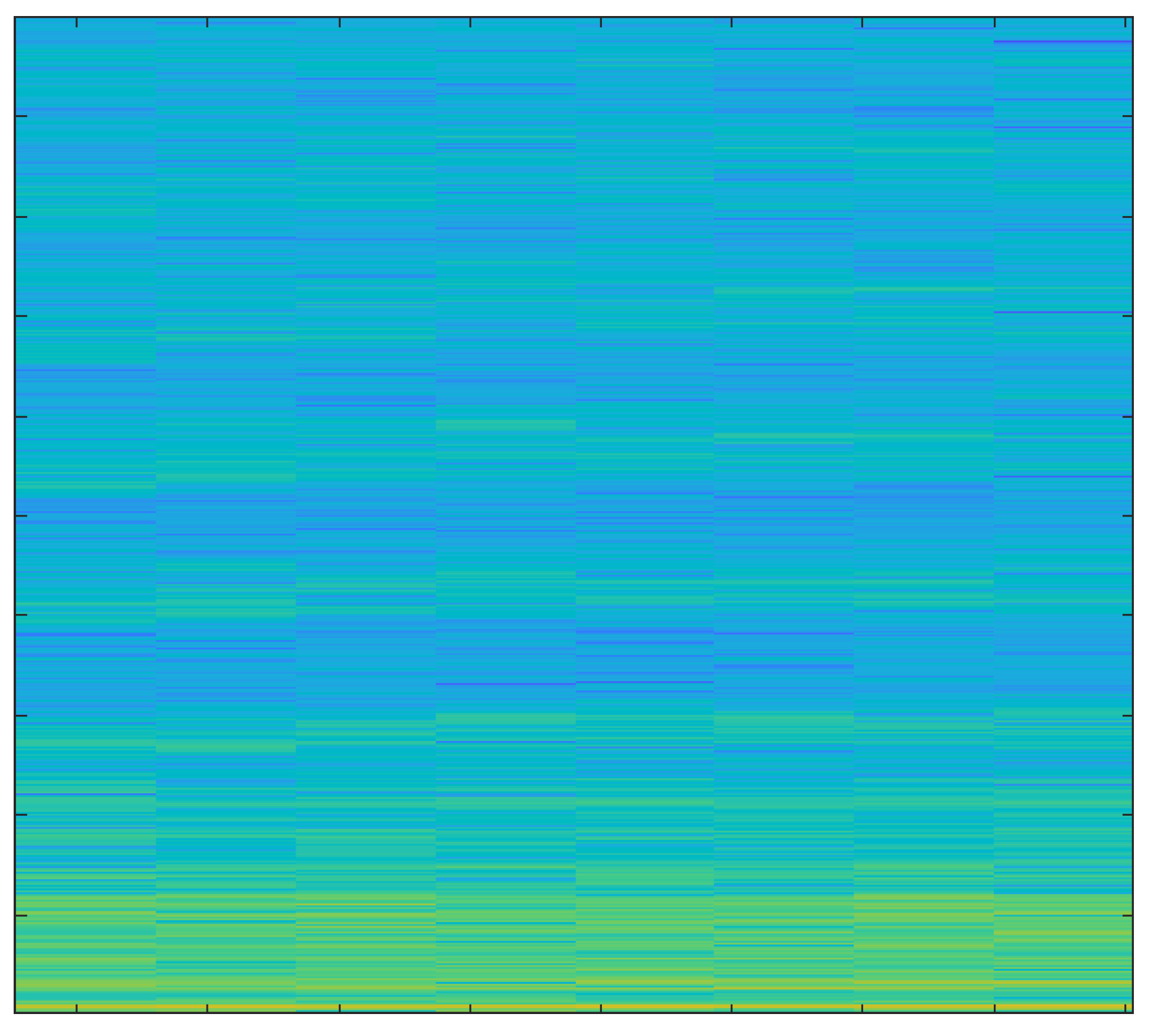
Spectrograms
5. Discussion
6. Conclusions
- The proposed model can be enhanced further by gathering more relevant data from the industry and training the model on that data to develop a comprehensive system according to industry needs.
- The training time of the model can be further reduced by incorporating computers with high-end GPUs which are used for training deep learning models.
- A better-quality microphone can be incorporated which is able to catch more ranges of frequency and has the built-in feature of active noise cancellation.
- Comprehensive understanding of the tool’s health can be considered.
- Testing the model on a wider variety of machines and tools to increase its generalizability to different industrial settings.
- Investigating the use of other machine learning algorithms and techniques, such as deep reinforcement learning, to improve the model’s accuracy and performance.
- Developing a real-time monitoring system that can be integrated into industrial processes to provide real-time notifications of tool wear.
- Conducting further research to investigate the potential of using AE signals for monitoring other types of machinery and equipment in industrial settings.
- Developing a cost–benefit analysis to determine the financial advantages of implementing this method in industrial settings.
- Conducting case studies with industrial partners to validate the proposed method in real-world scenarios.
- Developing a user-friendly interface to make it easier for operators to interpret the results and take appropriate actions.
- Investigate the possibility of incorporating other parameters to improve the model’s ability to identify the wear state of the tools.
Author Contributions
Funding
Institutional Review Board Statement
Informed Consent Statement
Data Availability Statement
Acknowledgments
Conflicts of Interest
References
- ISA Interchange. World’s Largest Manufacturers Lose $1 Trillion/Year to Machine Failure. 2022. Available online: https://blog.isa.org/worlds-largest-manufacturers-lose-1-trillion/year-to-machine-failure. (accessed on 2 January 2023).
- McHatton, D. 10 Ways Preventative Maintenance Can Assist in Reducing Downtime. 2017. Available online: https://www.sageautomation.com/blog/10-ways-preventative-maintenance-can-assist-in-reducing-downtime (accessed on 2 January 2023).
- Unlocking Performance How Manufacturers Can Achieve Top Quartile Performance. 2022. Available online: https://partners.wsj.com/emerson/unlocking-performance/how-manufacturers-can-achieve-top-quartile-performance/ (accessed on 2 January 2023).
- Top Ten Causes of Financial Loss for Businesses. 2018. Available online: https://www.sherwininsurance.co.uk/2018/07/20/top-ten-causes-of-financial-loss-for-businesses/ (accessed on 2 January 2023).
- Nath, C. Integrated Tool Condition Monitoring Systems and Their Applications: A Comprehensive Review. Procedia Manuf. 2020, 48, 852–863. [Google Scholar] [CrossRef]
- Mohamed, A.; Hassan, M.; M’Saoubi, R.; Attia, H. Tool Condition Monitoring for High-Performance Machining Systems—A Review. Sensors 2022, 22, 2206. [Google Scholar] [CrossRef]
- Wang, M.; Wang, J. CHMM for tool condition monitoring and remaining useful life prediction. Int. J. Adv. Manuf. Technol. 2012, 59, 463–471. [Google Scholar] [CrossRef]
- Alonso, F.; Salgado, D. Analysis of the structure of vibration signals for tool wear detection. Mech. Syst. Signal. Process 2008, 22, 735–748. [Google Scholar] [CrossRef]
- Madhusudana, C.K.; Kumar, H.; Narendranath, S. Condition Monitoring of face milling tool using K-star algorithm and histogram features of vibration signal. Eng. Sci. Technol. Int. J. 2016, 19, 1543–1551. [Google Scholar] [CrossRef]
- Sundaram, S.; Senthilkumar, P.; Kumaravel, A.; Manoharan, N. Study of flank wear in single point cutting tool using acoustic emission sensor techniques. ARPN J. Eng. Appl. Sci. 2008, 3, 32–36. [Google Scholar]
- Da Silva, R.H.L.; da Silva, M.B.; Hassui, A. A probabilistic neural network applied in monitoring tool wear in the end milling operation via acoustic emission and cutting power signals. Mach. Sci. Technol. 2016, 20, 386–405. [Google Scholar] [CrossRef]
- Krishnakumar, P.; Rameshkumar, K.; Ramachandran, K.I. Machine learning based tool condition classification using acoustic emission and vibration data in high speed milling process using wavelet features. Intel. Decis. Technol. 2018, 12, 265–282. [Google Scholar] [CrossRef]
- Wang, C.; Bao, Z.; Zhang, P.; Ming, W.; Chen, M. Tool wear evaluation under minimum quantity lubrication by clustering energy of acoustic emission burst signals. Measurement 2019, 138, 256–265. [Google Scholar] [CrossRef]
- Cuka, B.; Kim, D.-W. Fuzzy logic based tool condition monitoring for end-milling. Robot. Comput. Integr. Manuf. 2017, 47, 22–36. [Google Scholar] [CrossRef]
- Arslan, M.; Kamal, K.; Sheikh, M.F.; Khan, M.A.; Ratlamwala, T.A.H.; Hussain, G.; Alkahtani, M. Tool Health Monitoring Using Airborne Acoustic Emission and Convolutional Neural Networks: A Deep Learning Approach. Appl. Sci. 2021, 11, 2734. [Google Scholar] [CrossRef]
- Rangwala, S.; Dornfeld, D. Sensor integration using neural networks for intelligent tool condition monitoring. J. Eng. Ind. 1990, 112, 219–228. [Google Scholar] [CrossRef]


| Researcher | Approach | Application | Accuracy |
|---|---|---|---|
| Madhusudana [9] | K-star Algorithm | Fault diagnosis of tools in face milling | 96% |
| R. H. L. Da Silva et al. [11] | Probabilistic Neural Network | Tool life prediction using AE and cutting power signals | 91% |
| P. Krishnakumar et al. [12] | Support Vector Machines | High-speed precision machining of a titanium alloy | 99.26% |
| M. Arsalan et al. [15] | Convolutional Neural Network | Tool life prediction while working on Teflon, mild steel, and aluminum workpieces | 99% |
| S. Rangwala and D. Dornfeld [16] | Artificial Neural Network | Tool health prediction using noisy signals | 95% |
| Proposed Approach | Residual Neural Network | Wood-milling machining process on hard and soft wood | 100% (hardwood) 99.5% (softwood) |
| Tree Name | Biological Name | Specific Gravity | Modulus of Rupture | Density |
|---|---|---|---|---|
| Pine (Hard) | Pinus | 0.40 | 64.1 MPa | 430–570 kg/m3 |
| Himalayan Spruce (Soft) | Picea Smithiana | 0.39 | 39 MPa | 333–365 kg/m3 |
| Residual Block Number | Size of Filter | Number of Filters | Number of Convolutional Layers |
|---|---|---|---|
| 1 | 3 × 3 | 64 | 1 |
| 2 | 3 × 3 | 64 | 4 |
| 3 | 3 × 3 | 128 | 4 |
| 4 | 3 × 3 | 256 | 4 |
| 5 | 3 × 3 | 512 | 4 |
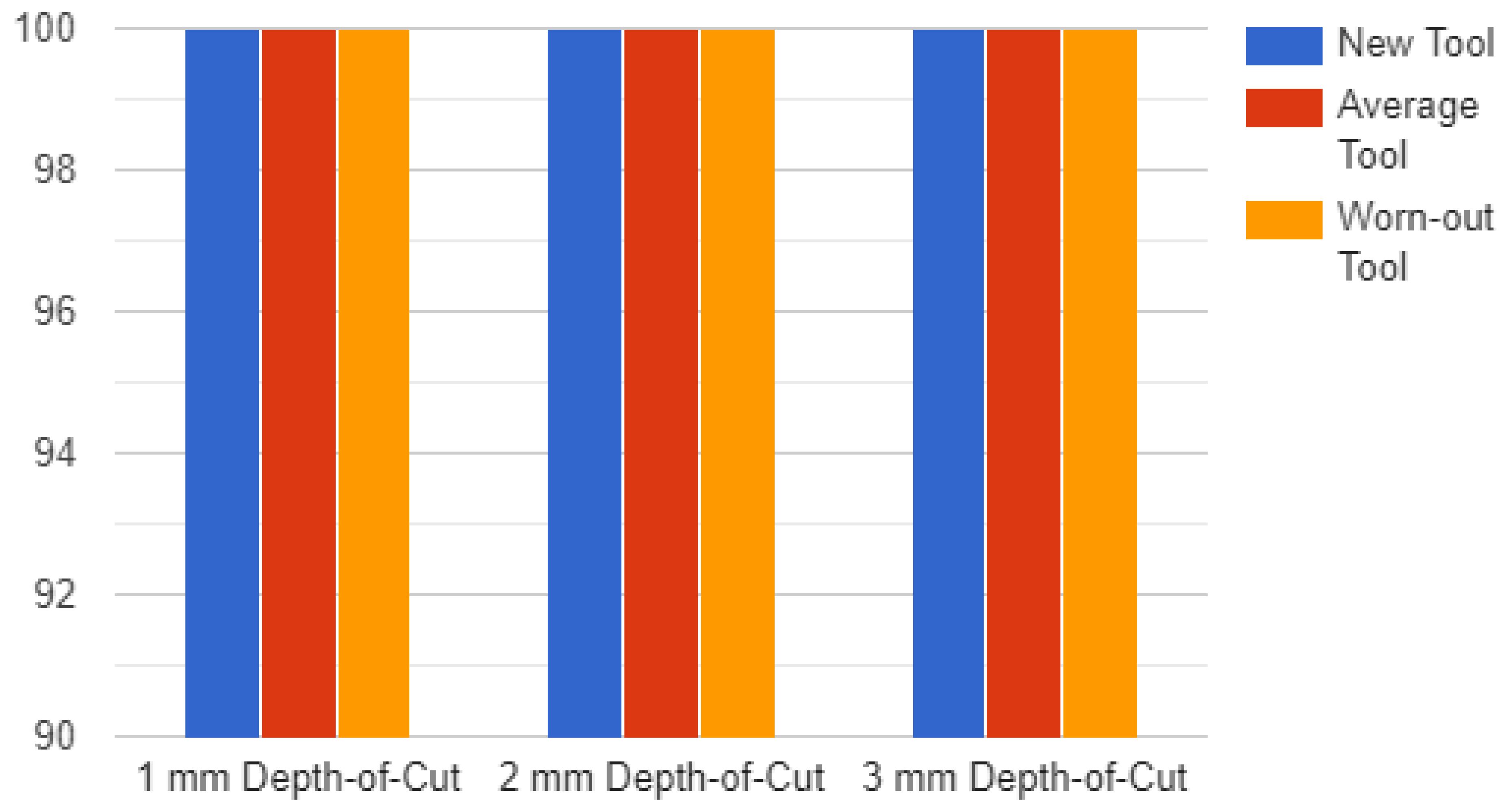
| Work Pieces Types | Performance Parameter | New Tool | Average Tool | Worn-Out Tool | Average |
|---|---|---|---|---|---|
| Hardwood, 1 mm depth-of-cut | Accuracy | 100% | 100% | 100% | 100% |
| Precision | 100% | 100% | 100% | 100% | |
| Recall | 100% | 100% | 100% | 100% | |
| F-score | 100% | 100% | 100% | 100% | |
| Hardwood, 2 mm depth-of-cut | Accuracy | 100% | 100% | 100% | 100% |
| Precision | 100% | 100% | 100% | 100% | |
| Recall | 100% | 100% | 100% | 100% | |
| F-score | 100% | 100% | 100% | 100% | |
| Hardwood, 3 mm depth-of-cut | Accuracy | 100% | 100% | 100% | 100% |
| Precision | 100% | 100% | 100% | 100% | |
| Recall | 100% | 100% | 100% | 100% | |
| F-score | 100% | 100% | 100% | 100% | |
| Softwood, 1 mm depth-of-cut | Accuracy | 100% | 100% | 99.7% | 99.9% |
| Precision | 100% | 100% | 100% | 100% | |
| Recall | 100% | 100% | 94.8% | 98.2% | |
| F-score | 100% | 100% | 97.3% | 99.1% | |
| Softwood, 2 mm depth-of-cut | Accuracy | 100% | 100% | 100% | 100% |
| Precision | 100% | 100% | 100% | 100% | |
| Recall | 100% | 100% | 100% | 100% | |
| F-score | 100% | 100% | 100% | 100% | |
| Softwood, 3 mm depth-of-cut | Accuracy | 100% | 99.7% | 100% | 99.9% |
| Precision | 100% | 95.6% | 100% | 98.5% | |
| Recall | 100% | 100% | 100% | 100% | |
| F-score | 100% | 97.7% | 100% | 99.2% |
Disclaimer/Publisher’s Note: The statements, opinions and data contained in all publications are solely those of the individual author(s) and contributor(s) and not of MDPI and/or the editor(s). MDPI and/or the editor(s) disclaim responsibility for any injury to people or property resulting from any ideas, methods, instructions or products referred to in the content. |
© 2023 by the authors. Licensee MDPI, Basel, Switzerland. This article is an open access article distributed under the terms and conditions of the Creative Commons Attribution (CC BY) license (https://creativecommons.org/licenses/by/4.0/).
Share and Cite
Ahmed, M.; Kamal, K.; Ratlamwala, T.A.H.; Hussain, G.; Alqahtani, M.; Alkahtani, M.; Alatefi, M.; Alzabidi, A. Tool Health Monitoring of a Milling Process Using Acoustic Emissions and a ResNet Deep Learning Model. Sensors 2023, 23, 3084. https://doi.org/10.3390/s23063084
Ahmed M, Kamal K, Ratlamwala TAH, Hussain G, Alqahtani M, Alkahtani M, Alatefi M, Alzabidi A. Tool Health Monitoring of a Milling Process Using Acoustic Emissions and a ResNet Deep Learning Model. Sensors. 2023; 23(6):3084. https://doi.org/10.3390/s23063084
Chicago/Turabian StyleAhmed, Mustajab, Khurram Kamal, Tahir Abdul Hussain Ratlamwala, Ghulam Hussain, Mejdal Alqahtani, Mohammed Alkahtani, Moath Alatefi, and Ayoub Alzabidi. 2023. "Tool Health Monitoring of a Milling Process Using Acoustic Emissions and a ResNet Deep Learning Model" Sensors 23, no. 6: 3084. https://doi.org/10.3390/s23063084
APA StyleAhmed, M., Kamal, K., Ratlamwala, T. A. H., Hussain, G., Alqahtani, M., Alkahtani, M., Alatefi, M., & Alzabidi, A. (2023). Tool Health Monitoring of a Milling Process Using Acoustic Emissions and a ResNet Deep Learning Model. Sensors, 23(6), 3084. https://doi.org/10.3390/s23063084