
Advanced Computer Vision-Based Subsea Gas Leaks Monitoring: A Comparison of Two Approaches

 , ,
, ,  ,
,
Abstract
1. Introduction
2. Theory of Two Advanced Computer Vision-Based Detection Approaches
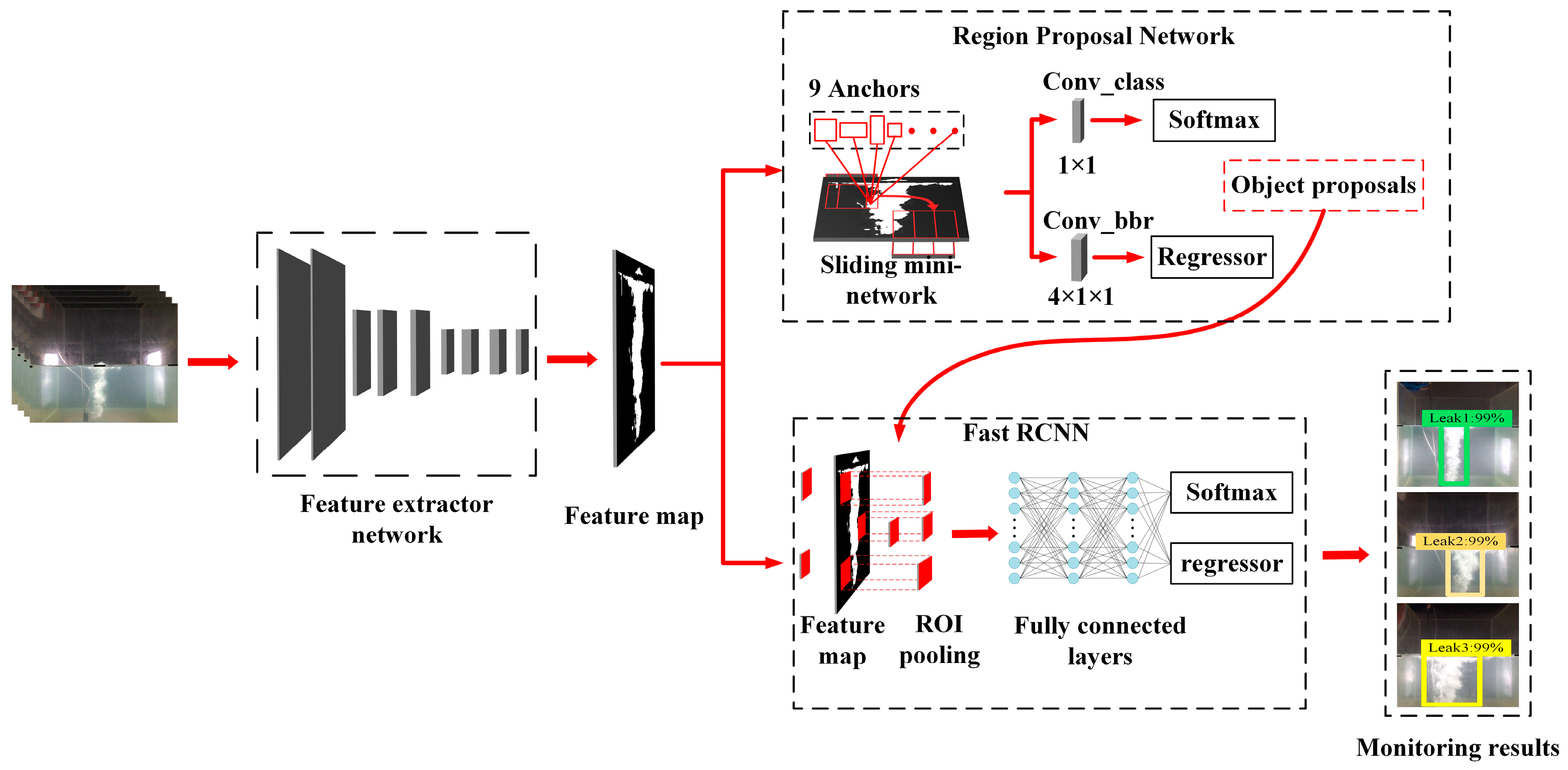
2.1. Faster R-CNN Approach
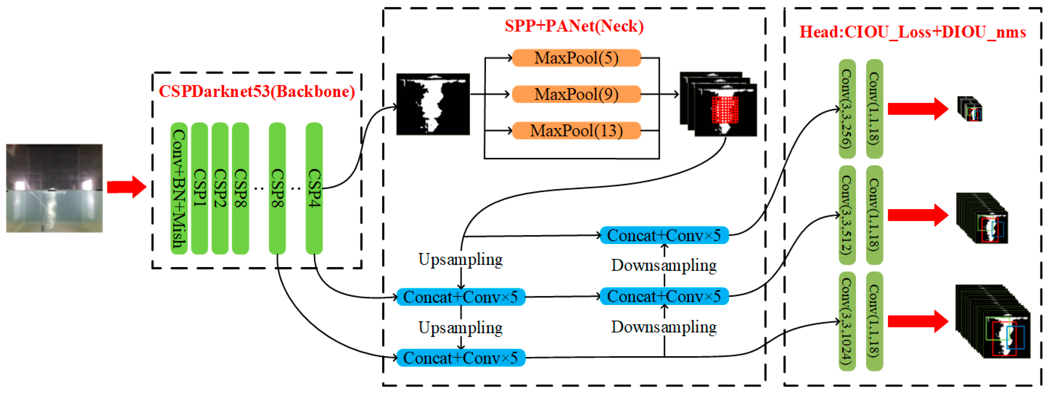
2.2. YOLOv4 Approach
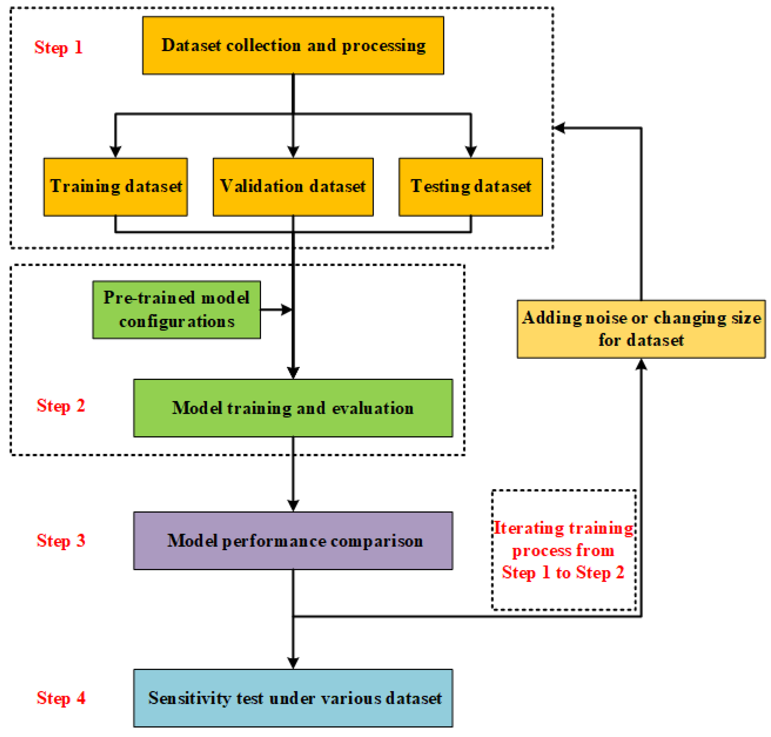
3. Methodology to Develop an Optimal Gas Leakage Monitoring Model
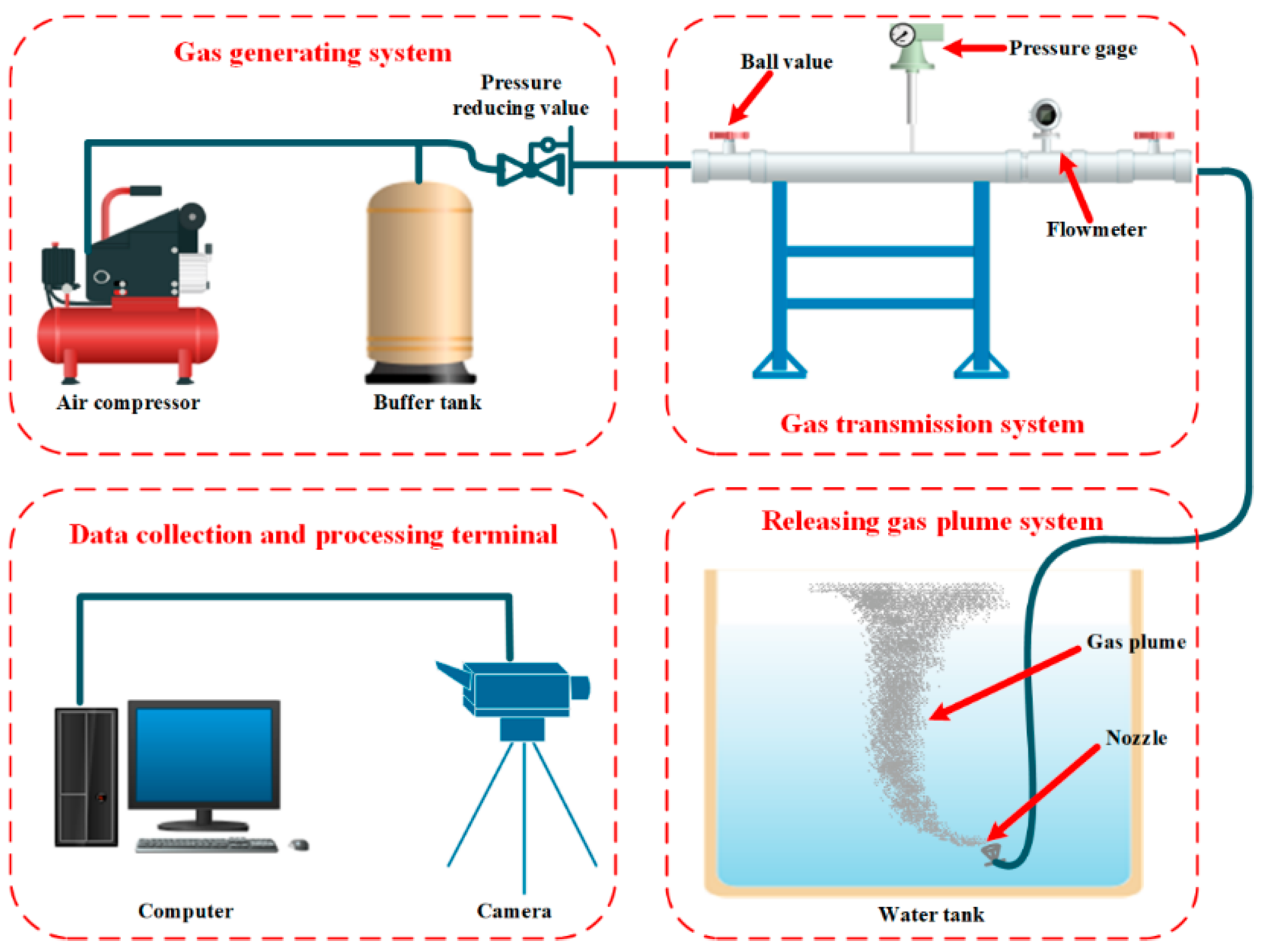
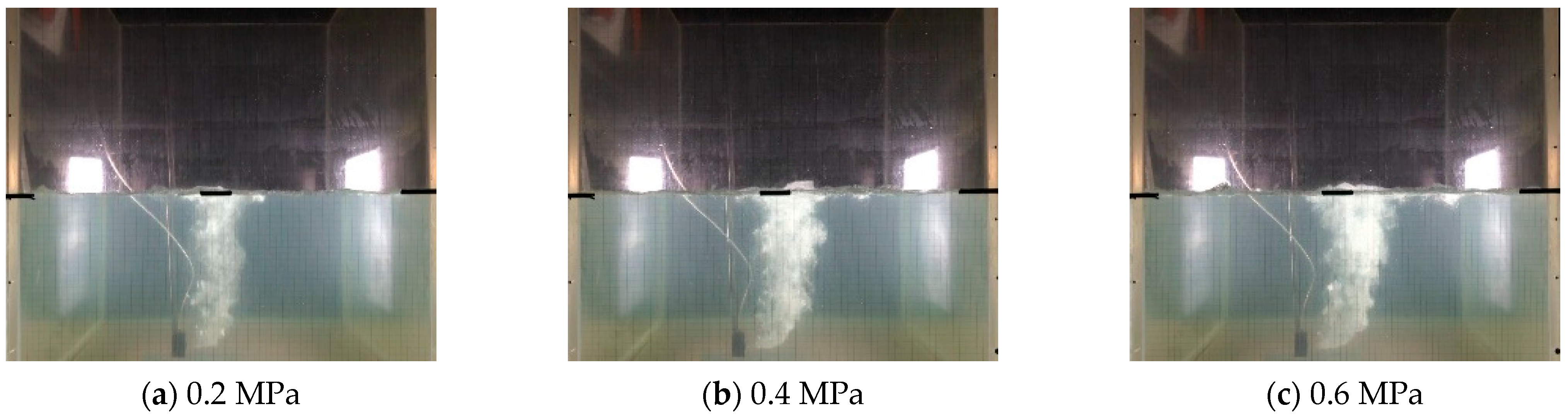
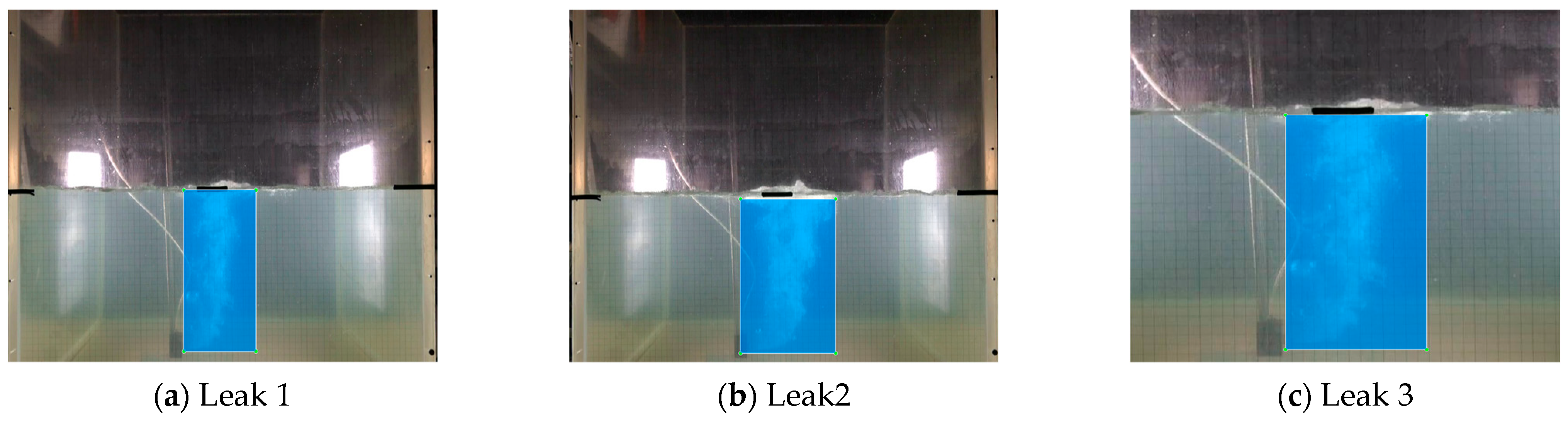
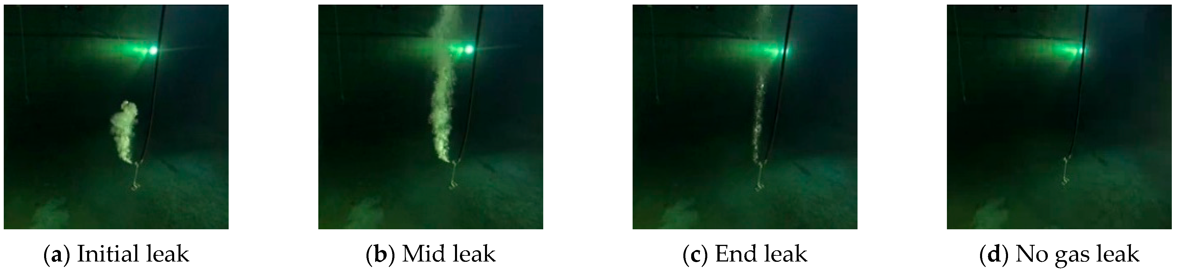
4. Collection Datasets Concerning Underwater Gas Leakage Plume
5. Results and Discussion
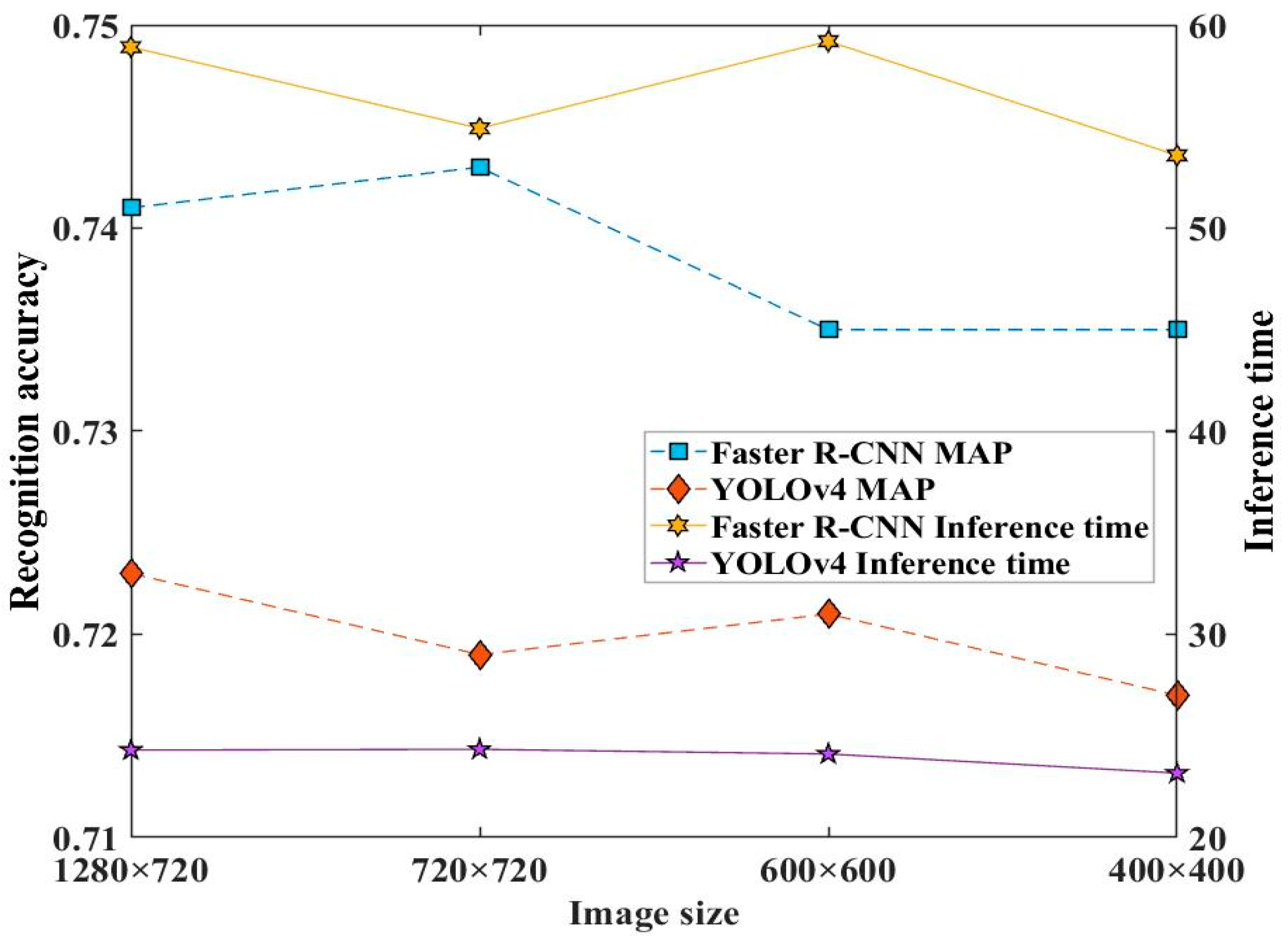
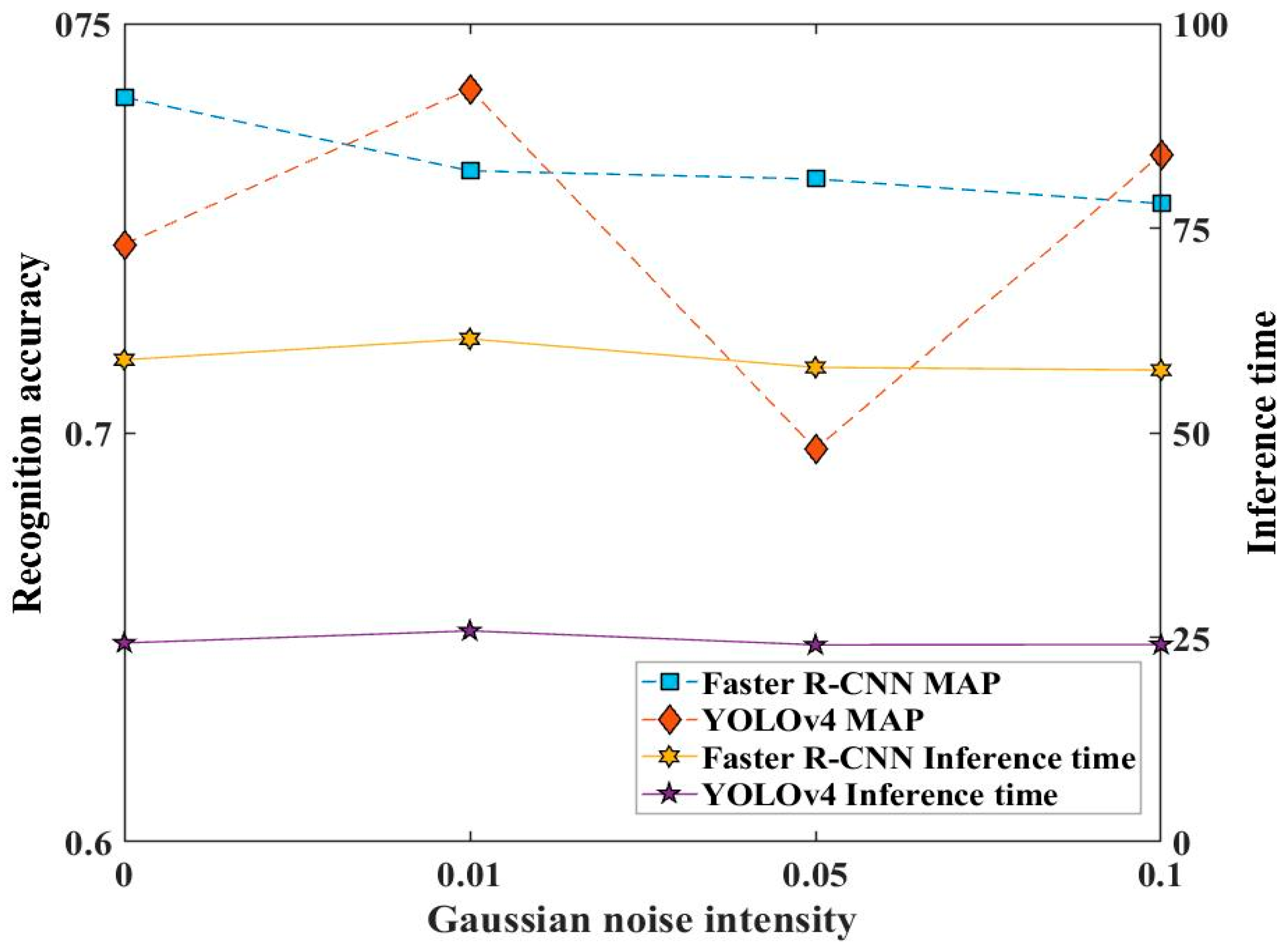
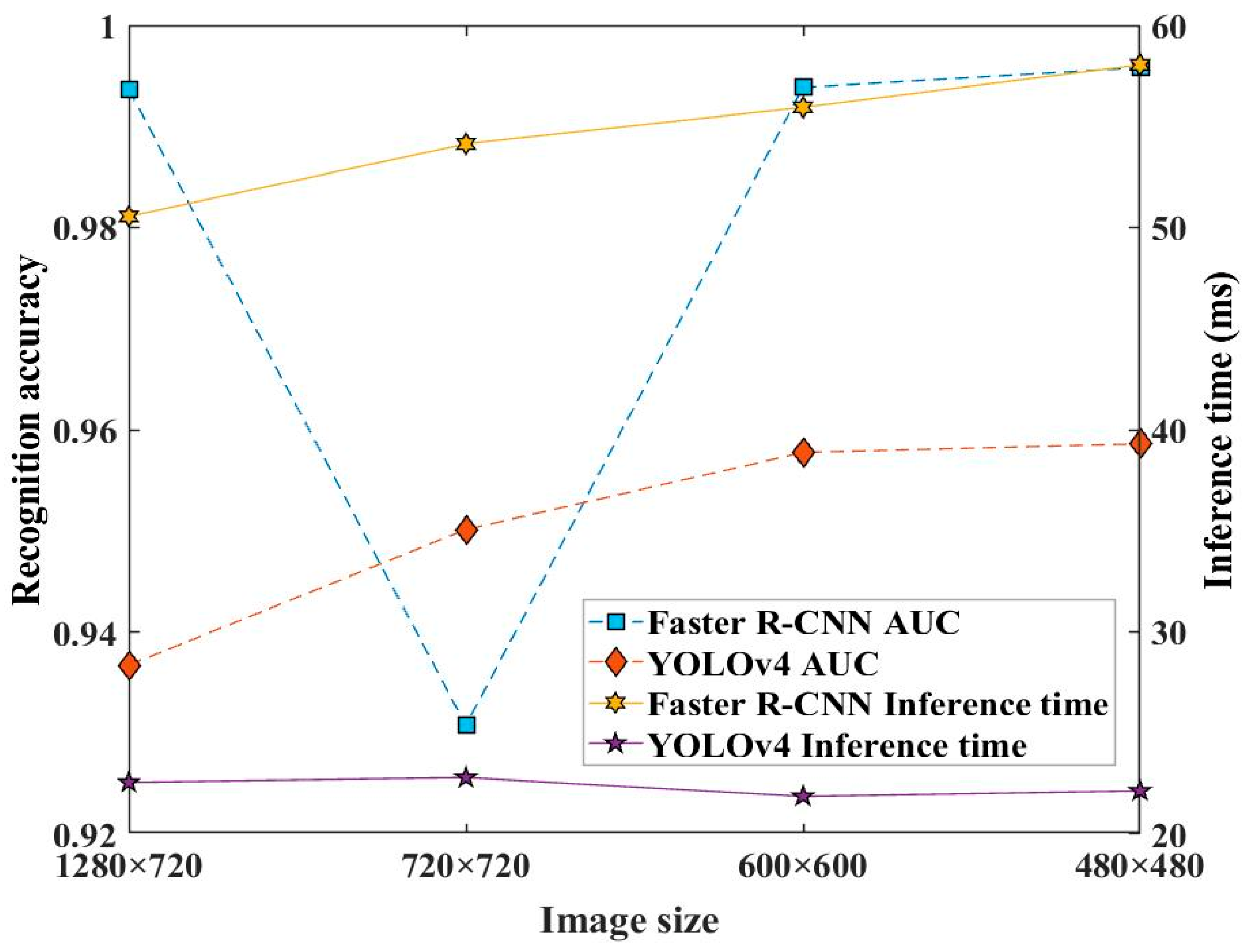
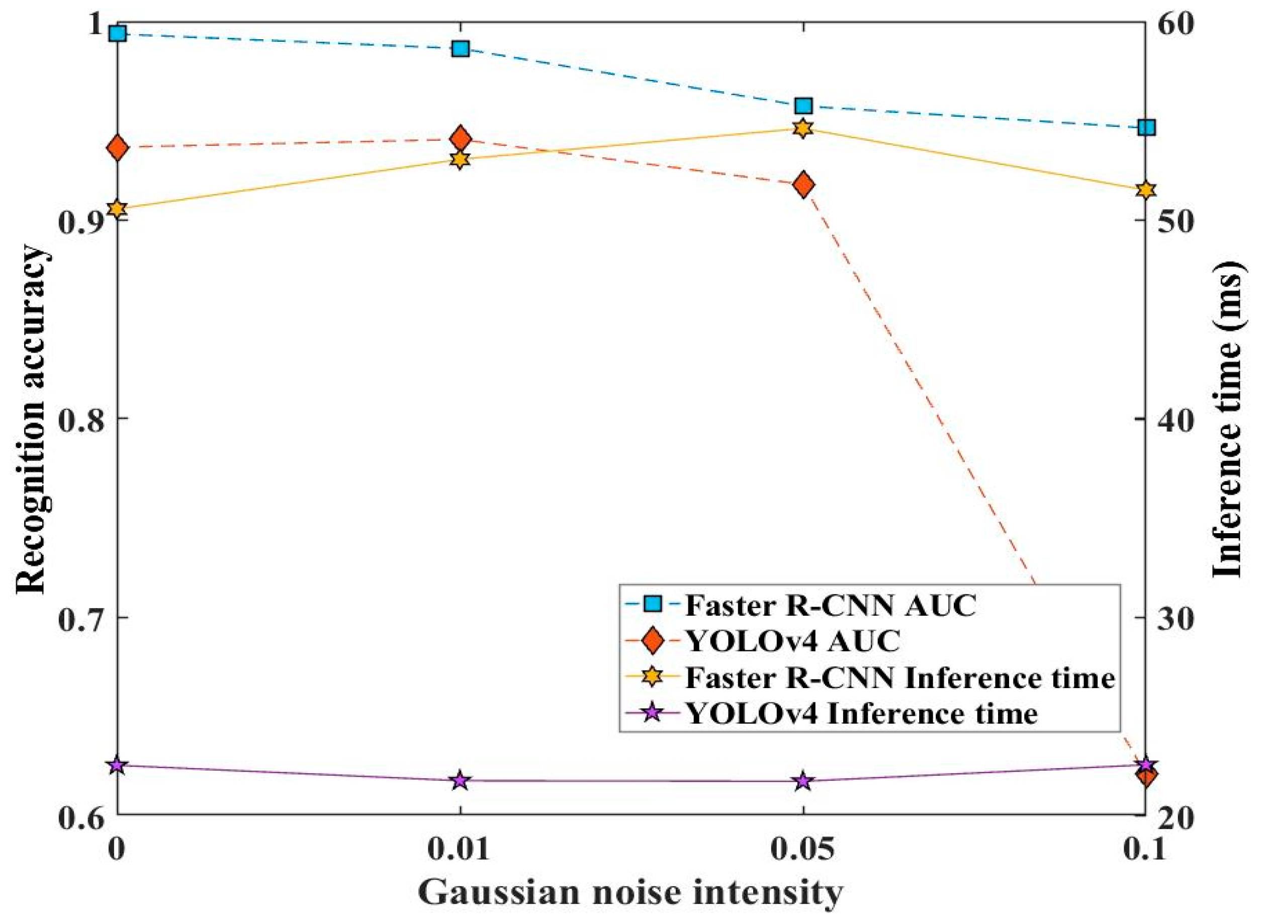
5.1. Monitoring Performance Comparison of Two Approaches under Experimental Datasets
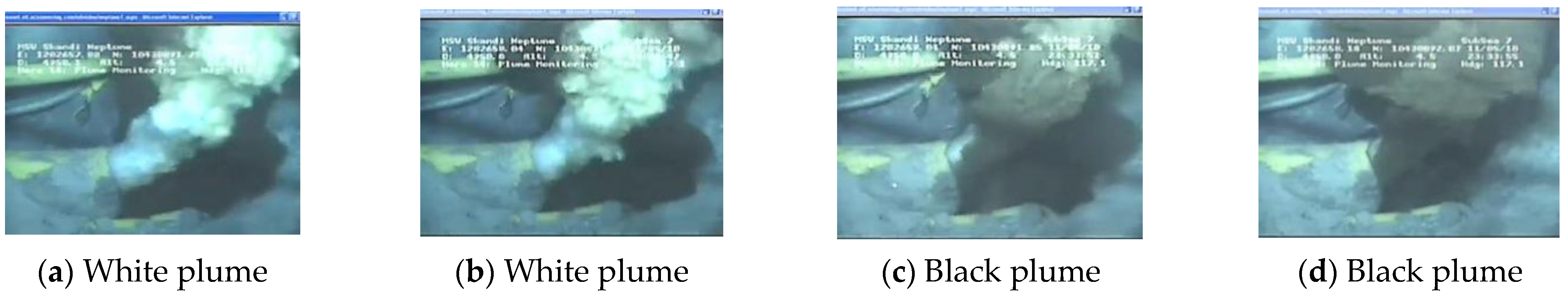
5.2. Monitoring Performance Comparison of Two Approaches under Real-World Datasets
5.3. Comparison between Faster R-CNN Model and YOLOv4 Model under Real World Datasets
6. Conclusions
Author Contributions
Funding
Institutional Review Board Statement
Informed Consent Statement
Data Availability Statement
Conflicts of Interest
References
- Olsen, J.E.; Skjetne, P. Current understanding of subsea gas release: A review. Can. J. Chem. Eng. 2016, 94, 209–219. [Google Scholar] [CrossRef]
- Dadashzadeh, M.; Abbassi, R.; Khan, F.; Hawboldt, K. Explosion modeling and analysis of BP Deepwater Horizon accident. Saf. Sci. 2013, 57, 150–160. [Google Scholar] [CrossRef]
- Lee, J.D.; Mobbs, S.D.; Wellpott, A.; Allen, G.; Bauguitte, S.J.B.; Burton, R.R.; Camilli, R.; Coe, H.; Fisher, R.E.; France, J.L.; et al. Flow rate and source reservoir identification from airborne chemical sampling of the uncontrolled Elgin platform gas release. Atmos. Meas. Tech. 2018, 11, 1725–1739. [Google Scholar] [CrossRef]
- Li, X.; Khan, F.; Yang, M.; Chen, C.; Chen, G. Risk assessment of offshore fire accidents caused by subsea gas release. Appl. Ocean Res. 2021, 115, 102828. [Google Scholar] [CrossRef]
- Li, X.; Chen, G.; Khan, F. Analysis of underwater gas release and dispersion behavior to assess subsea safety risk. J. Hazard. Mater. 2019, 367, 676–685. [Google Scholar] [CrossRef] [PubMed]
- Premathilake, L.T.; Yapa, P.D.; Nissanka, I.D.; Kumarage, P. Impact on water surface due to deepwater gas blowouts. Mar. Pollut. Bull. 2016, 112, 365–374. [Google Scholar] [CrossRef]
- Glasby, G.P. Potential impact on climate of the exploitation of methane hydrate deposits offshore. Mar. Pet. Geol. 2003, 20, 163–175. [Google Scholar] [CrossRef]
- Bucelli, M.; Utne, I.B.; Salvo Rossi, P.; Paltrinieri, N. A system engineering approach to subsea spill risk management. Saf. Sci. 2020, 123, 104560. [Google Scholar] [CrossRef]
- Kita, J.; Stahl, H.; Hayashi, M.; Green, T.; Watanabe, Y.; Widdicombe, S. Benthic megafauna and CO2 bubble dynamics observed by underwater photography during a controlled sub-seabed release of CO2. Int. J. Greenh. Gas Control 2015, 38, 202–209. [Google Scholar] [CrossRef]
- Pham, L.H.H.P.; Rusli, R.; Shariff, A.M.; Khan, F. Dispersion of carbon dioxide bubble release from shallow subsea carbon dioxide storage to seawater. Cont. Shelf Res. 2020, 196, 104075. [Google Scholar] [CrossRef]
- Cazenave, P.W.; Dewar, M.; Torres, R.; Blackford, J.; Bedington, M.; Artioli, Y.; Bruggeman, J. Optimising environmental monitoring for carbon dioxide sequestered offshore. Int. J. Greenh. Gas Control 2021, 110, 103397. [Google Scholar] [CrossRef]
- Flohr, A.; Schaap, A.; Achterberg, E.P.; Alendal, G.; Arundell, M.; Berndt, C.; Blackford, J.; Böttner, C.; Borisov, S.M.; Brown, R.; et al. Towards improved monitoring of offshore carbon storage: A real-world field experiment detecting a controlled sub-seafloor CO2 release. Int. J. Greenh. Gas Control 2021, 106, 103237. [Google Scholar] [CrossRef]
- Barbagelata, L.; Kostianoy, A.G. Co.L.Mar.: Subsea Leak Detection with Passive Acoustic Technology. In Oil and Gas Pipelines in the Black-Caspian Seas Region; Zhiltsov, S.S., Zonn, I.S., Kostianoy, A.G., Eds.; Springer International Publishing: Cham, Germany, 2016; pp. 261–277. [Google Scholar]
- Vrålstad, T.; Melbye, A.G.; Carlsen, I.M.; Llewelyn, D. Comparison of Leak-Detection Technologies for Continuous Monitoring of Subsea-Production Templates. SPE Proj. Facil. Constr. 2011, 6, 96–103. [Google Scholar] [CrossRef]
- Eisler, B.; Lanan, G.A. Fiber optic leak detection systems for subsea pipelines. In Proceedings of the Offshore Technology Conference, Houston, TX, USA, 30 April–3 May 2012. [Google Scholar]
- Wang, Q.; Wang, X. Interferometeric fibre optic signal processing based on wavelet transform for subsea gas pipeline leakage inspection. In Proceedings of the 2010 International Conference on Measuring Technology and Mechatronics Automation, Changsha, China, 13–14 March 2010; IEEE: New York, NY, USA, 2010; pp. 501–504. [Google Scholar]
- McStay, D.; Kerlin, J.; Acheson, R. An optical sensor for the detection of leaks from subsea pipelines and risers. J. Phys. Conf. Ser. 2007, 76, 012009. [Google Scholar] [CrossRef]
- Moodie, D.; Costello, L.; McStay, D. Optoelectronic leak detection system for monitoring subsea structures. In Proceedings of the Subsea Control and Data Acquisition (SCADA) Conference, Newcastle, UK, 2–3 June 2010. [Google Scholar]
- Mahmutoglu, Y.; Turk, K. Positioning of leakages in underwater natural gas pipelines for time-varying multipath environment. Ocean Eng. 2020, 207, 107454. [Google Scholar] [CrossRef]
- DNV. Selection and use of subsea leak detection systems. In Recommended Practice Det Norske Veritas DNV-RP-F302; DNV: Veritasveien, Norway, 2010; Available online: https://naxystech.com/wp-content/uploads/2021/11/RP-F302.pdf (accessed on 2 December 2022).
- Ofualagba, G. Subsea Crude Oil Spill Detection Using Robotic Systems. Eur. J. Eng. Technol. Res. 2019, 4, 112–116. [Google Scholar]
- Murvay, P.-S.; Silea, I. A survey on gas leak detection and localization techniques. J. Loss Prev. Process Ind. 2012, 25, 966–973. [Google Scholar] [CrossRef]
- Huang, Y.; Wang, Q.; Shi, L.; Yang, Q. Underwater gas pipeline leakage source localization by distributed fiber-optic sensing based on particle swarm optimization tuning of the support vector machine. Appl. Opt. 2016, 55, 242–247. [Google Scholar] [CrossRef] [PubMed]
- Boelmann, J.; Zielinski, O. Characterization and quantification of hydrocarbon seeps by means of subsea imaging. In Proceedings of the 2014 Oceans-St. John’s, St. John’s, NL, Canada, 14–19 September 2014; pp. 1–6. [Google Scholar]
- Agbakwuru, J.A.; Gudmestad, O.T.; Groenli, J.G.; Skjaveland, H. Development of Method/Apparatus for Close-Visual Inspection of Underwater Structures (Especially Pipelines) in Muddy and Unclear Water Condition. In Proceedings of the International Conference on Offshore Mechanics and Arctic Engineering, Rotterdam, The Netherlands, 19–24 June 2011; pp. 209–217. [Google Scholar]
- Agbakwuru, J. Oil/Gas pipeline leak inspection and repair in underwater poor visibility conditions: Challenges and perspectives. J. Environ. Prot. 2012, 3, 19510. [Google Scholar]
- Agbakwuru, J.A.; Gudmestad, O.T.; Groenli, J.; Skjæveland, H. Tracking of Buoyancy Flux of Underwater Plumes for Identification, Close Visual Inspection and Repair of Leaking Underwater Pipelines in Muddy Waters. In International Conference on Offshore Mechanics and Arctic Engineering; American Society of Mechanical Engineers: New York, NY, USA, 2013; p. V04ATA002. [Google Scholar]
- Kato, N.; Choyekh, M.; Dewantara, R.; Senga, H.; Chiba, H.; Kobayashi, E.; Yoshie, M.; Tanaka, T.; Short, T. An autonomous underwater robot for tracking and monitoring of subsea plumes after oil spills and gas leaks from seafloor. J. Loss Prev. Process Ind. 2017, 50, 386–396. [Google Scholar] [CrossRef]
- Choyekh, M.; Kato, N.; Yamaguchi, Y.; Dewantara, R.; Chiba, H.; Senga, H.; Yoshie, M.; Tanaka, T.; Kobayashi, E.; Short, T. Development and Operation of Underwater Robot for Autonomous Tracking and Monitoring of Subsea Plumes After Oil Spill and Gas Leak from Seabed and Analyses of Measured Data. In Applications to Marine Disaster Prevention; Springer: Berlin/Heidelberg, Germany, 2017; pp. 17–93. [Google Scholar]
- Matos, A.; Martins, A.; Dias, A.; Ferreira, B.; Almeida, J.M.; Ferreira, H.; Amaral, G.; Figueiredo, A.; Almeida, R.; Silva, F. Multiple robot operations for maritime search and rescue in euRathlon 2015 competition. In Proceedings of the OCEANS 2016-Shanghai, Shanghai, China, 10–13 April 2016; pp. 1–7. [Google Scholar]
- Bonin-Font, F.; Oliver, G.; Wirth, S.; Massot, M.; Negre, P.L.; Beltran, J.-P. Visual sensing for autonomous underwater exploration and intervention tasks. Ocean Eng. 2015, 93, 25–44. [Google Scholar] [CrossRef]
- Boelmann, J.; Zielinski, O. Automated characterization and quantification of hydrocarbon seeps based on frontal illuminated video observations. J. Eur. Opt. Soc. Rapid Publ. 2015, 10, 15018. [Google Scholar] [CrossRef]
- Al-Lashi, R.S.; Gunn, S.R.; Webb, E.G.; Czerski, H. A novel high-resolution optical instrument for imaging oceanic bubbles. IEEE J. Ocean Eng. 2017, 43, 72–82. [Google Scholar] [CrossRef]
- Zhao, J.; Meng, J.; Zhang, H.; Wang, S. Comprehensive detection of gas plumes from multibeam water column images with minimisation of noise interferences. Sensors 2017, 17, 2755. [Google Scholar] [CrossRef] [PubMed]
- Wang, J.; Tchapmi, L.P.; Ravikumar, A.P.; McGuire, M.; Bell, C.S.; Zimmerle, D.; Savarese, S.; Brandt, A.R. Machine vision for natural gas methane emissions detection using an infrared camera. Appl. Energy 2020, 257, 113998. [Google Scholar] [CrossRef]
- Melo, R.O.; Costa, M.G.F.; Costa Filho, C.F.F. Applying Convolutional Neural Networks to Detect Natural Gas Leaks in Wellhead Images. IEEE Access 2020, 8, 191775–191784. [Google Scholar] [CrossRef]
- Jiao, J.; Zhao, M.; Lin, J.; Liang, K. A comprehensive review on convolutional neural network in machine fault diagnosis. Neurocomputing 2020, 417, 36–63. [Google Scholar] [CrossRef]
- Shao, H.; Xia, M.; Han, G.; Zhang, Y.; Wan, J. Intelligent fault diagnosis of rotor-bearing system under varying working conditions with modified transfer convolutional neural network and thermal images. IEEE Trans. Ind. Inform. 2020, 17, 3488–3496. [Google Scholar] [CrossRef]
- Ren, S.; He, K.; Girshick, R.; Sun, J. Faster R-CNN: Towards real-time object detection with region proposal networks. IEEE Trans. Pattern Anal. Mach. Intell. 2016, 39, 1137–1149. [Google Scholar] [CrossRef]
- Liu, W.; Anguelov, D.; Erhan, D.; Szegedy, C.; Reed, S.; Fu, C.-Y.; Berg, A.C. Ssd: Single shot multibox detector. In European Conference on Computer Vision; Springer: Berlin/Heidelberg, Germany, 2016; pp. 21–37. [Google Scholar]
- Bochkovskiy, A.; Wang, C.-Y.; Liao, H.-Y.M. Yolov4: Optimal speed and accuracy of object detection. arXiv 2020, arXiv:2004.10934. [Google Scholar]
- Shi, J.; Chang, B.; Khan, F.; Chang, Y.; Zhu, Y.; Chen, G.; Zhang, C. Stochastic explosion risk analysis of hydrogen production facilities. Int. J. Hydrogen Energy 2020, 45, 13535–13550. [Google Scholar] [CrossRef]
- Zhao, X.; Wang, X.; Du, Z. Research on Detection Method for the Leakage of Underwater Pipeline by YOLOv3. In Proceedings of the 2020 IEEE International Conference on Mechatronics and Automation (ICMA), Beijing, China, 13–16 October 2020; IEEE: Manhattan, NY, USA, 2020; pp. 637–642. [Google Scholar]
- Hu, B.; Wang, J. Detection of PCB surface defects with improved faster-RCNN and feature pyramid network. IEEE Access 2020, 8, 108335–183345. [Google Scholar] [CrossRef]
- Wang, Y.; Liu, M.; Zheng, P.; Yang, H.; Zou, J. A smart surface inspection system using faster R-CNN in cloud-edge computing environment. Adv. Eng. Inform. 2020, 43, 101037. [Google Scholar] [CrossRef]
- Zhang, X.; Qian, Y. An Automatic Defect Detection Method for Gas Insulated Switchgear. In Proceedings of the 2020 IEEE 4th Information Technology, Networking, Electronic and Automation Control Conference (ITNEC), Chongqing, China, 12–14 June 2020; IEEE: Manhattan, NY, USA, 2020; pp. 1217–1220. [Google Scholar]
- Liu, Z.; Zhong, J.; Lyu, Y.; Liu, K.; Han, Y.; Wang, L.; Liu, W. Location and fault detection of catenary support components based on deep learning. In Proceedings of the 2018 IEEE International Instrumentation and Measurement Technology Conference (I2MTC), Houston, TX, USA, 14–17 May 2018; IEEE: Manhattan, NY, USA, 2018; pp. 1–6. [Google Scholar]
- Misra, D. Mish: A self regularized non-monotonic neural activation function. arXiv 2019, arXiv:1908.08681. [Google Scholar]
- Wang, C.-Y.; Liao, H.-Y.M.; Wu, Y.-H.; Chen, P.-Y.; Hsieh, J.-W.; Yeh, I.H. CSPNet: A new backbone that can enhance learning capability of CNN. In Proceedings of the IEEE/CVF Conference on Computer Vision and Pattern Recognition Workshops, Seattle, WA, USA, 14–19 June 2020; pp. 390–391. [Google Scholar]
- He, K.; Zhang, X.; Ren, S.; Sun, J. Spatial pyramid pooling in deep convolutional networks for visual recognition. IEEE Trans. Pattern Anal. Mach. Intell. 2015, 37, 1904–1916. [Google Scholar] [CrossRef]
- Liu, S.; Qi, L.; Qin, H.; Shi, J.; Jia, J. Path aggregation network for instance segmentation. In Proceedings of the IEEE Conference on Computer Vision and Pattern Recognition, Salt Lake City, UT, USA, 18–22 June 2018; pp. 8759–8768. [Google Scholar]
- Zheng, Z.; Wang, P.; Liu, W.; Li, J.; Ye, R.; Ren, D. Distance-IoU loss: Faster and better learning for bounding box regression. In Proceedings of the AAAI Conference on Artificial Intelligence, New York, NY, USA, 7–12 February 2020; pp. 12993–13000. [Google Scholar]
- Shi, J.; Chang, Y.; Xu, C.; Khan, F.; Chen, G.; Li, C. Real-time leak detection using an infrared camera and Faster R-CNN technique. Comput. Chem. Eng. 2020, 135, 106780. [Google Scholar] [CrossRef]
- Fawcett, T. An introduction to ROC analysis. Pattern Recognit. Lett. 2006, 27, 861–874. [Google Scholar] [CrossRef]


| Experimental Medium | Leaking Pressure | Video Resolution | Video fps | Shooting Time |
|---|---|---|---|---|
| Airflow | 0.2, 0.4, 0.6 MPa | 1280 × 720 | 25 frames/s | 120–180 s |
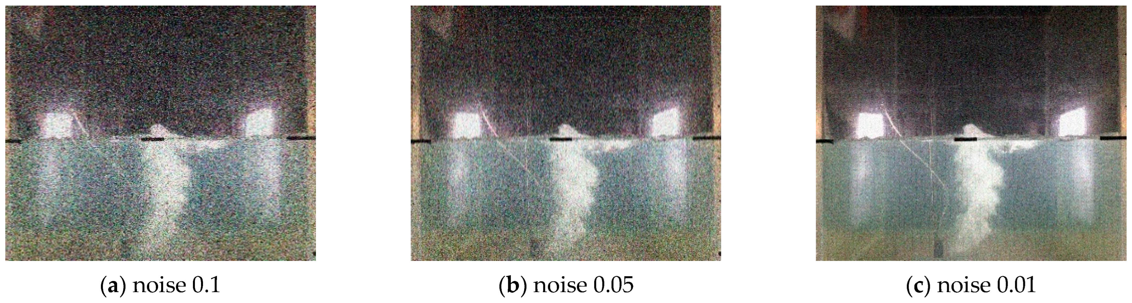
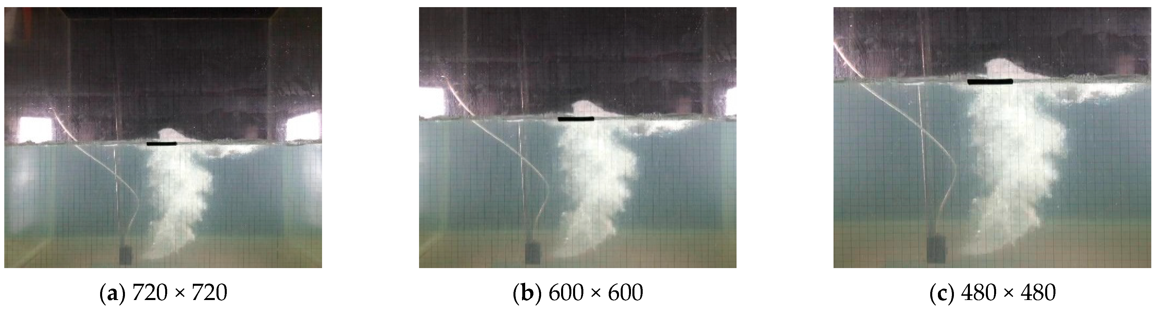
| Dataset | Annotation Files | Image Size | Noise | Source |
|---|---|---|---|---|
| Original datasets | xml files | 1280 × 720 | none | Experiment |
| Noise_0.1 | xml files | 1280 × 720 | 0.1 | Experiment |
| Noise_0.05 | xml files | 1280 × 720 | 0.05 | Experiment |
| Noise_0.01 | xml files | 1280 × 720 | 0.01 | Experiment |
| 720 × 720 | xml files | 720 × 720 | none | Experiment |
| 600 × 600 | xml files | 600 × 600 | none | Experiment |
| 480 × 480 | xml files | 480 × 480 | none | Experiment |
| Co. L. Mar. dataset | N/A | 320 × 240 | N/A | Real-world |
| BP dataset | N/A | 480 × 360 | N/A | Real-world |
| Configuration | Faster R-CNN Approach | YOLOv4 Approach |
|---|---|---|
| Pre-trained model | Faster_rcnn_inception_coco_v2 | YOLOv4.CONV.137 |
| Feature extractor | Inception V2 | CSPDarknet53 |
| Dataset structure | COCO | VOC2018 |
| Initial learning rate | 0.0002 | 0.001 |
| Batch size | 1 | 64 |
| Detection classes | 3 | 3 |
Disclaimer/Publisher’s Note: The statements, opinions and data contained in all publications are solely those of the individual author(s) and contributor(s) and not of MDPI and/or the editor(s). MDPI and/or the editor(s) disclaim responsibility for any injury to people or property resulting from any ideas, methods, instructions or products referred to in the content. |
© 2023 by the authors. Licensee MDPI, Basel, Switzerland. This article is an open access article distributed under the terms and conditions of the Creative Commons Attribution (CC BY) license (https://creativecommons.org/licenses/by/4.0/).
Share and Cite
Zhu, H.; Xie, W.; Li, J.; Shi, J.; Fu, M.; Qian, X.; Zhang, H.; Wang, K.; Chen, G. Advanced Computer Vision-Based Subsea Gas Leaks Monitoring: A Comparison of Two Approaches. Sensors 2023, 23, 2566. https://doi.org/10.3390/s23052566
Zhu H, Xie W, Li J, Shi J, Fu M, Qian X, Zhang H, Wang K, Chen G. Advanced Computer Vision-Based Subsea Gas Leaks Monitoring: A Comparison of Two Approaches. Sensors. 2023; 23(5):2566. https://doi.org/10.3390/s23052566
Chicago/Turabian StyleZhu, Hongwei, Weikang Xie, Junjie Li, Jihao Shi, Mingfu Fu, Xiaoyuan Qian, He Zhang, Kaikai Wang, and Guoming Chen. 2023. "Advanced Computer Vision-Based Subsea Gas Leaks Monitoring: A Comparison of Two Approaches" Sensors 23, no. 5: 2566. https://doi.org/10.3390/s23052566
APA StyleZhu, H., Xie, W., Li, J., Shi, J., Fu, M., Qian, X., Zhang, H., Wang, K., & Chen, G. (2023). Advanced Computer Vision-Based Subsea Gas Leaks Monitoring: A Comparison of Two Approaches. Sensors, 23(5), 2566. https://doi.org/10.3390/s23052566