
Comparing Direct Measurements and Three-Dimensional (3D) Scans for Evaluating Facial Soft Tissue
 , ,
, ,  , , and
Abstract
1. Introduction
- (1)
- Three dimensional (3D) facial scans are reproducible with high accuracy;
- (2)
- The actual and computed measurements are consistent and interchangeable.
2. Methodology
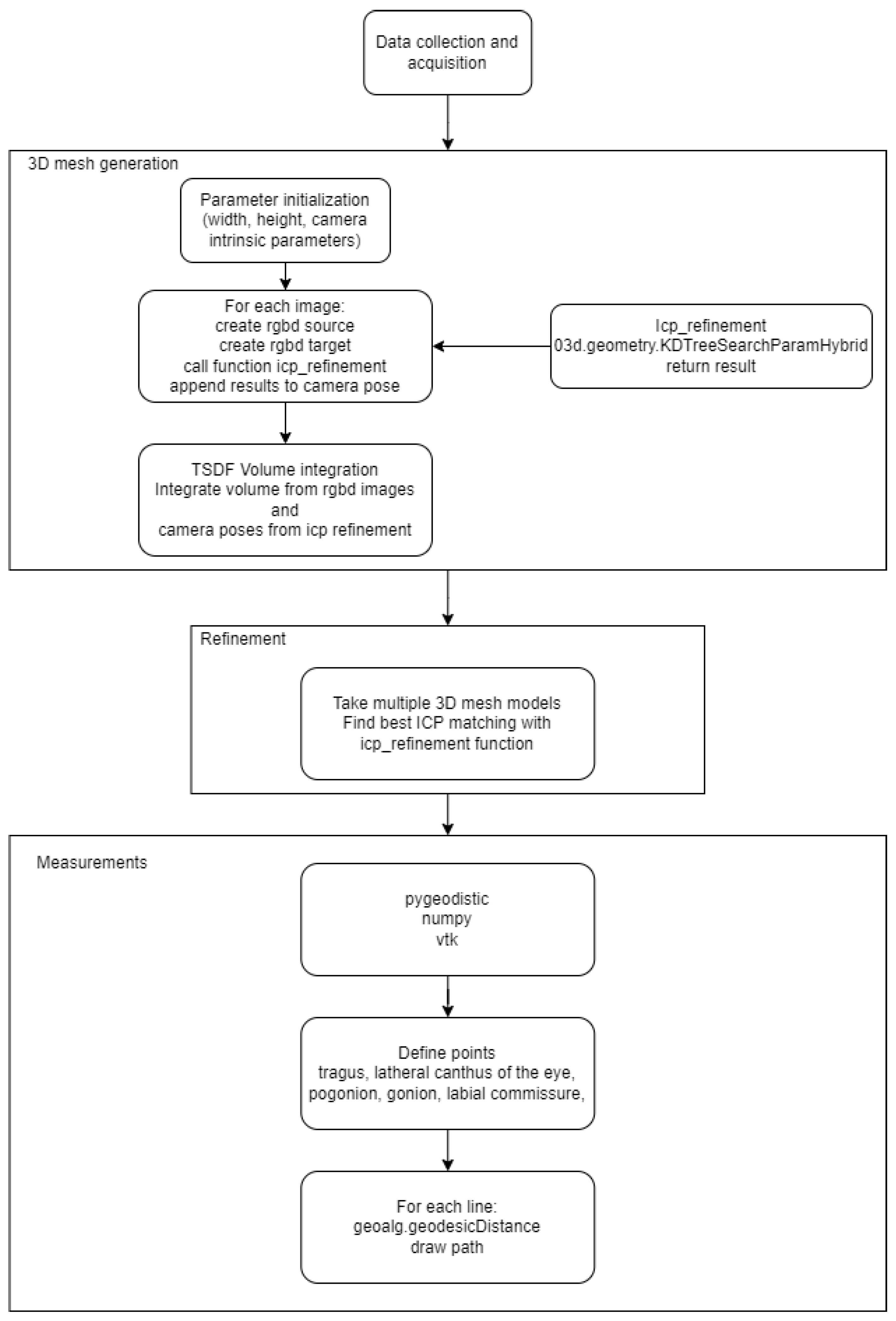
2.1. Data Acquisition and Analysis
2.2. Refinement
2.3. Mesh Metrics
2.3.1. Distance on 3D Mesh Model
2.3.2. Distance between 3D Meshes
3. Results
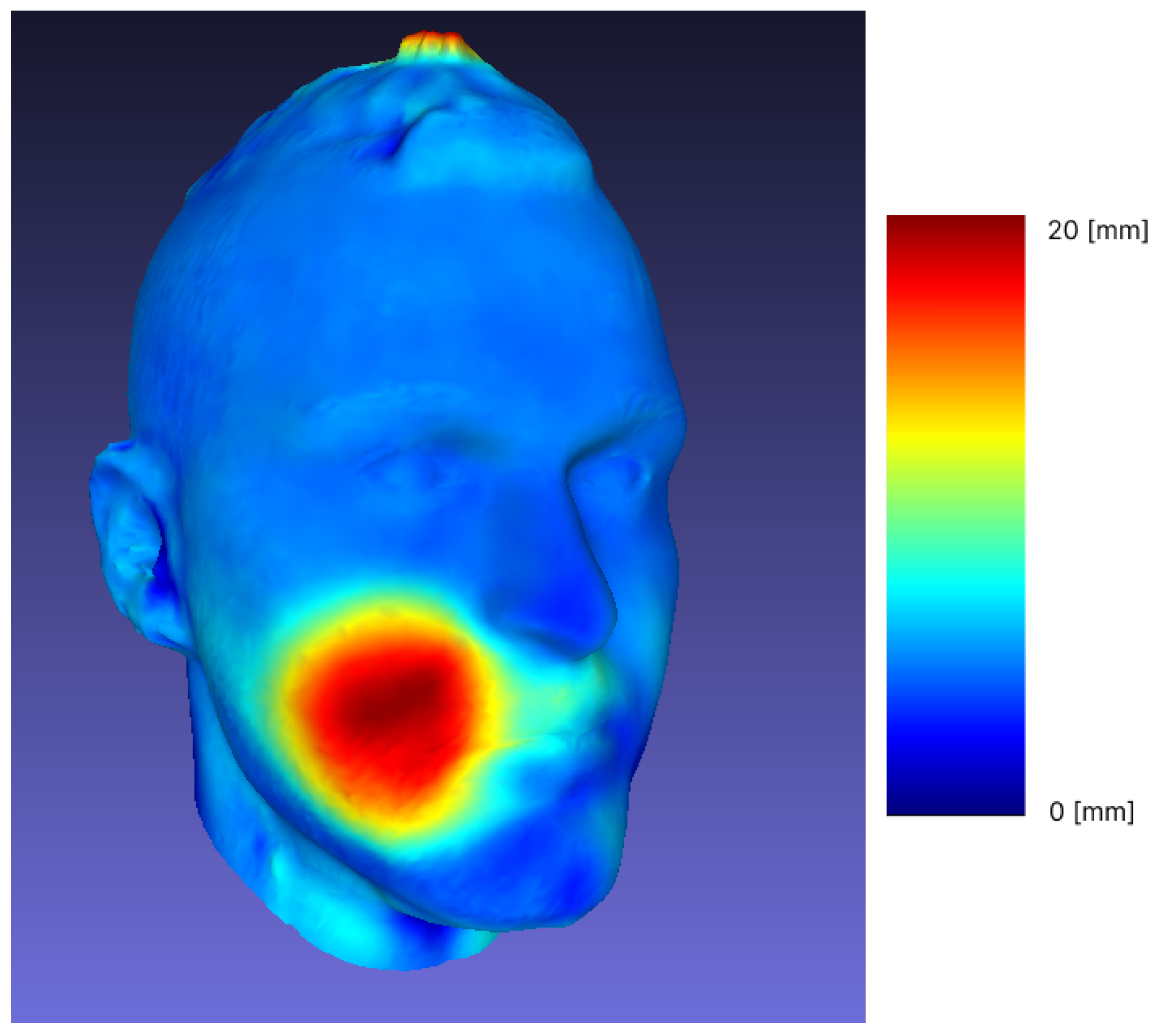
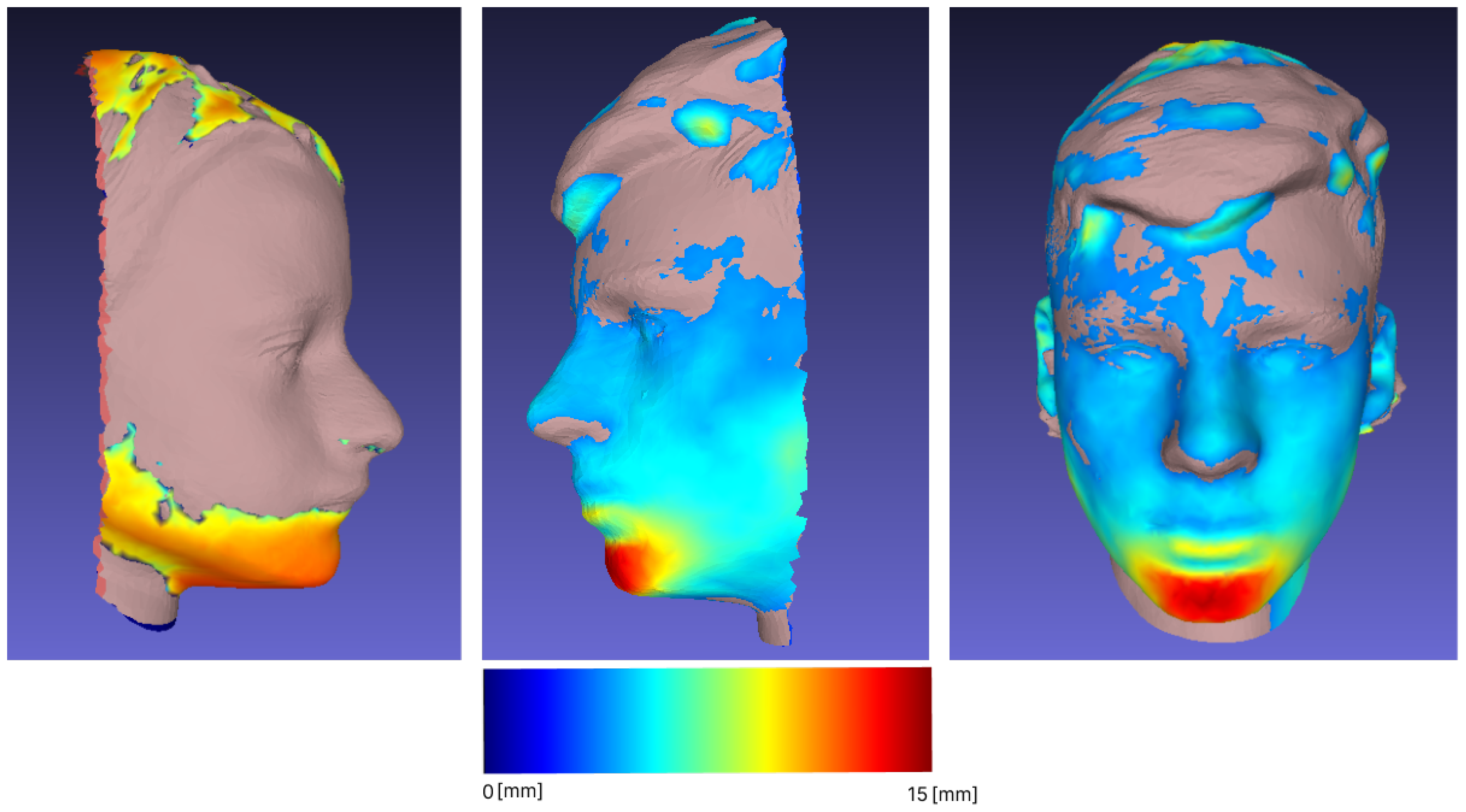
3.1. Reproducibility and Difference Visualization
3.2. Demarcation Lines Measurement
3.3. Forward Movement of the Mandible
4. Discussion
5. Conclusions
Author Contributions
Funding
Institutional Review Board Statement
Informed Consent Statement
Data Availability Statement
Acknowledgments
Conflicts of Interest
Abbreviations
| ICP | Iterative Closest Point |
| RMSE | Root mean square error |
| ICC | Intraclass correlation coefficient |
| FM | Fränkel manoeuvre |
| CT | Computed tomography |
| CBCT | Cone beam computed tomography |
Appendix A


References
- Chang, Y.J.; Ruellas, A.C.; Yatabe, M.S.; Westgate, P.M.; Cevidanes, L.H.; Huja, S.S. Soft Tissue Changes Measured WithThree-Dimensional Software ProvidesNew Insights for Surgical Predictions. J. Oral Maxillofac. Surg. 2017, 75, 2191–2201. [Google Scholar] [CrossRef]
- Bishara, S.E.; Cummins, D.M.; Jorgensen, G.J.; Jakobsen, J.R. A computer assisted photogrammetric analysis of softtissue changes after orthodontic treatment. Part I:Methodology and reliability. Am. J. Orthod. Dentofac. Orthop. 1995, 107, 633–639. [Google Scholar] [CrossRef] [PubMed]
- Baik, H.S.; Kim, S.Y. Facial soft-tissue changes in skeletal Class IIIorthognathic surgery patients analyzed with3-dimensional laser scanning. Am. J. Orthod. Dentofac. Orthop. 2010, 138, 167–178. [Google Scholar] [CrossRef]
- Atashi, M.H.A. Soft Tissue Esthetic Changes Following a Modified Twin Block Appliance Therapy: A Prospective Study. Int. J. Clin. Pediatr. Dent. 2020, 13, 255–260. [Google Scholar] [CrossRef]
- Ramos, E.U.; Bizelli, V.F.; Pereira Baggio, A.M.; Ferriolli, S.C.; Silva Prado, G.A.; Farnezi Bassi, A.P. Do the New Protocols of Platelet-Rich Fibrin Centrifugation Allow Better Control of Postoperative Complications and Healing After Surgery of Impacted Lower Third Molar? A Systematic Review and Meta-Analysis. J. Oral Maxillofac. Surg. Off. J. Am. Assoc. Oral Maxillofac. Surg. 2022, 80, 1238–1253. [Google Scholar] [CrossRef]
- Afat, İ.M.; Akdoğan, E.T.; Gönül, O. Effects of Leukocyte- and Platelet-Rich Fibrin Alone and Combined With Hyaluronic Acid on Pain, Edema, and Trismus After Surgical Extraction of Impacted Mandibular Third Molars. J. Oral Maxillofac. Surg. 2018, 76, 926–932. [Google Scholar] [CrossRef]
- Gulşen, U.; Şenturk, M.F. Effect of platelet rich fibrin on edema and pain following third molar surgery: A split mouth control study. BMC Oral Health 2017, 17, 79. [Google Scholar] [CrossRef]
- Rongo, R.; Bucci, R.; Adaimo, R.; Amato, M.; Martina, S.; Valletta, R.; D’anto, V. Two-dimensional versus three-dimensional Frankel Manoeuvre: A reproducibility study. Eur. J. Orthod. 2019, 42, 157–162. [Google Scholar] [CrossRef] [PubMed]
- Sattarzadeh, A.P.; Lee, R.T. Assessed facial normality after Twin Block therapy. Eur. J. Orthod. 2010, 32, 363–370. [Google Scholar] [CrossRef]
- Yıldırım, E.; Karaçay, Ş.; Tekin, D. Three-Dimensional Evaluation of Soft Tissue Changes after Functional Therapy. Scanning 2021, 2021, 9928101. [Google Scholar] [CrossRef]
- Farkas, L.G. Anthropometry of the Head and Face; Lippincott Williams & Wilkins: Philadelphia, PA, USA, 1994. [Google Scholar]
- Farnell, D.; Galloway, J.; Zhurov, A.; Richmond, S.; Perttiniemi, P.; Katić, V. Initial Results of Multilevel Principal Components Analysis of Facial Shape. In Medical Image Understanding and Analysis; Springer: Cham, Switzerland, 2017; pp. 674–685. [Google Scholar]
- Pellitteri, F.; Brucculeri, L.; Spedicato, G.A.; Siciliani, G.; Lombardo, L. Comparison of the accuracy of digital face scans obtained by two different scanners: An in vivo study. Angle Orthod. 2021, 91, 641–649. [Google Scholar] [CrossRef]
- Amezua, X.; Iturrate, M.; Garikano, X.; Solaberrieta, E. Analysis of the influence of the facial scanning method on the transfer accuracy of a maxillary digital scan to a 3D face scan for a virtual facebow technique: An in vitro study. J. Prosthet. Dent. 2022, 128, 1024–1031. [Google Scholar] [CrossRef]
- Gibelli, D.; Pucciarelli, V.; Poppa, P.; Cummaudo, M.; Dolci, C.; Cattaneo, C.; Sforza, C. Three-dimensional facial anatomy evaluation: Reliability of laser scanner consecutive scans procedure in comparison with stereophotogrammetry. J. Cranio-Maxillofac. Surg. 2018, 46, 1807–1813. [Google Scholar] [CrossRef]
- Curless, B.; Levoy, M. A volumetric method for building complex models from range images. In Proceedings of the 23rd Annual Conference on Computer Graphics and Interactive Techniques-SIGGRAPH ’96, New Orleans, LA, USA, 4–9 August 1996; ACM Press: New York, NY, USA, 1996. [Google Scholar] [CrossRef]
- Hruda, L.; Dvořák, J.; Váša, L. On evaluating consensus in RANSAC surface registration. Comput. Graph. Forum 2019, 38, 175–186. [Google Scholar] [CrossRef]
- Shi, X.; Peng, J.; Li, J.; Yan, P.; Gong, H. The Iterative Closest Point Registration Algorithm Based on the Normal Distribution Transformation. Procedia Comput. Sci. 2019, 147, 181–190. [Google Scholar] [CrossRef]
- Garland, M.; Heckbert, P.S. Surface simplification using quadric error metrics. In Proceedings of the 24th Annual Conference on Computer Graphics and Interactive Techniques—SIGGRAPH ’97, Los Angeles, CA, USA, 3–8 August 1997; ACM Press: New York, NY, USA, 1997. [Google Scholar] [CrossRef]
- Mitchell, J.S.B.; Mount, D.M.; Papadimitriou, C.H. The Discrete Geodesic Problem. SIAM J. Comput. 1987, 16, 647–668. [Google Scholar] [CrossRef]
- Newcombe, R.A.; Fitzgibbon, A.; Izadi, S.; Hilliges, O.; Molyneaux, D.; Kim, D.; Davison, A.J.; Kohi, P.; Shotton, J.; Hodges, S. KinectFusion: Real-time dense surface mapping and tracking. In Proceedings of the 2011 10th IEEE International Symposium on Mixed and Augmented Reality, Basel, Switzerland, 26–29 October 2011. [Google Scholar] [CrossRef]
- Kaplan, V.; Ciğerim, L.; Ciğerim, S.Ç.; Bazyel, Z.D.; Dinç, G. Comparison of Various Measurement Methods in the Evaluation of Swelling After Third Molar Surgery. Van Med. J. 2021, 28, 412–420. [Google Scholar] [CrossRef]
- Bland, J.M.; Altman, D. Statistical methods for assessing agreement between two methods of clinical measurement. Lancet 1986, 327, 307–310. [Google Scholar] [CrossRef]
- Koo, T.K.; Li, M.Y. A Guideline of Selecting and Reporting Intraclass Correlation Coefficients for Reliability Research. J. Chiropr. Med. 2016, 15, 155–163. [Google Scholar] [CrossRef]
- Besl, P.; McKay, N.D. A method for registration of 3-D shapes. IEEE Trans. Pattern Anal. Mach. Intell. 1992, 14, 239–256. [Google Scholar] [CrossRef]
- Borrmann, D.; Elseberg, J.; Lingemann, K.; Nüchter, A.; Hertzberg, J. Globally consistent 3D mapping with scan matching. Robot. Auton. Syst. 2008, 56, 130–142. [Google Scholar] [CrossRef]
- Zhurov, A.; Richmond, S.; Kau, C.H.; Toma, A. Averaging Facial Images; Wiley: New York, NY, USA, 2013; pp. 126–144. [Google Scholar] [CrossRef]
- Dijkstra, E.W. A Note on Two Problems in Connexion with Graphs. In Edsger Wybe Dijkstra; ACM: New York, NY, USA, 2022; pp. 287–290. [Google Scholar] [CrossRef]
- Kirsanov, D. Exact Geodesic for Triangular Meshes. Available online: https://www.mathworks.com/matlabcentral/fileexchange/18168-exact-geodesic-for-triangular-meshes (accessed on 17 November 2022).
- Aspert, N.; Santa-Cruz, D.; Ebrahimi, T. MESH: Measuring errors between surfaces using the Hausdorff distance. In Proceedings of the IEEE International Conference on Multimedia and Expo, Lausanne, Switzerland, 26–29 August 2002; Volume 1, pp. 705–708. [Google Scholar] [CrossRef]
- Kaspar, D. Application of Directional Antennas in RF-Based Indoor Localization Systems. Master’s Thesis, Swiss Federal Institute of Technology Zurich, Zürich, Switzerland, 2005. [Google Scholar]
- Giavarina, D. Understanding Bland Altman analysis. Biochem. Medica 2015, 25, 141–151. [Google Scholar] [CrossRef]
- Gibelli, D.; Pucciarelli, V.; Cappella, A.; Dolci, C.; Sforza, C. Are Portable Stereophotogrammetric Devices Reliable in Facial Imaging? A Validation Study of VECTRA H1 Device. J. Oral Maxillofac. Surg. 2018, 76, 1772–1784. [Google Scholar] [CrossRef]
- Jamison, P.L.; Ward, R.E. Brief communication: Measurement size, precision, and reliability in craniofacial anthropometry: Bigger is better. Am. J. Phys. Anthropol. 1993, 90, 495–500. [Google Scholar] [CrossRef] [PubMed]
- de Menezes, M.; Rosati, R.; Allievi, C.; Sforza, C. A Photographic System for the Three-Dimensional Study of Facial Morphology. Angle Orthod. 2009, 79, 1070–1077. [Google Scholar] [CrossRef]
- Maal, T.; Verhamme, L.; van Loon, B.; Plooij, J.; Rangel, F.; Kho, A.; Bronkhorst, E.; Bergé, S. Variation of the face in rest using 3D stereophotogrammetry. Int. J. Oral Maxillofac. Surg. 2011, 40, 1252–1257. [Google Scholar] [CrossRef]
- Kaplan, V.; Eroğlu, C.N. Comparison of the Effects of Daily Single-Dose Use of Flurbiprofen, Diclofenac Sodium, and Tenoxicam on Postoperative Pain, Swelling, and Trismus: A Randomized Double-Blind Study. J. Oral Maxillofac. Surg. 2016, 74, 1946.e1–1946.e6. [Google Scholar] [CrossRef]
- Jensen, E.; Palling, M. The gonial angle. Am. J. Orthod. 1954, 40, 120–133. [Google Scholar] [CrossRef]
- Martina, R.; D’Antò, V.; Chiodini, P.; Casillo, M.; Galeotti, A.; Tagliaferri, R.; Michelotti, A.; Cioffi, I. Reproducibility of the assessment of the Fränkel manoeuvre for the evaluation of sagittal skeletal discrepancies in Class II individuals. Eur. J. Orthod. 2015, 38, 409–413. [Google Scholar] [CrossRef]
- Fränkel, R.; Fränkel, C. Orofacial Orthopedics With the Function Regulator; S Karger Pub: Basel, Switzerland, 1989; p. 220. [Google Scholar]


| Line | Physical Distance [mm] | Computational Measurement [mm] | Diff [%] |
|---|---|---|---|
| tragus—lateral canthus of the eye (A) | 90.5 | 88.97 | −1.69 |
| tragus—pogonion (B) | 163 | 164.80 | +1.10 |
| gonion—lateral canthus of the eye (C) | 117 | 110.46 | −5.59 |
| gonion—labial commissure (D) | 97 | 92.85 | −4.27 |
| Line | ICC | |
|---|---|---|
| Left | Right | |
| tragus—lateral canthus of the eye (A) | −0.027 | 0.435 |
| tragus—pogonion (B) | 0.911 | 0.906 |
| gonion—lateral canthus of the eye (C) | 0.423 | 0.796 |
| gonion—labial commissure (D) | −0.196 | 0.766 |
| Line | Left | Right | ||||
|---|---|---|---|---|---|---|
| Diff | Mean [mm] | SD | Diff | Mean [mm] | SD | |
| tragus—lateral canthus of the eye (A) | 2.11 [0.79–3.17] | 1.60 | 1.21 | 1.95 [0.41–3] | 1.23 | 1.29 |
| tragus—pogonion (B) | 2.24 [1.29–6.59] | 2.694 | 1.90 | 1.17 [0.07–2.64] | 0.693 | 1.31 |
| gonion—lateral canthus of the eye (C) | 4.44 [0.72–7.52] | 3.292 | 3.69 | 6.62 [6–10] | 7.427 | 2.08 |
| gonion—labial commissure (D) | 10.43 [4.78–15.19] | 8.633 | 5.25 | 9.60 [4.15–13] | 7.940 | 4.44 |
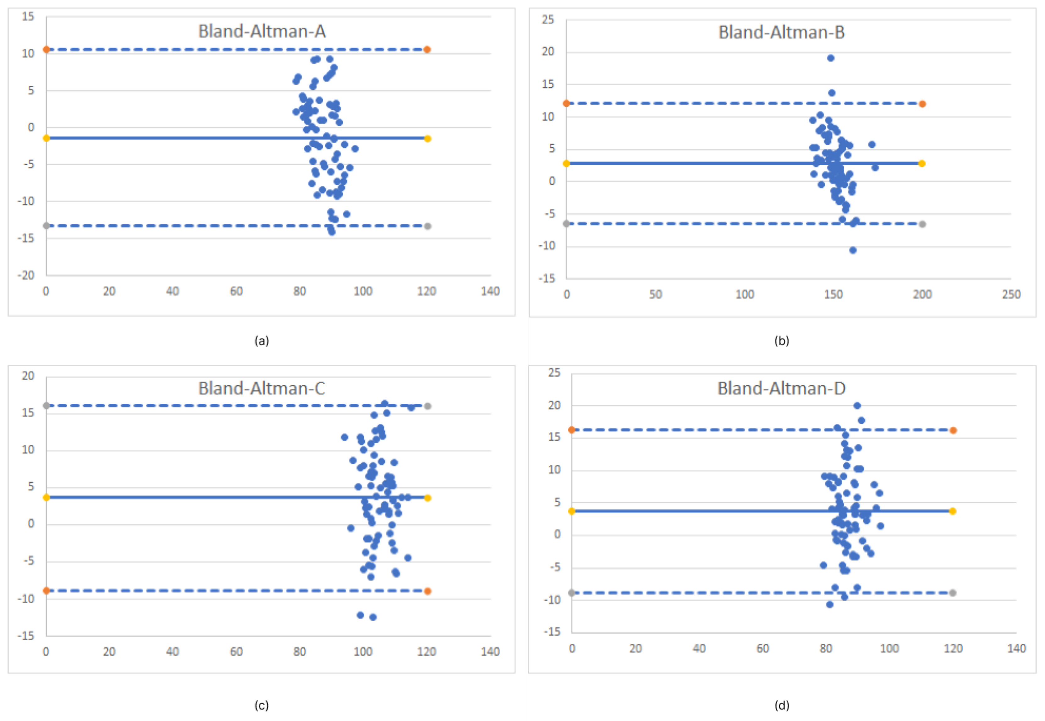
| Method Difference | Bias | SD of Bias | Min Limit (95%) | Max Limit (95%) |
|---|---|---|---|---|
| tr-eye (A) | −1.336 | 6.077 | −13.247 | 10.575 |
| tr-pog (B) | 2.752 | 4.746 | −6.551 | 12.055 |
| gon—eye (C) | 3.637 | 6.393 | −8.893 | 16.168 |
| gon—comm (D) | 3.779 | 6.391 | −8.746 | 16.305 |
| Sample | Min [mm] | Max [mm] | Mean [mm] | RMS |
|---|---|---|---|---|
| 1 | 0 | 19.59 | 1.04 | 1.86 |
| 2 | 0.000259 | 16.60 | 2.38 | 3.24 |
| 3 | 0.000038 | 10.32 | 1.39 | 2.08 |
| 4 | 0.000046 | 12.98 | 0.99 | 1.60 |
| 5 | 0.000015 | 21.80 | 1.91 | 3.26 |
| 6 | 0.000198 | 20.78 | 1.85 | 3.39 |
| 7 | 0 | 15.55 | 1.15 | 2.23 |
| 8 | 0.000031 | 25.98 | 2.98 | 4.77 |
| 9 | 0.000198 | 11.93 | 1.26 | 2.12 |
| 10 | 0.000153 | 27.86 | 2.33 | 4.39 |
Disclaimer/Publisher’s Note: The statements, opinions and data contained in all publications are solely those of the individual author(s) and contributor(s) and not of MDPI and/or the editor(s). MDPI and/or the editor(s) disclaim responsibility for any injury to people or property resulting from any ideas, methods, instructions or products referred to in the content. |
© 2023 by the authors. Licensee MDPI, Basel, Switzerland. This article is an open access article distributed under the terms and conditions of the Creative Commons Attribution (CC BY) license (https://creativecommons.org/licenses/by/4.0/).
Share and Cite
Gašparović, B.; Morelato, L.; Lenac, K.; Mauša, G.; Zhurov, A.; Katić, V. Comparing Direct Measurements and Three-Dimensional (3D) Scans for Evaluating Facial Soft Tissue. Sensors 2023, 23, 2412. https://doi.org/10.3390/s23052412
Gašparović B, Morelato L, Lenac K, Mauša G, Zhurov A, Katić V. Comparing Direct Measurements and Three-Dimensional (3D) Scans for Evaluating Facial Soft Tissue. Sensors. 2023; 23(5):2412. https://doi.org/10.3390/s23052412
Chicago/Turabian StyleGašparović, Boris, Luka Morelato, Kristijan Lenac, Goran Mauša, Alexei Zhurov, and Višnja Katić. 2023. "Comparing Direct Measurements and Three-Dimensional (3D) Scans for Evaluating Facial Soft Tissue" Sensors 23, no. 5: 2412. https://doi.org/10.3390/s23052412
APA StyleGašparović, B., Morelato, L., Lenac, K., Mauša, G., Zhurov, A., & Katić, V. (2023). Comparing Direct Measurements and Three-Dimensional (3D) Scans for Evaluating Facial Soft Tissue. Sensors, 23(5), 2412. https://doi.org/10.3390/s23052412