


Lossless Reconstruction of Convolutional Neural Network for Channel-Based Network Pruning


Abstract
:1. Introduction
- We propose a lossless reconstruction method using a residual block, skip connection, and batch normalization layers after the pruning algorithm to remove redundant channels.
- We show that compressing a large model leads to better performance than compressing a well-designed small network.
- We demonstrate that our method is able to significantly reduce runtime by measuring the latency on Raspberry Pi and Jetson Nano.
2. Related Works
2.1. Architecture Search
2.2. Unstructured Pruning
2.3. Structured Pruning
3. Methods
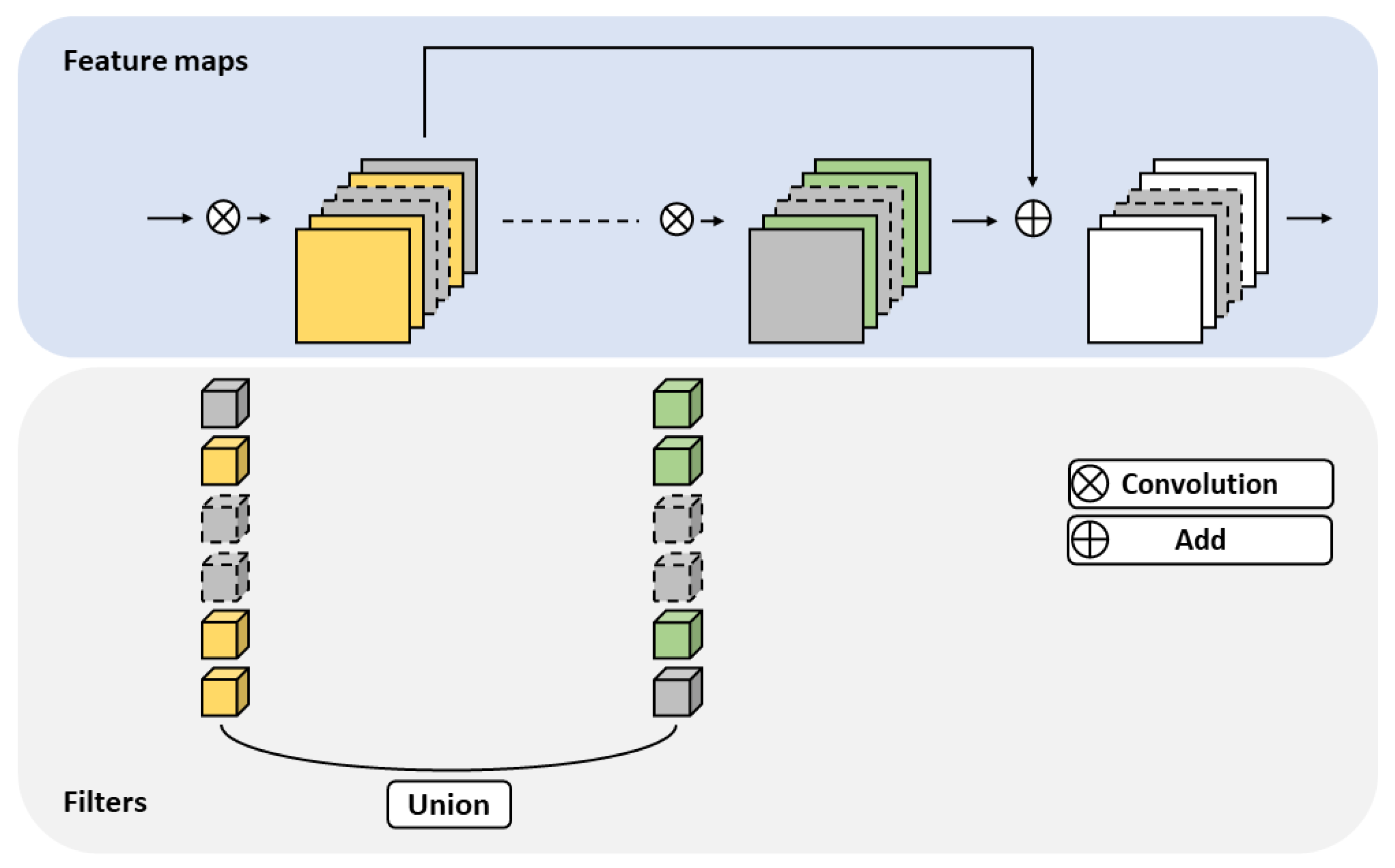
3.1. Residual Block
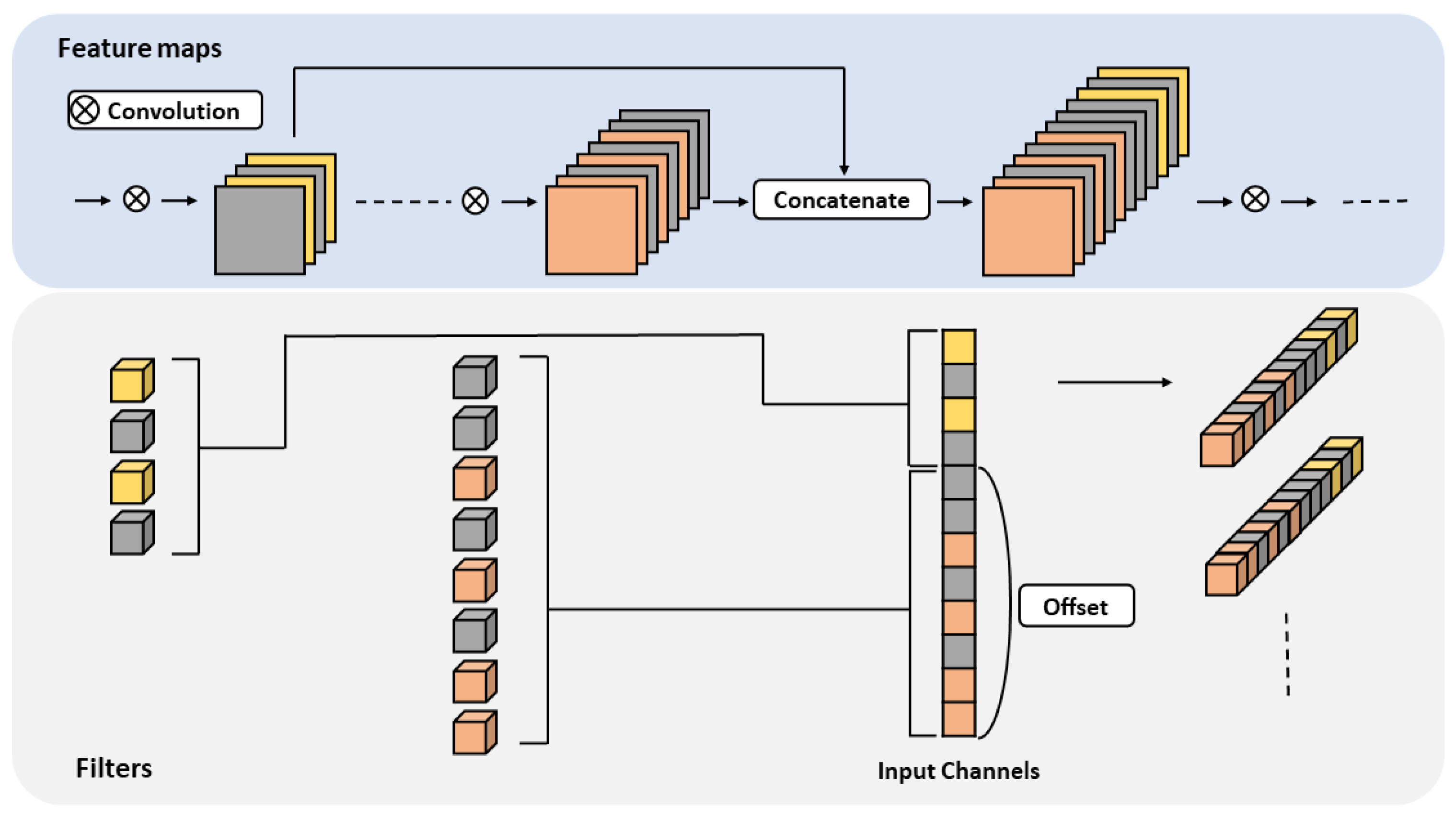
3.2. Skip Connection
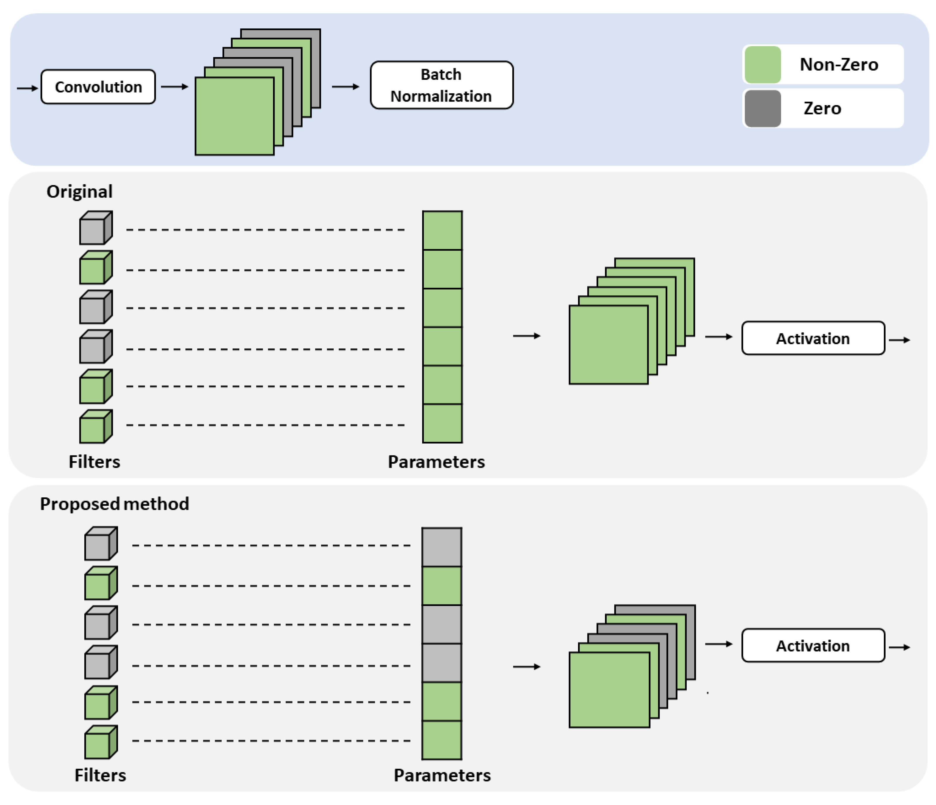
3.3. Batch Normalization
4. Experiments
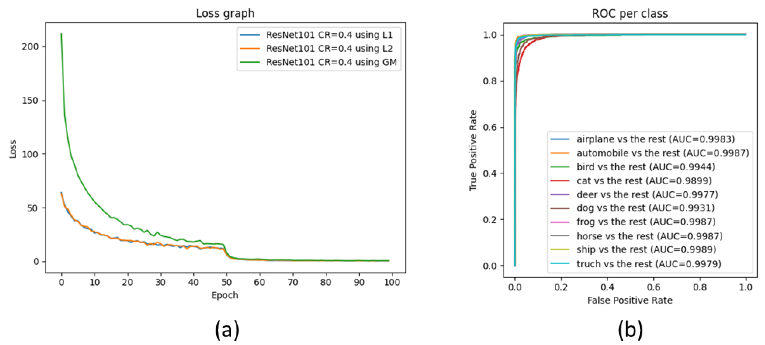
4.1. Image Classification
4.2. Semantic Segmentation
4.3. Object Detection
4.4. Latency
4.5. Ablation Study
4.5.1. Applying Union Operation in Residual Block
4.5.2. Influence of Pruning Batch Normalization Layer
4.5.3. Influence of Compression Process
5. Discussion
5.1. Strengths
5.2. Weaknesses and Limitations
6. Conclusions
Author Contributions
Funding
Institutional Review Board Statement
Informed Consent Statement
Data Availability Statement
Conflicts of Interest
References
- Simonyan, K.; Zisserman, A. Very deep convolutional networks for large-scale image recognition. arXiv 2014, arXiv:1409.1556. [Google Scholar]
- He, K.; Zhang, X.; Ren, S.; Sun, J. Deep residual learning for image recognition. In Proceedings of the IEEE Conference on Computer Vision and Pattern Recognition, Las Vegas, NV, USA, 27–30 June 2016; pp. 770–778. [Google Scholar]
- Dai, Z.; Liu, H.; Le, Q.V.; Tan, M. Coatnet: Marrying convolution and attention for all data sizes. Adv. Neural Inf. Process. Syst. 2021, 34, 3965–3977. [Google Scholar]
- Girshick, R. Fast r-cnn. In Proceedings of the IEEE International Conference on Computer Vision, Santiago, Chile, 7–13 December 2015; pp. 1440–1448. [Google Scholar]
- Liu, W.; Anguelov, D.; Erhan, D.; Szegedy, C.; Reed, S.; Fu, C.Y.; Berg, A.C. SSD: Single shot multibox detector. In Proceedings of the European Conference on Computer Vision, Amsterdam, The Netherlands, 11–14 October 2016; Springer: Berlin/Heidelberg, Germany, 2016; pp. 21–37. [Google Scholar]
- Redmon, J.; Divvala, S.; Girshick, R.; Farhadi, A. You only look once: Unified, real-time object detection. In Proceedings of the IEEE Conference on Computer Vision and Pattern Recognition, Las Vegas, NV, USA, 27–30 June 2016; pp. 779–788. [Google Scholar]
- Feng, S.; Fan, Y.; Tang, Y.; Cheng, H.; Zhao, C.; Zhu, Y.; Cheng, C. A Change Detection Method Based on Multi-Scale Adaptive Convolution Kernel Network and Multimodal Conditional Random Field for Multi-Temporal Multispectral Images. Remote Sens. 2022, 14, 5368. [Google Scholar] [CrossRef]
- Zhang, H.; Li, F.; Liu, S.; Zhang, L.; Su, H.; Zhu, J.; Ni, L.M.; Shum, H.Y. Dino: Detr with improved denoising anchor boxes for end-to-end object detection. arXiv 2022, arXiv:2203.03605. [Google Scholar]
- Badrinarayanan, V.; Kendall, A.; Cipolla, R. Segnet: A deep convolutional encoder-decoder architecture for image segmentation. IEEE Trans. Pattern Anal. Mach. Intell. 2017, 39, 2481–2495. [Google Scholar] [CrossRef] [PubMed]
- Ronneberger, O.; Fischer, P.; Brox, T. U-net: Convolutional networks for biomedical image segmentation. In Proceedings of the International Conference on Medical Image Computing and Computer-Assisted Intervention, Munich, Germany, 5–9 October 2015; Springer: Berlin/Heidelberg, Germany, 2015; pp. 234–241. [Google Scholar]
- Paszke, A.; Chaurasia, A.; Kim, S.; Culurciello, E. Enet: A deep neural network architecture for real-time semantic segmentation. arXiv 2016, arXiv:1606.02147. [Google Scholar]
- Saini, V.K.; Kumar, R.; Mathur, A.; Saxena, A. Short term forecasting based on hourly wind speed data using deep learning algorithms. In Proceedings of the 2020 3rd International Conference on Emerging Technologies in Computer Engineering: Machine Learning and Internet of Things (ICETCE), Jaipur, India, 7–8 February 2020; pp. 1–6. [Google Scholar]
- Han, S.; Pool, J.; Tran, J.; Dally, W. Learning both weights and connections for efficient neural network. In Proceedings of the Advances in Neural Information Processing Systems, Montreal, QC, Canada, 7–12 December 2015; Volume 28. [Google Scholar]
- Han, S.; Mao, H.; Dally, W.J. Deep compression: Compressing deep neural networks with pruning, trained quantization and huffman coding. In Proceedings of the International Conference on Learning Representations, San Diego, CA, USA, 7–9 May 2015. [Google Scholar]
- Dong, X.; Chen, S.; Pan, S. Learning to prune deep neural networks via layer-wise optimal brain surgeon. In Proceedings of the Advances in Neural Information Processing Systems, Long Beach, CA, USA, 4–9 December 2017; Volume 30. [Google Scholar]
- Xiao, X.; Wang, Z.; Rajasekaran, S. Autoprune: Automatic network pruning by regularizing auxiliary parameters. In Proceedings of the 33rd Conference on Neural Information Processing Systems (NeurIPS 2019), Vancouver, CA, USA, 8–14 December 2019; Volume 32. [Google Scholar]
- Li, H.; Kadav, A.; Durdanovic, I.; Samet, H.; Graf, H.P. Pruning filters for efficient convnets. arXiv 2016, arXiv:1608.08710. [Google Scholar]
- Ye, J.; Lu, X.; Lin, Z.; Wang, J.Z. Rethinking the smaller-norm-less-informative assumption in channel pruning of convolution layers. In Proceedings of the International Conference on Learning Representations, Vancouver, BC, Canada, 30 April–3 May 2018. [Google Scholar]
- He, Y.; Liu, P.; Wang, Z.; Hu, Z.; Yang, Y. Filter pruning via geometric median for deep convolutional neural networks acceleration. In Proceedings of the IEEE/CVF Conference on Computer Vision and Pattern Recognition, Long Beach, CA, USA, 15–20 June 2019; pp. 4340–4349. [Google Scholar]
- Liu, Z.; Mu, H.; Zhang, X.; Guo, Z.; Yang, X.; Cheng, K.T.; Sun, J. Metapruning: Meta learning for automatic neural network channel pruning. In Proceedings of the IEEE/CVF International Conference on Computer Vision, Seoul, Republic of Korea, 27 October–2 November 2019; pp. 3296–3305. [Google Scholar]
- Chin, T.W.; Ding, R.; Zhang, C.; Marculescu, D. Towards efficient model compression via learned global ranking. In Proceedings of the IEEE/CVF Conference on Computer Vision and Pattern Recognition, Seattle, WA, USA, 13–19 June 2020; pp. 1518–1528. [Google Scholar]
- Gao, S.; Huang, F.; Cai, W.; Huang, H. Network pruning via performance maximization. In Proceedings of the IEEE/CVF Conference on Computer Vision and Pattern Recognition, Nashville, TN, USA, 19–25 June 2021; pp. 9270–9280. [Google Scholar]
- Tan, M.; Le, Q. Efficientnet: Rethinking model scaling for convolutional neural networks. In Proceedings of the International Conference on Machine Learning, PMLR, Long Beach, CA, USA, 9–15 June 2019; pp. 6105–6114. [Google Scholar]
- Zamir, S.W.; Arora, A.; Khan, S.; Hayat, M.; Khan, F.S.; Yang, M.H.; Shao, L. Multi-Stage Progressive Image Restoration. In Proceedings of the CVPR, Online, 19–25 June 2021. [Google Scholar]
- Liu, Z.; Mao, H.; Wu, C.Y.; Feichtenhofer, C.; Darrell, T.; Xie, S. A convnet for the 2020s. In Proceedings of the IEEE/CVF Conference on Computer Vision and Pattern Recognition, New Orleans, LA, USA, 18–24 June 2022; pp. 11976–11986. [Google Scholar]
- Howard, A.G.; Zhu, M.; Chen, B.; Kalenichenko, D.; Wang, W.; Weyand, T.; Andreetto, M.; Adam, H. Mobilenets: Efficient convolutional neural networks for mobile vision applications. arXiv 2017, arXiv:1704.04861. [Google Scholar]
- Zoph, B.; Le, Q.V. Neural architecture search with reinforcement learning. In Proceedings of the International Conference on Learning Representations, Toulon, France, 24–26 April 2017. [Google Scholar]
- Liu, H.; Simonyan, K.; Yang, Y. Darts: Differentiable architecture search. arXiv 2018, arXiv:1806.09055. [Google Scholar]
- Radosavovic, I.; Kosaraju, R.P.; Girshick, R.; He, K.; Dollár, P. Designing network design spaces. In Proceedings of the IEEE/CVF Conference on Computer Vision and Pattern Recognition, Seattle, WA, USA, 13–19 June 2020; pp. 10428–10436. [Google Scholar]
- LeCun, Y.; Denker, J.; Solla, S. Optimal brain damage. In Proceedings of the Advances in Neural Information Processing Systems, NIPS Conference, Denver, CO, USA, 27–30 November 1989; Volume 2. [Google Scholar]
- Hassibi, B.; Stork, D. Second order derivatives for network pruning: Optimal brain surgeon. In Proceedings of the Advances in Neural Information Processing Systems, Denver, CO, USA, 30 November–3 December 1992; Volume 5. [Google Scholar]
- Aghasi, A.; Abdi, A.; Nguyen, N.; Romberg, J. Net-trim: Convex pruning of deep neural networks with performance guarantee. In Proceedings of the Advances in Neural Information Processing Systems, Long Beach, CA, USA, 4–9 December 2017; Volume 30. [Google Scholar]
- Hu, H.; Peng, R.; Tai, Y.W.; Tang, C.K. Network trimming: A data-driven neuron pruning approach towards efficient deep architectures. arXiv 2016, arXiv:1607.03250. [Google Scholar]
- Molchanov, D.; Ashukha, A.; Vetrov, D. Variational dropout sparsifies deep neural networks. In Proceedings of the International Conference on Machine Learning, PMLR, Sydney, Australia, 6–11 August 2017; pp. 2498–2507. [Google Scholar]
- Lee, E.; Hwang, Y. Layer-Wise Network Compression Using Gaussian Mixture Model. Electronics 2021, 10, 72. [Google Scholar] [CrossRef]
- Yu, X.; Serra, T.; Ramalingam, S.; Zhe, S. The Combinatorial Brain Surgeon: Pruning Weights That Cancel One Another in Neural Networks. In Proceedings of the 39th International Conference on Machine Learning, Baltimore, MD, USA, 17–23 July 2022; Chaudhuri, K., Jegelka, S., Song, L., Szepesvari, C., Niu, G., Sabato, S., Eds.; Proceedings of Machine Learning Research. 2022; Volume 162, pp. 25668–25683. [Google Scholar]
- Wimmer, P.; Mehnert, J.; Condurache, A. Interspace Pruning: Using Adaptive Filter Representations To Improve Training of Sparse CNNs. In Proceedings of the IEEE/CVF Conference on Computer Vision and Pattern Recognition (CVPR), New Orleans, LA, USA, 18–24 June 2022; pp. 12527–12537. [Google Scholar]
- Luo, J.H.; Wu, J.; Lin, W. Thinet: A filter level pruning method for deep neural network compression. In Proceedings of the IEEE International Conference on Computer Vision, Venice, Italy, 22–29 October 2017; pp. 5058–5066. [Google Scholar]
- Yu, R.; Li, A.; Chen, C.F.; Lai, J.H.; Morariu, V.I.; Han, X.; Gao, M.; Lin, C.Y.; Davis, L.S. Nisp: Pruning networks using neuron importance score propagation. In Proceedings of the IEEE Conference on Computer Vision and Pattern Recognition, Salt Lake City, UT, USA, 18–23 June 2018; pp. 9194–9203. [Google Scholar]
- Li, Y.; Gu, S.; Zhang, K.; Van Gool, L.; Timofte, R. Dhp: Differentiable meta pruning via hypernetworks. In Proceedings of the European Conference on Computer Vision; Springer: Berlin/Heidelberg, Germany; Springer: Glasgow, UK, 2020; pp. 608–624. [Google Scholar]
- Li, Y.; Adamczewski, K.; Li, W.; Gu, S.; Timofte, R.; Van Gool, L. Revisiting Random Channel Pruning for Neural Network Compression. In Proceedings of the IEEE/CVF Conference on Computer Vision and Pattern Recognition, New Orleans, LA, USA, 18–24 June 2022; pp. 191–201. [Google Scholar]
- Shen, M.; Molchanov, P.; Yin, H.; Alvarez, J.M. When to prune? a policy towards early structural pruning. In Proceedings of the IEEE/CVF Conference on Computer Vision and Pattern Recognition, New Orleans, LA, USA, 18–24 June 2022; pp. 12247–12256. [Google Scholar]
- Hou, Z.; Qin, M.; Sun, F.; Ma, X.; Yuan, K.; Xu, Y.; Chen, Y.K.; Jin, R.; Xie, Y.; Kung, S.Y. CHEX: CHannel EXploration for CNN Model Compression. In Proceedings of the IEEE/CVF Conference on Computer Vision and Pattern Recognition (CVPR), New Orleans, LA, USA, 18–24 June 2022; pp. 12287–12298. [Google Scholar]
- Ioffe, S.; Szegedy, C. Batch normalization: Accelerating deep network training by reducing internal covariate shift. In Proceedings of the International conference on machine learning, PMLR, Lille, France, 7–9 July 2015; pp. 448–456. [Google Scholar]
- Krizhevsky, A.; Hinton, G. Learning Multiple Layers of Features from Tiny Images; University of Toronto: Toronto, ON, Canada, 2009. [Google Scholar]
- Long, J.; Shelhamer, E.; Darrell, T. Fully convolutional networks for semantic segmentation. In Proceedings of the IEEE Conference on Computer Vision and Pattern Recognition, Boston, MA, USA, 7–12 June 2015; pp. 3431–3440. [Google Scholar]
- Everingham, M.; Eslami, S.; Van Gool, L.; Williams, C.K.; Winn, J.; Zisserman, A. The pascal visual object classes challenge: A retrospective. Int. J. Comput. Vis. 2015, 111, 98–136. [Google Scholar] [CrossRef]
- Redmon, J.; Farhadi, A. Yolov3: An incremental improvement. arXiv 2018, arXiv:1804.02767. [Google Scholar]
- Curtin, B.H.; Matthews, S.J. Deep learning for inexpensive image classification of wildlife on the Raspberry Pi. In Proceedings of the 2019 IEEE 10th Annual Ubiquitous Computing, Electronics & Mobile Communication Conference (UEMCON), New York, NY, USA, 10–12 October 2019; pp. 0082–0087. [Google Scholar]


| Image Classification | Semantic Segmentation | Object Detection | ||||
|---|---|---|---|---|---|---|
| Original Model | Pruned Model | Original Model | Pruned Model | Original Model | Pruned Model | |
| batch size | 128 | 128 | 16 | 16 | 16 | 16 |
| GPU | 2 | 2 | 1 | 1 | 1 | 1 |
| epoch | 200 | 100 | 100 | 50 | 150 | 100 |
| optimizer | SGD | SGD | SGD | SGD | SGD | SGD |
| momentum | 0.9 | 0.9 | 0.9 | 0.9 | 0.9 | 0.9 |
| weight decay | 0.0001 | 0.0001 | 0.0001 | 0.0001 | 0.0005 | 0.0005 |
| initial lr | 0.1 | 0.01 | 0.001 | 0.001 | 0.0001 | 0.0001 |
| lr scheduler | divided by 10 | divided by 5 | divided by 5 | divided by 5 | cosine annealing | cosine annealing |
| at 90, 140 epochs | at 50, 70 epochs | at 50, 70 epochs | at 25, 40 epochs | (0.0001∼0.00001) | (0.0001∼0.00001) | |
| Model | CR | Method | FLOPs(M) | Params(M) | Acc. (%) | Acc.↓ (%) |
|---|---|---|---|---|---|---|
| ResNet101- baseline | - | - | 1269.58 | 44.54 | 93.30 | 0.00 |
| ResNet101 | 0.4 | L1 | 621.86 | 21.86 | 93.26 | 0.04 |
| 0.4 | L2 | 621.78 | 21.89 | 93.20 | 0.10 | |
| 0.4 | GM | 633.40 | 23.39 | 93.06 | 0.24 | |
| ResNet50 | - | - | 661.00 | 25.54 | 92.67 | 0.63 |
| ResNet101 - baseline | - | - | 1269.58 | 44.54 | 93.30 | 0.00 |
| ResNet101 | 0.45 | L1 | 553.16 | 19.49 | 92.92 | 0.38 |
| 0.45 | L2 | 553.7 | 19.54 | 93.16 | 0.14 | |
| 0.45 | GM | 564.55 | 21.11 | 90.02 | 2.98 | |
| ResNet50 | - | - | 661.00 | 25.54 | 92.67 | 0.63 |
| ResNet50 | 0.1 | L1 | 571.66 | 22.17 | 93.15 | 0.15 |
| 0.1 | L2 | 571.62 | 22.16 | 93.11 | 0.19 | |
| 0.1 | GM | 573.54 | 22.45 | 93.11 | 0.19 | |
| ResNet34 | - | - | 585.31 | 21.78 | 92.47 | 0.83 |
| ResNet101 - baseline | - | - | 1269.58 | 44.54 | 93.30 | 0.00 |
| ResNet101 | 0.7 | L1 | 257.7 | 9.20 | 92.30 | 1.00 |
| 0.7 | L2 | 259.7 | 9.24 | 92.47 | 0.83 | |
| 0.7 | GM | 264.3 | 10.76 | 89.92 | 3.38 | |
| ResNet50 | 0.5 | L1 | 267.48 | 10.48 | 92.61 | 0.69 |
| 0.5 | L2 | 269.02 | 10.47 | 92.70 | 0.60 | |
| 0.5 | GM | 275.22 | 11.88 | 92.52 | 0.78 | |
| ResNet34 | - | - | 585.31 | 21.78 | 92.47 | 0.83 |
| ResNet34 | 0.5 | L1 | 281.42 | 10.33 | 92.13 | 1.17 |
| 0.5 | L2 | 280.86 | 10.23 | 91.72 | 1.58 | |
| 0.5 | GM | 286.12 | 10.73 | 91.14 | 2.16 | |
| ResNet18 | - | - | 282.71 | 11.68 | 90.77 | 2.53 |
| Model | CR | Method | FLOPs(G) | Params(M) | ↓ | mIoU | mIoU ↓ | |
|---|---|---|---|---|---|---|---|---|
| FCN_ResNet101 - baseline | - | - | 397.86 | 54.31 | 94.87 | 0.00 | 75.1 | 0.00 |
| FCN_ResNet101 | 0.3 | L1 | 260.4 | 35.57 | 94.12 | 0.75 | 72.8 | 2.3 |
| 0.3 | L2 | 260.72 | 35.61 | 94.23 | 0.64 | 73.2 | 1.9 | |
| 0.3 | GM | 276.42 | 37.78 | 92.69 | 2.18 | 66.6 | 8.5 | |
| FCN_ResNet50 | - | - | 260.93 | 35.32 | 93.66 | 1.21 | 71.0 | 4.1 |
| Model | CR | Method | FLOPs (G) | Params (M) | mAP | mAP ↓ |
|---|---|---|---|---|---|---|
| YOLOv3 - baseline | - | - | 65.658 | 61.626 | 0.545 | 0.000 |
| YOLOv3 | 0.9 | L1 | 3.229 | 2.455 | 0.421 | 0.124 |
| 0.9 | L2 | 3.252 | 2.485 | 0.424 | 0.121 | |
| 0.9 | GM | 3.248 | 2.484 | 0.423 | 0.122 | |
| YOLOv3-tiny | - | - | 5.518 | 8.714 | 0.370 | 0.175 |
| Device | Model | CR | mAP | FLOPs (G) | Latency (s) |
|---|---|---|---|---|---|
| Raspberry Pi 4 8GB | YOLOv3 | - | 0.545 | 65.658 | 5.0755 |
| 0.5 | 0.543 | 14.671 | 1.5771 | ||
| 0.7 | 0.536 | 10.019 | 1.1880 | ||
| 0.9 | 0.423 | 3.248 | 0.6227 | ||
| YOLOv3-tiny | - | 0.370 | 5.518 | 0.6024 | |
| Jetson Nano B01 4GB | YOLOv3 | - | 0.545 | 65.658 | 0.5347 |
| 0.5 | 0.543 | 14.671 | 0.1647 | ||
| 0.7 | 0.538 | 10.019 | 0.1236 | ||
| 0.9 | 0.423 | 3.248 | 0.1009 | ||
| YOLOv3-tiny | - | 0.370 | 5.518 | 0.0821 | |
| RTX 2080 Ti | YOLOv3 | - | 0.545 | 65.658 | 0.0076 |
| 0.5 | 0.543 | 14.671 | 0.0030 | ||
| 0.7 | 0.538 | 10.019 | 0.0024 | ||
| 0.9 | 0.423 | 3.248 | 0.0016 | ||
| YOLOv3-tiny | - | 0.370 | 5.518 | 0.0013 |
| Model | Method | FLOPs Ratio (%) | Top-1 Error (%) | Latency (ms) | |
|---|---|---|---|---|---|
| Before Reconstruction | After Reconstruction | ||||
| ResNet50 | L1 | 40.27 | 7.33 → 7.39 (+0.06) | 8.647 | 5.467 |
| L2 | 40.50 | 7.33 → 7.30 (−0.03) | 5.484 | ||
| GM | 41.31 | 7.33 → 7.48 (+0.15) | 5.676 | ||
| DHP-38 [40] | 39.07 | 7.05 → 7.06 (+0.01) | 5.333 | ||
| Model | Method | CR | Operation | Finetune Acc | Reconstruction Acc | Acc Loss |
|---|---|---|---|---|---|---|
| ResNet50 | L1 | 0.5 | AND | 92.82% | 10.02% | 82.80% |
| L1 | 0.5 | OR | 92.82% | 92.82% | 0.00% | |
| L2 | 0.5 | AND | 92.70% | 10.02% | 82.68% | |
| L2 | 0.5 | OR | 92.70% | 92.70% | 0.00% | |
| GM | 0.5 | AND | 92.80% | 9.99% | 82.81% | |
| GM | 0.5 | OR | 92.80% | 92.80% | 0.00% |
| Model | Method | CR | Batch norm. | Finetune Acc | Reconstruction Acc | Acc Loss |
|---|---|---|---|---|---|---|
| ResNet50 | L1 | 0.5 | ✓ | 92.53% | 92.53% | 0.00% |
| L1 | 0.5 | 92.45% | 89.32% | 3.13% | ||
| L2 | 0.5 | ✓ | 92.72% | 92.72% | 0.00% | |
| L2 | 0.5 | 92.71% | 88.27% | 4.44% | ||
| GM | 0.5 | ✓ | 92.42% | 92.42% | 0.00% | |
| GM | 0.5 | 92.51% | 55.17% | 37.34% |
Disclaimer/Publisher’s Note: The statements, opinions and data contained in all publications are solely those of the individual author(s) and contributor(s) and not of MDPI and/or the editor(s). MDPI and/or the editor(s) disclaim responsibility for any injury to people or property resulting from any ideas, methods, instructions or products referred to in the content. |
© 2023 by the authors. Licensee MDPI, Basel, Switzerland. This article is an open access article distributed under the terms and conditions of the Creative Commons Attribution (CC BY) license (https://creativecommons.org/licenses/by/4.0/).
Share and Cite
Lee, D.; Lee, E.; Hwang, Y. Lossless Reconstruction of Convolutional Neural Network for Channel-Based Network Pruning. Sensors 2023, 23, 2102. https://doi.org/10.3390/s23042102
Lee D, Lee E, Hwang Y. Lossless Reconstruction of Convolutional Neural Network for Channel-Based Network Pruning. Sensors. 2023; 23(4):2102. https://doi.org/10.3390/s23042102
Chicago/Turabian StyleLee, Donghyeon, Eunho Lee, and Youngbae Hwang. 2023. "Lossless Reconstruction of Convolutional Neural Network for Channel-Based Network Pruning" Sensors 23, no. 4: 2102. https://doi.org/10.3390/s23042102
APA StyleLee, D., Lee, E., & Hwang, Y. (2023). Lossless Reconstruction of Convolutional Neural Network for Channel-Based Network Pruning. Sensors, 23(4), 2102. https://doi.org/10.3390/s23042102