
Multitier Web System Reliability: Identifying Causative Metrics and Analyzing Performance Anomaly Using a Regression Model


Abstract
:1. Introduction
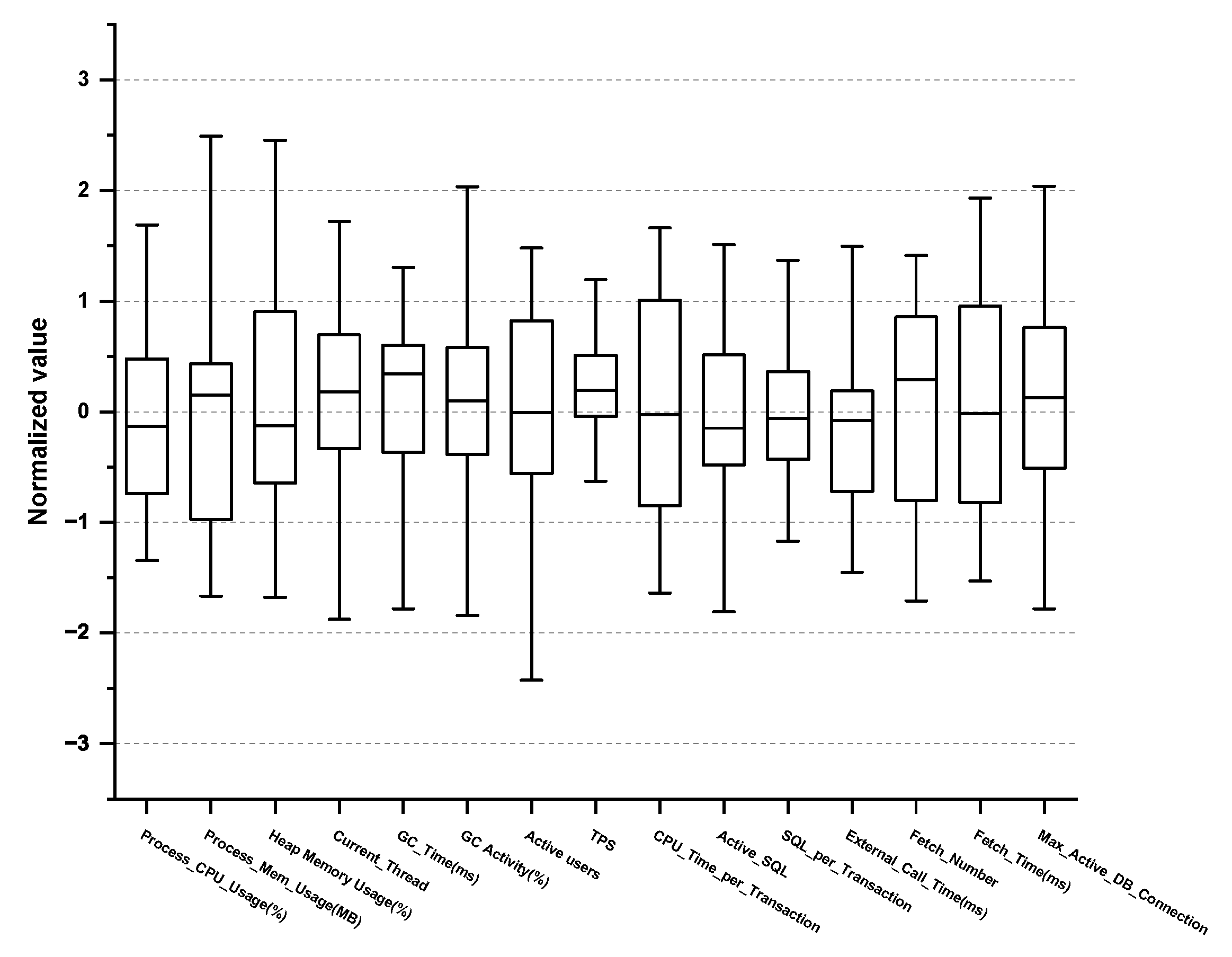
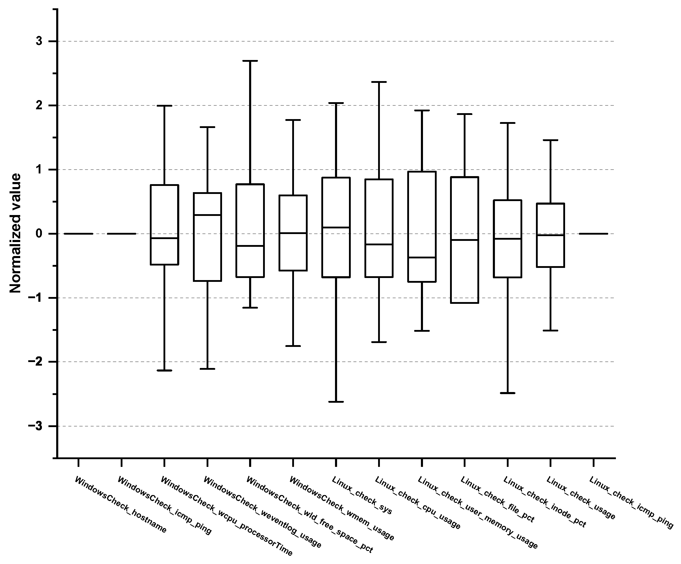
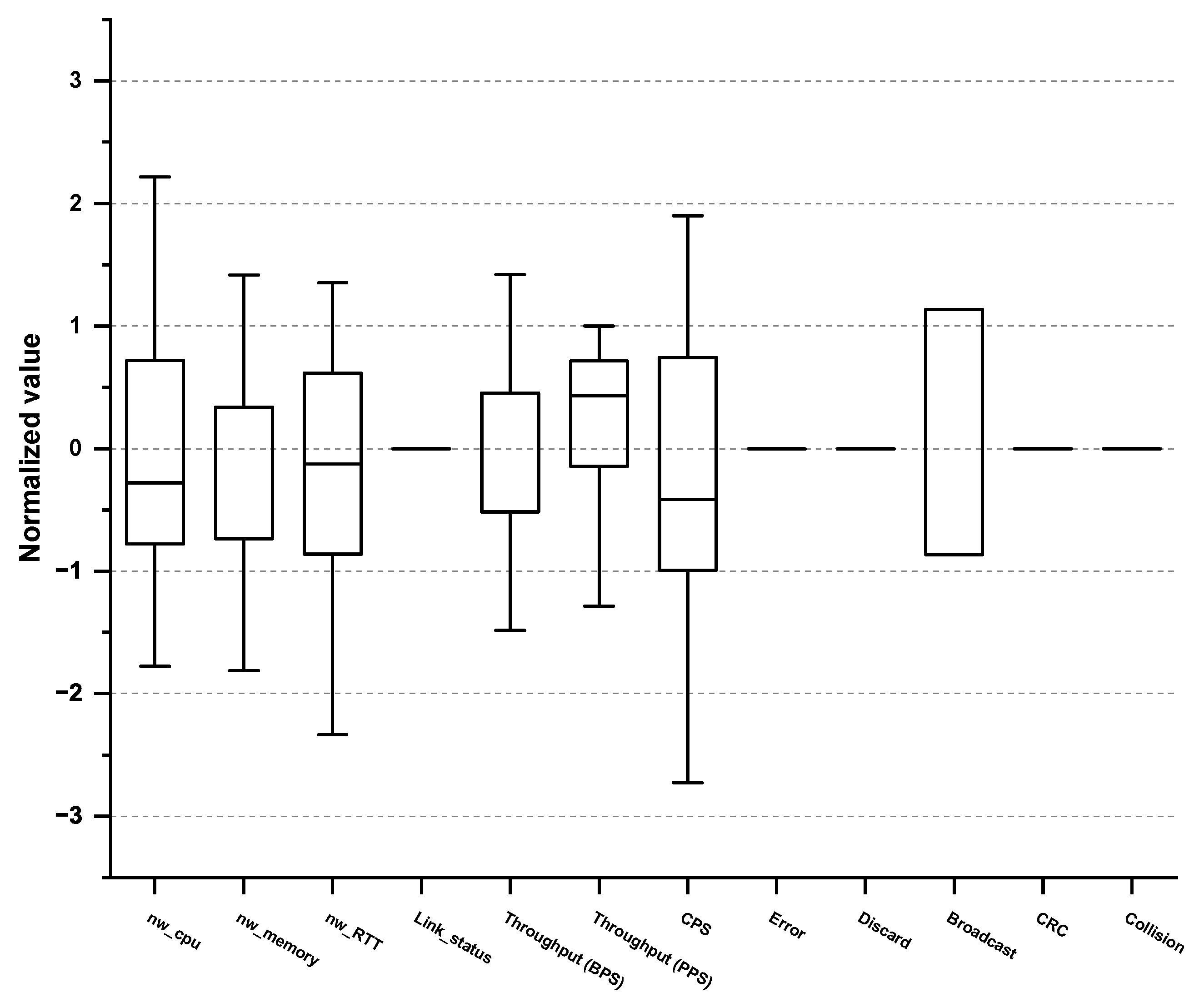
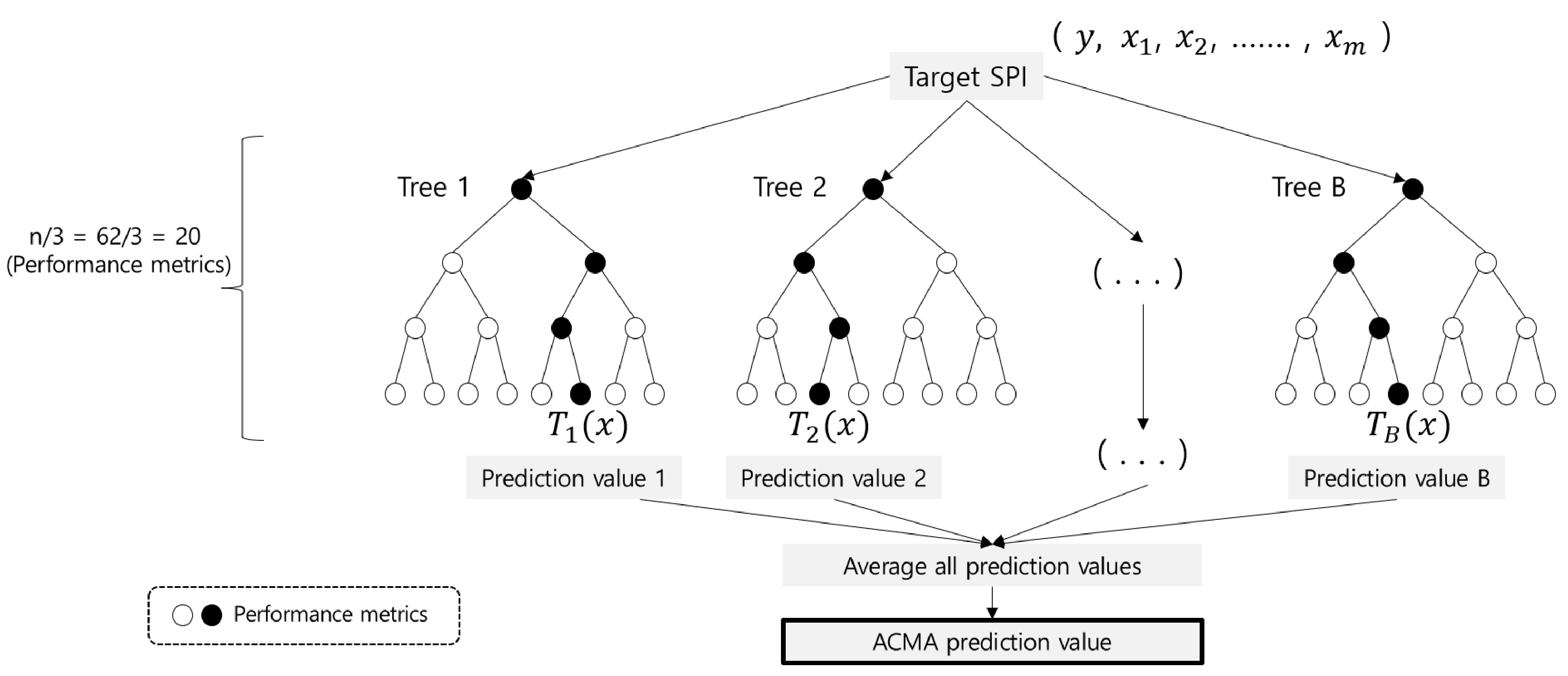
- We identified 62 vital PMs that contributed the most to the target SPI in a multitier enterprise infrastructure environment and provided their corresponding threshold values.
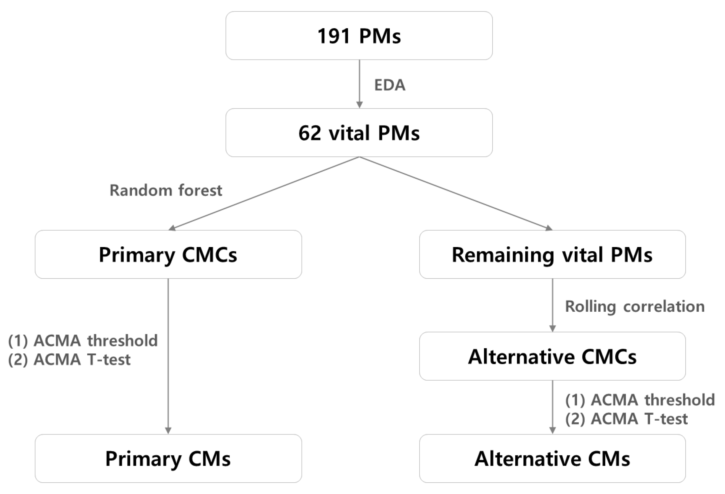
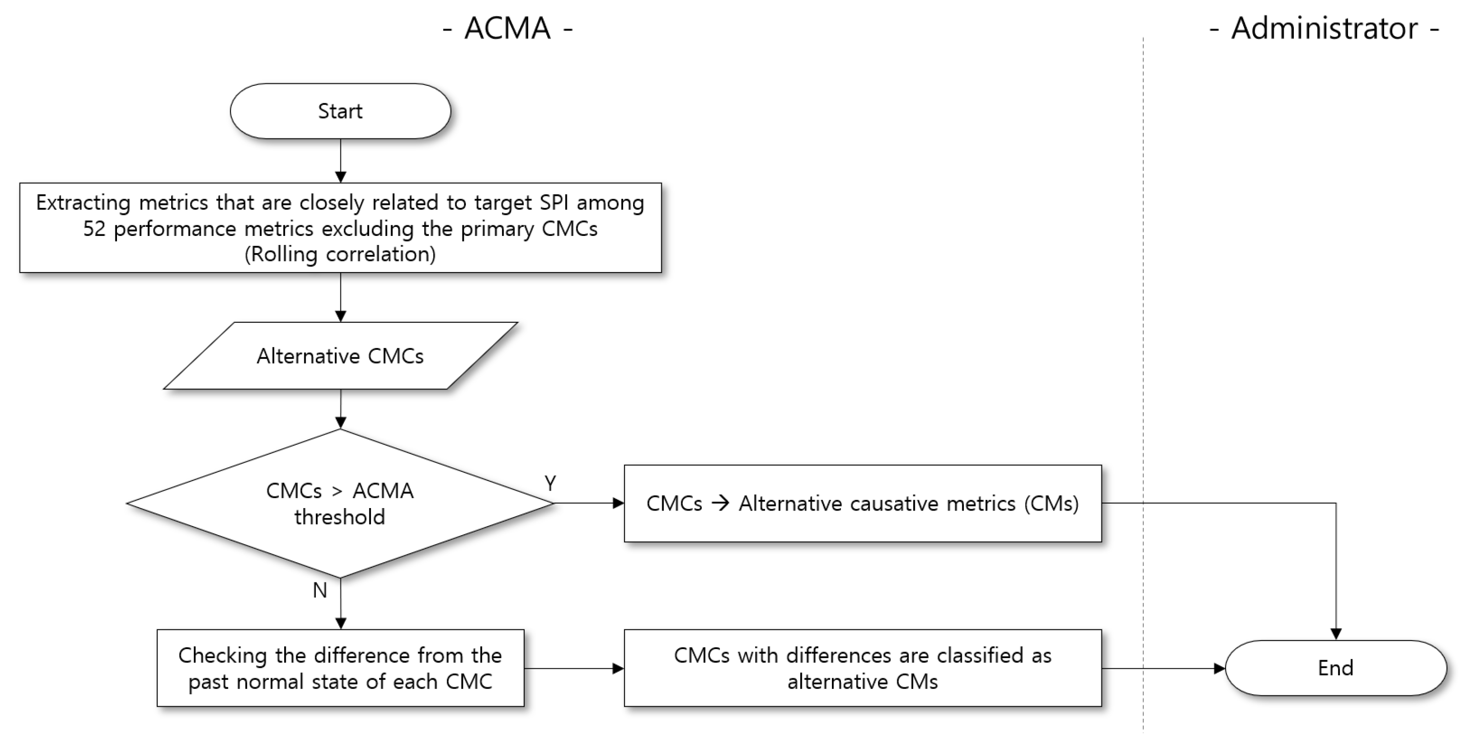
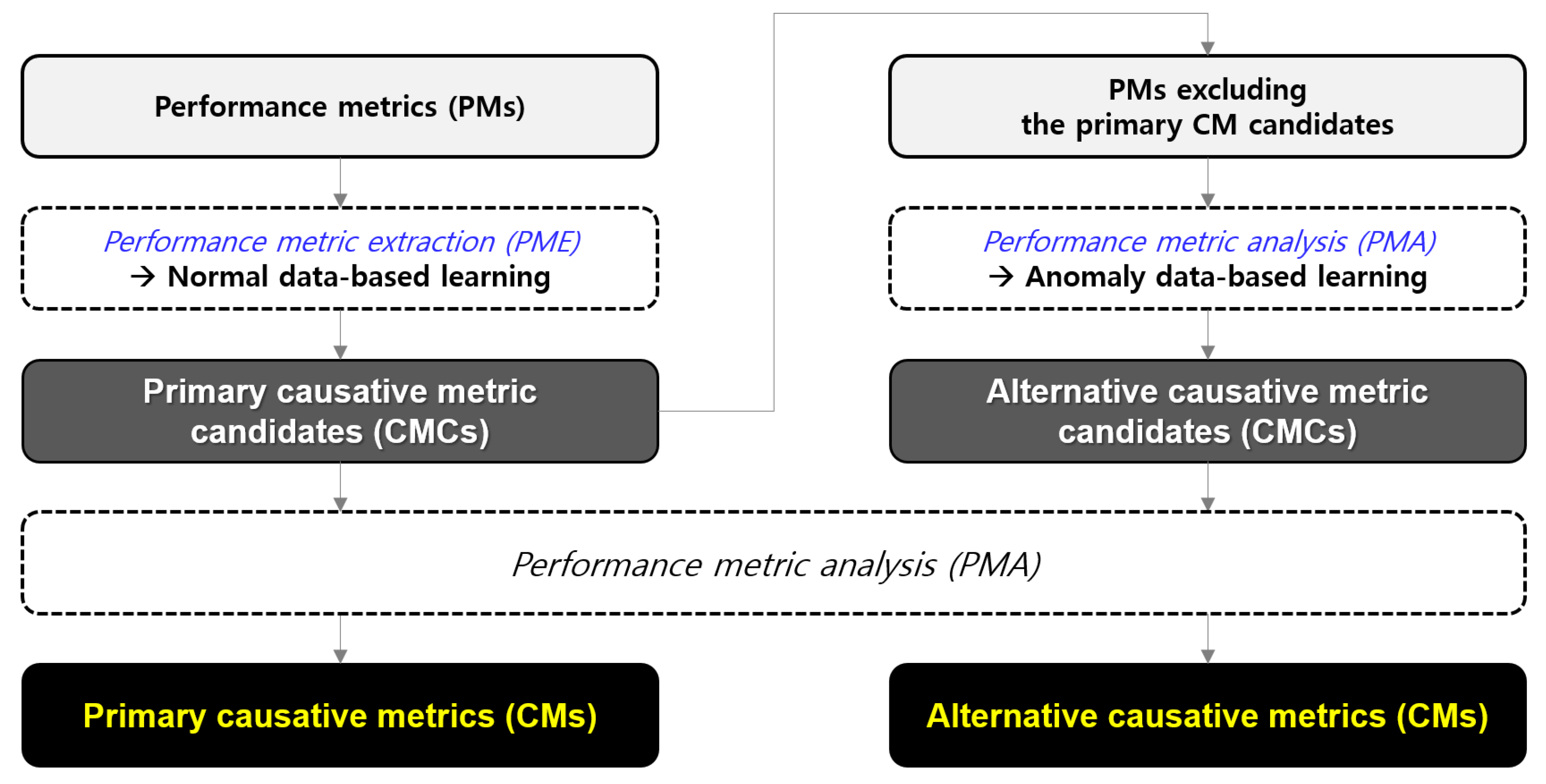
- Here, we present methods to extract the primary and alternative CM candidates from the vital PMs. Since navigating all the PMs is time-consuming, reducing the search space is necessary to derive the CMs related to the target SPI performance anomalies rapidly.
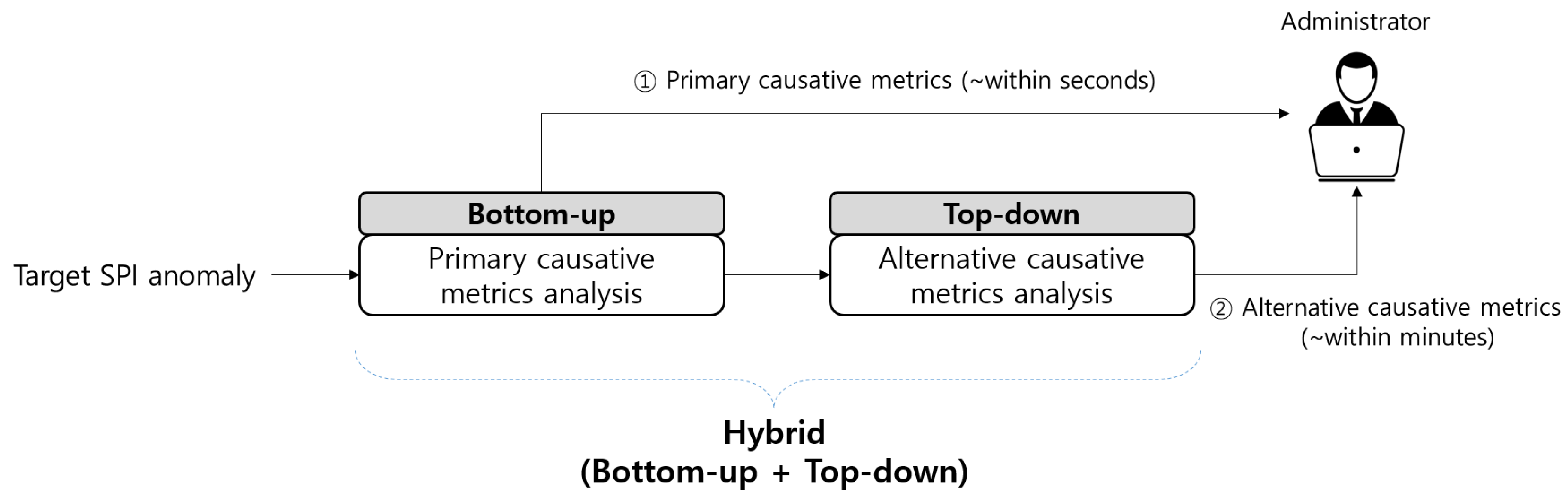
- We used several statistical methodologies to determine whether a performance anomaly is related to the primary or alternative CM candidates, thereby bridging the gap between anomaly detection and root cause analysis. Notably, most of the existing methods adopt a top-down approach to detect outliers in the target SPI first and subsequently launch a root cause analysis, which involves multiple iterations of validation against a large amount of PMs.
- We evaluated the effectiveness of our approach by using enterprise services. The experimental results demonstrated that the ACMA can provide the CM candidates immediately, thereby aiding the service administrator in identifying the potential causes. Based on the results obtained by implementing the ACMA to enterprise services, we conclude that the ACMA can provide deeper insights into the performance anomalies and enhance service reliability.
2. Preliminaries
2.1. PMs and Target SPI
2.2. CMCs and CMs of Performance Anomaly
2.3. Problem Definition
3. Proposed Method: ACMA
3.1. Motivating Example
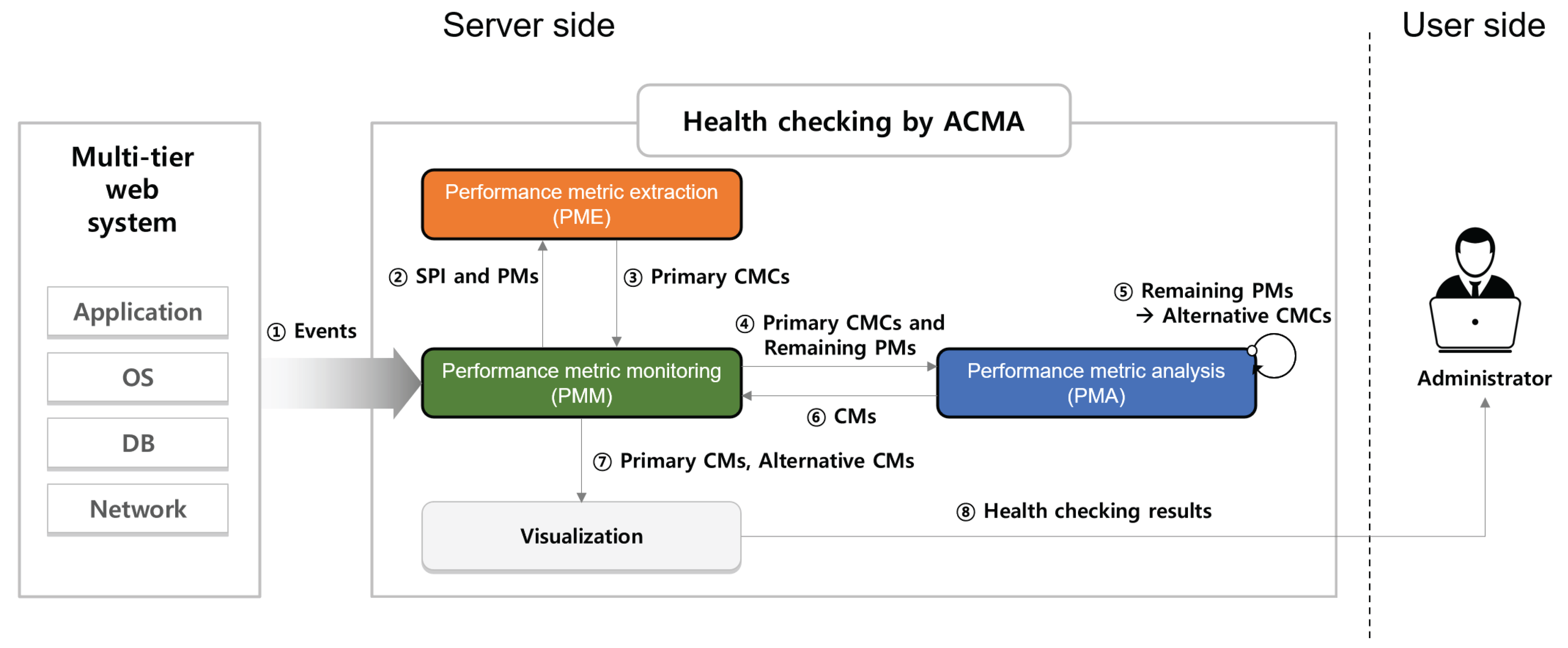
3.2. Health Check of the Target SPI
3.3. PMs of the ACMA
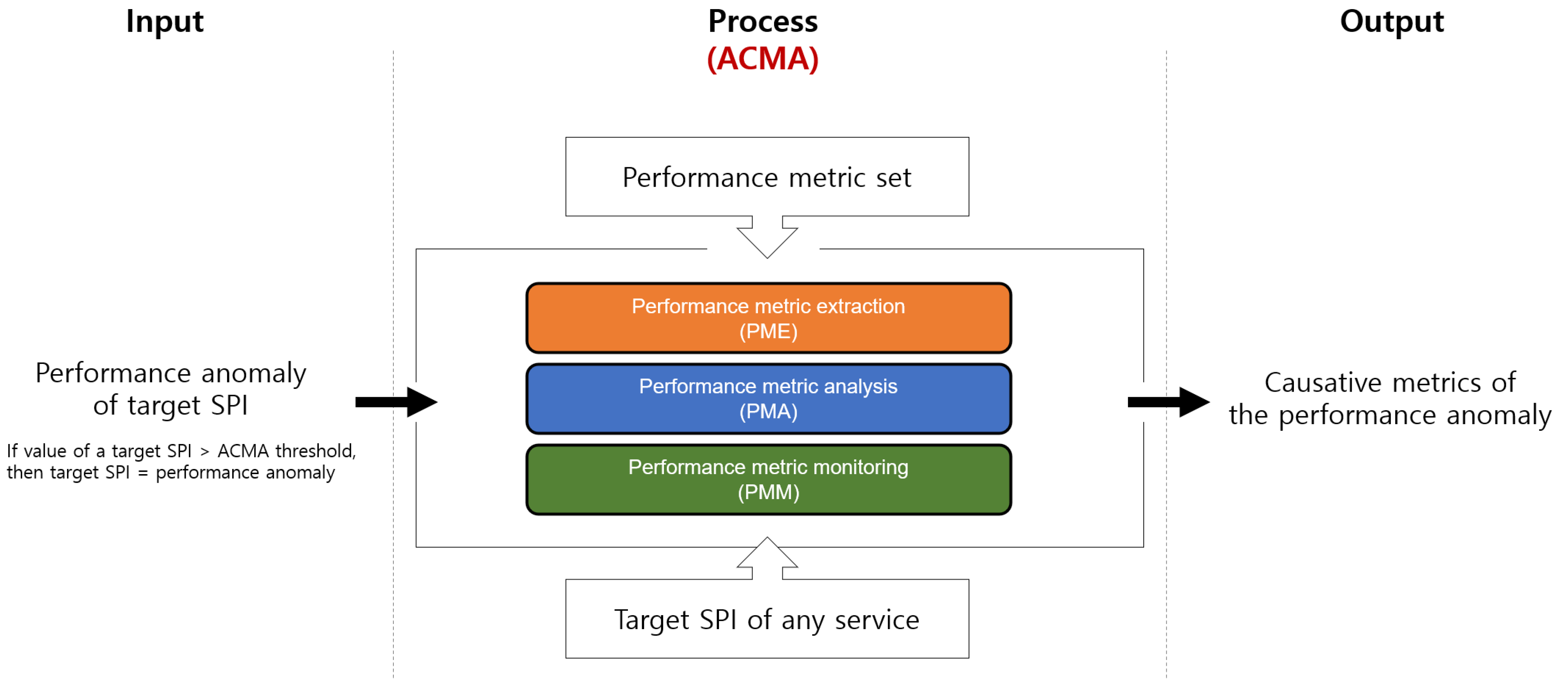
3.4. Overview of the ACMA
4. Description of Acma Components
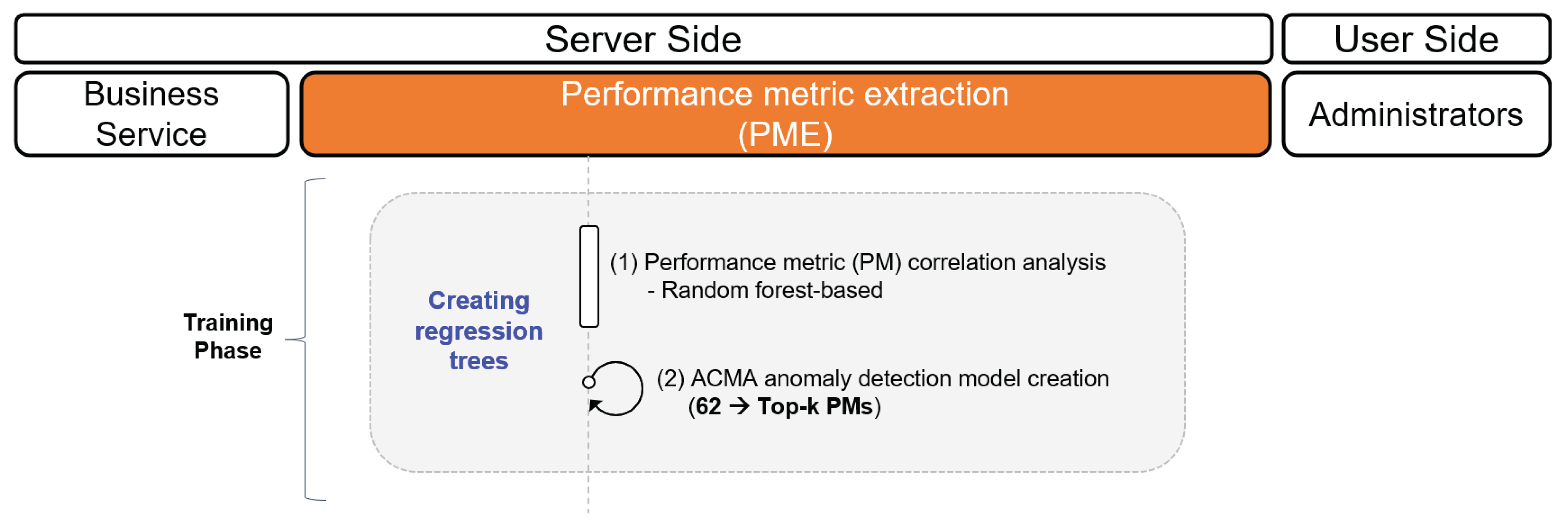
4.1. Performance Metric Extraction (PME)
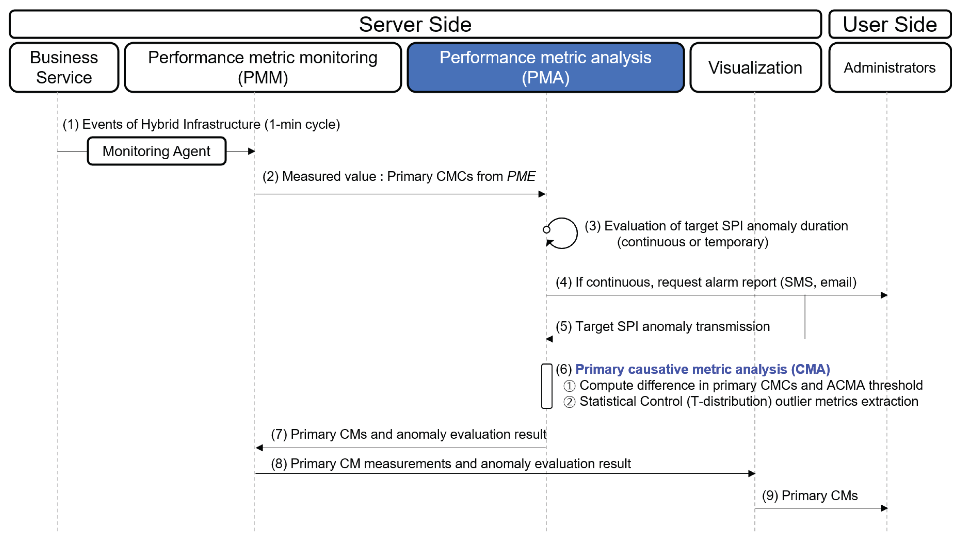
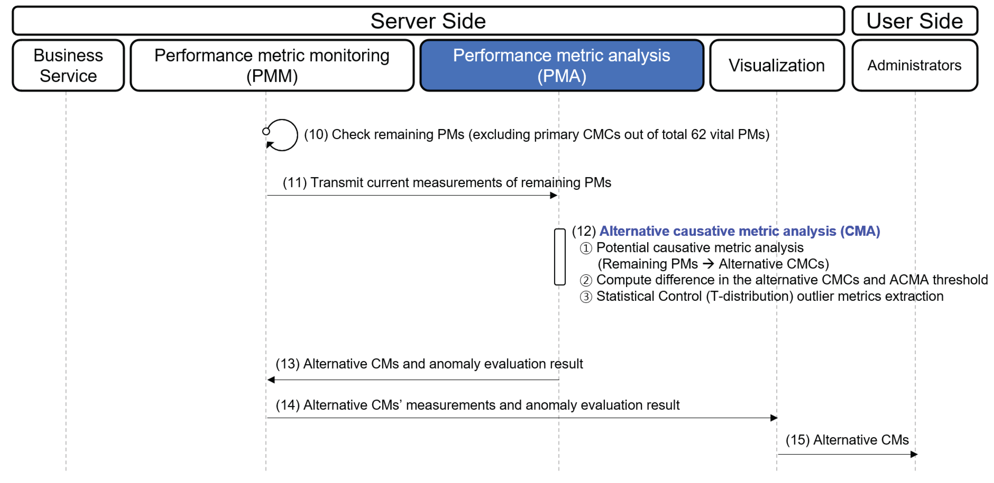
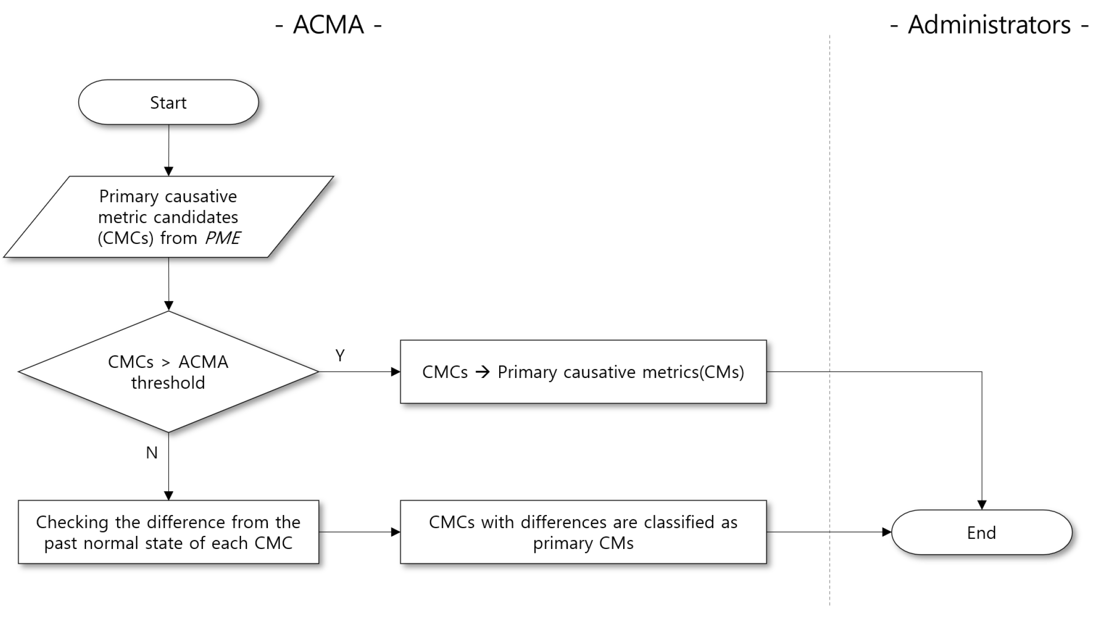
4.2. Performance Metric Analysis (PMA)
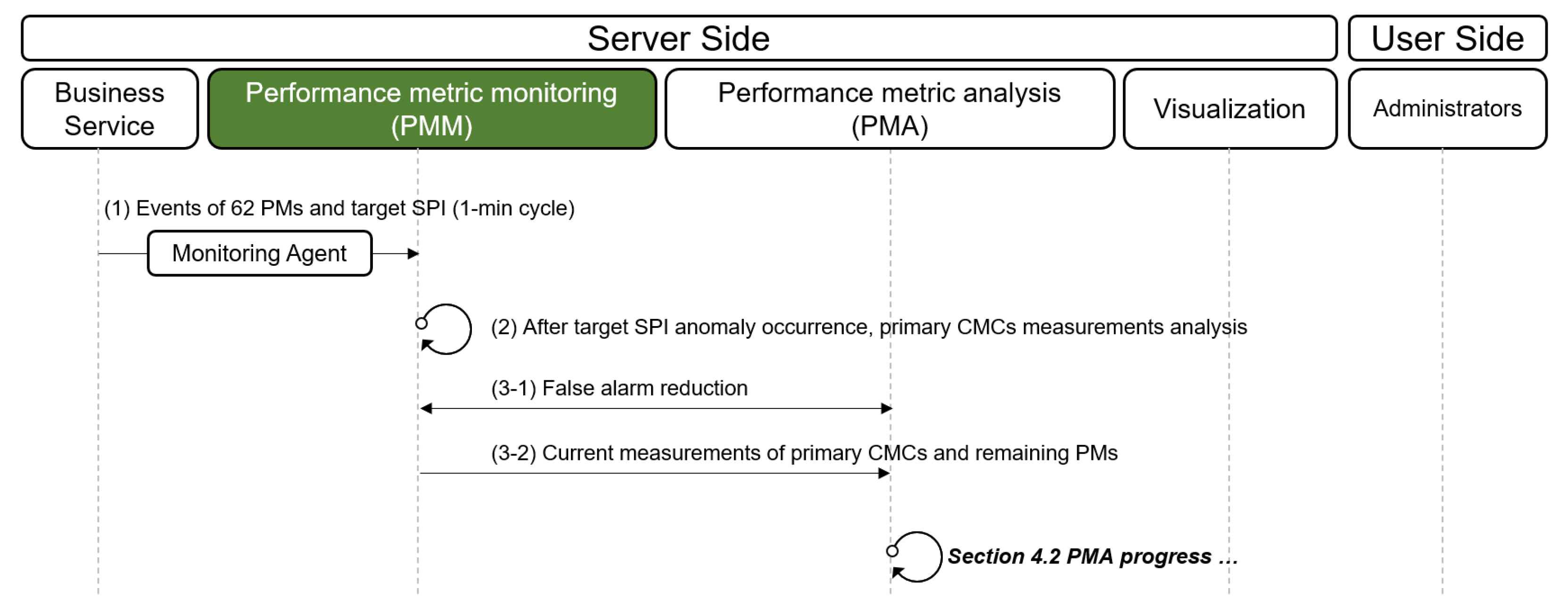
4.3. Performance Metric Monitoring (PMM)
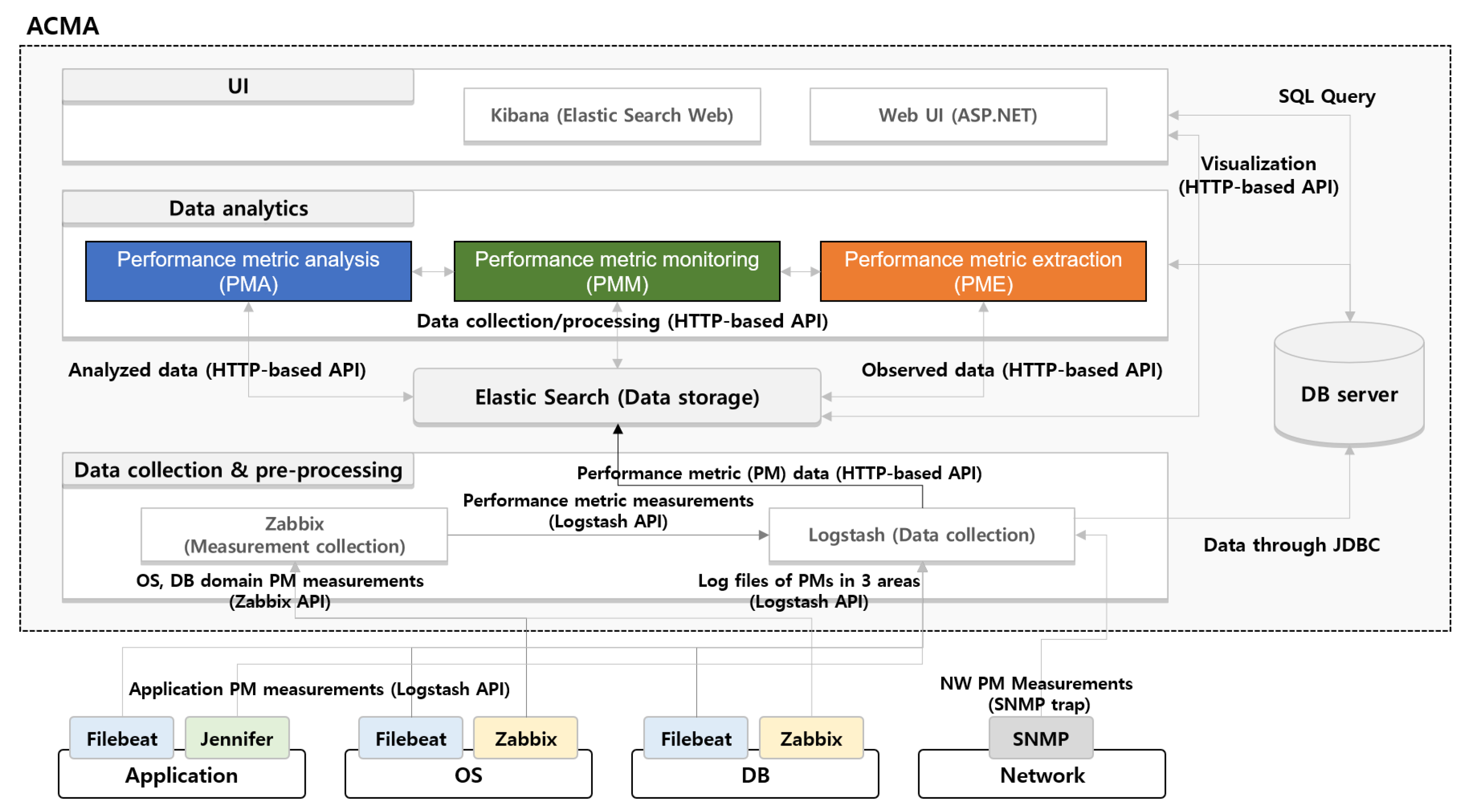
4.4. Implementation of the ACMA Framework
5. Evaluation
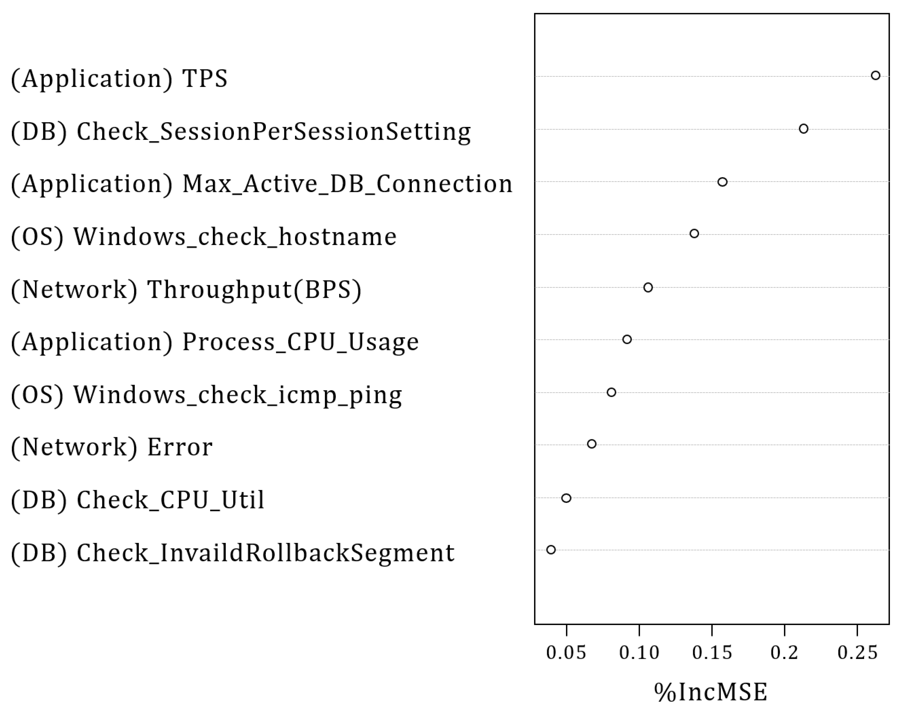
5.1. CMCs in Experimental Settings
5.2. Case Studies
5.3. Evaluation of the Accuracy of Anomaly Detection
5.3.1. Experimental Settings
5.3.2. Experimental Results
5.4. Evaluation of the Quality of Root Cause Analysis
5.4.1. Experimental Settings
5.4.2. Experimental Results
6. Related Work
7. Conclusions
Author Contributions
Funding
Institutional Review Board Statement
Informed Consent Statement
Data Availability Statement
Conflicts of Interest
References
- Ibidunmoye, O.; Hernández-Rodriguez, F.; Elmroth, E. Performance anomaly detection and bottleneck identification. ACM Comput. Surv. 2015, 48, 1–35. [Google Scholar] [CrossRef]
- Ren, H.; Xu, B.; Wang, Y.; Yi, C.; Huang, C.; Kou, X.; Xing, T.; Yang, M.; Tong, J.; Zhang, Q. Time-series anomaly detection service at microsoft. In Proceedings of the 25th ACM SIGKDD International Conference on Knowledge Discovery & Data Mining, Anchorage, AK, USA, 4–8 August 2019; pp. 3009–3017. [Google Scholar]
- Laptev, N.; Amizadeh, S.; Flint, I. Generic and scalable framework for automated time-series anomaly detection. In Proceedings of the 21th ACM SIGKDD International Conference on Knowledge Discovery and Data Mining, Sydney, NSW, Australia, 10–13 August 2015; pp. 1939–1947. [Google Scholar]
- Peiris, M.; Hill, J.H.; Thelin, J.; Bykov, S.; Kliot, G.; Konig, C. Pad: Performance anomaly detection in multi-server distributed systems. In Proceedings of the 2014 IEEE 7th International Conference on Cloud Computing, Anchorage, AK, USA, 27 June–2 July 2014; pp. 769–776. [Google Scholar]
- Jennifersoft Inc. 2021. Available online: https://jennifersoft.com/en/ (accessed on 9 June 2022).
- Samsung SDS. The Multi-Tier Web System of Samsung Virtual Private Network (SVPN). 2021. Available online: https://www.samsungvpn.com (accessed on 16 June 2022).
- Samsung SDS. The Multi-Tier Web System of Samsung uReady. 2021. Available online: http://www.samsunguready.com (accessed on 16 June 2021).
- Wilcox, R.R. Introduction to Robust Estimation and Hypothesis Testing, 4th ed.; Academic Press: Cambridge, MA, USA, 2017. [Google Scholar]
- Global Wep Application Market Share. 2019. Available online: https://hostadvice.com/marketshare/server/ (accessed on 12 December 2022).
- Gartner. Market Share Analysis: Server Operating Systems, Worldwide. 2017. Available online: https://www.gartner.com/en/documents/3883365 (accessed on 10 December 2022).
- Cisco. SNMP Configuration Guide. 2021. Available online: https://www.cisco.com/c/en/us/td/docs/ios-xml/ios/snmp/configuration/xe-16/snmp-xe-16-book/nm-snmp-cfg-snmp-support.html (accessed on 10 December 2022).
- F5. Configuring SNMP. 2022. Available online: https://support.f5.com/csp/article/K52219241 (accessed on 12 December 2022).
- Juniper. Configuring Basic SNMP. 2021. Available online: https://www.juniper.net/documentation/us/en/software/junos/network-mgmt/topics/topic-map/configuring-basic-snmp.html (accessed on 10 December 2022).
- Mauro, D.; Schmidt, K. Essential SNMP: Help for System and Network Administrators; O’Reilly Media, Inc.: Sebastopol, CA, USA, 2005. [Google Scholar]
- Stallings, W. SNMP, SNMPv2, SNMPv3, and RMON 1 and 2; Addison-Wesley Longman Publishing Co., Inc.: Boston, MA, USA, 1998. [Google Scholar]
- Gartner. Market Share: Database Management Systems, Worldwide. 2019. Available online: https://www.gartner.com/en/documents/4001330 (accessed on 9 June 2022).
- Filebeat Overview. 2021. Available online: https://www.elastic.co/guide/en/beats/filebeat/current/filebeat-overview.html (accessed on 9 June 2022).
- Zabbix LLC. 2021. Available online: https://www.zabbix.com/ (accessed on 9 June 2022).
- Spark Apache. 2021. Available online: http://spark.apache.org/docs/latest/mllib-decision-tree.html (accessed on 12 December 2022).
- Kamiński, B.; Jakubczyk, M.; Szufel, P. A framework for sensitivity analysis of decision trees. Cent. Eur. J. Oper. Res. 2018, 26, 135–159. [Google Scholar] [CrossRef] [PubMed]
- Deng, H.; Runger, G.; Tuv, E. Bias of importance measures for multi-valued attributes and solutions. In Proceedings of the International Conference on Artificial Neural Networks, Espoo, Finland, 14–17 June 2011; pp. 293–300. [Google Scholar]
- Ye, H.; Qu, X.; Liu, S.; Li, G. Hybrid sampling method for autoregressive classification trees under density-weighted curvature distance. Enterp. Inf. Syst. 2021, 15, 749–768. [Google Scholar] [CrossRef]
- Liaw, A.; Wiener, M. Classification and regression by randomForest. R News 2002, 2, 18–22. [Google Scholar]
- Zhu, R.; Zeng, D.; Kosorok, M.R. Reinforcement learning trees. J. Am. Stat. Assoc. 2015, 110, 1770–1784. [Google Scholar] [CrossRef] [PubMed]
- Painsky, A.; Rosset, S. Cross-validated variable selection in tree-based methods improves predictive performance. IEEE Trans. Pattern Anal. Mach. Intell. 2016, 39, 2142–2153. [Google Scholar] [CrossRef] [PubMed]
- Vidal, T.; Schiffer, M. Born-again tree ensembles. In Proceedings of the International Conference on Machine Learning (PMLR’20), Online, 26–28 August 2020; pp. 9743–9753. [Google Scholar]
- Hastie, T.; Tibshirani, R.; Friedman, J. The Elements of Statistical Learning: Data Mining, Inference, and Prediction; Springer Science & Business Media: Berlin/Heidelberg, Germany, 2009. [Google Scholar]
- Derrick, B. How to compare the means of two samples that include paired observations and independent observations: A companion to Derrick, Russ, Toher and White (2017). Quant. Methods Psychol. 2017, 13, 120–126. [Google Scholar] [CrossRef]
- Raju, T.N. William Sealy Gosset and William A. Silverman: Two “students” of science. Pediatrics 2005, 116, 732–735. [Google Scholar] [CrossRef] [PubMed]
- Walpole, R.E.; Myers, R.H.; Myers, S.L.; Ye, K. Probability and Statistics for Engineers and Scientists; Macmillan: New York, NY, USA, 1993; Volume 5. [Google Scholar]
- Bevans, R. T-Distribution: What It Is and How to Use It. 2021. Available online: https://www.scribbr.com/statistics/t-distribution/ (accessed on 12 December 2022).
- Weisstein, E.W. Statistical Correlation. 2020. Available online: https://mathworld.wolfram.com/StatisticalCorrelation.html (accessed on 10 December 2022).
- SPSS Tutorials. Statistical Pearson Correlation. 2021. Available online: https://libguides.library.kent.edu/SPSS/PearsonCorr (accessed on 10 December 2022).
- Elasticsearch Guide. 2021. Available online: https://www.elastic.co/guide/en/elasticsearch/reference/current/rest-apis.html (accessed on 10 December 2022).
- Filebeat API. 2021. Available online: https://www.elastic.co/guide/en/beats/filebeat/current/http-endpoint.html (accessed on 10 December 2022).
- Jennifer API. 2021. Available online: https://github.com/jennifersoft/jennifer-server-view-api-oam (accessed on 10 December 2022).
- Zabbix API. 2021. Available online: https://www.zabbix.com/documentation/current/manual/api (accessed on 10 December 2022).
- Logstash. 2021. Available online: https://www.elastic.co/guide/en/logstash/current/plugins-inputs-snmp.html (accessed on 10 December 2022).
- Kibana Guide. 2021. Available online: https://www.elastic.co/guide/en/kibana/master/api.html (accessed on 10 December 2022).
- Liu, D.; Zhao, Y.; Xu, H.; Sun, Y.; Pei, D.; Luo, J.; Jing, X.; Feng, M. Opprentice: Towards practical and automatic anomaly detection through machine learning. In Proceedings of the 2015 Internet Measurement Conference, Tokyo, Japan, 28–30 October 2015; pp. 211–224. [Google Scholar]
- Xu, H.; Chen, W.; Zhao, N.; Li, Z.; Bu, J.; Li, Z.; Liu, Y.; Zhao, Y.; Pei, D.; Feng, Y.; et al. Unsupervised anomaly detection via variational auto-encoder for seasonal kpis in web applications. In Proceedings of the 2018 World Wide Web Conference, Lyon, France, 23–27 April 2018; pp. 187–196. [Google Scholar]
- Shipmon, D.T.; Gurevitch, J.M.; Piselli, P.M.; Edwards, S.T. Time series anomaly detection; detection of anomalous drops with limited features and sparse examples in noisy highly periodic data. arXiv 2017, arXiv:1708.03665. [Google Scholar]
- Vallis, O.; Hochenbaum, J.; Kejariwal, A. A Novel for LongTerm Anomaly Detection in the Cloud. In Proceedings of the 6th USENIX Workshop on Hot Topics in Cloud Computing (HotCloud’14), Philadelphia, PA, USA, 17–18 June 2014. [Google Scholar]
- Kim, S.; Suh, I.; Chung, Y.D. Automatic monitoring of service reliability for web applications: A simulation-based approach. Softw. Test. Verif. Reliab. 2020, 30, e1747. [Google Scholar] [CrossRef]
- Kavulya, S.P.; Daniels, S.; Joshi, K.; Hiltunen, M.; Gandhi, R.; Narasimhan, P. Draco: Statistical diagnosis of chronic problems in large distributed systems. In Proceedings of the IEEE/IFIP International Conference on Dependable Systems and Networks (DSN 2012), Boston, MA, USA, 25–28 June 2012; pp. 1–12. [Google Scholar]
- Nagaraj, K.; Killian, C.; Neville, J. Structured comparative analysis of systems logs to diagnose performance problems. In Proceedings of the 9th USENIX Symposium on Networked Systems Design and Implementation (NSDI’12), San Jose, CA, USA, 25–27 April 2012; pp. 353–366. [Google Scholar]
- Roy, S.; König, A.C.; Dvorkin, I.; Kumar, M. Perfaugur: Robust diagnostics for performance anomalies in cloud services. In Proceedings of the 2015 IEEE 31st International Conference on Data Engineering, Seoul, Republic of Korea, 13–17 April 2015; pp. 1167–1178. [Google Scholar]
- Nguyen, H.; Tan, Y.; Gu, X. Pal: Propagation-aware anomaly localization for cloud hosted distributed applications. In Proceedings of the Managing Large-Scale Systems via the Analysis of System Logs and the Application of Machine Learning Techniques, Cascais, Portugal, 23–26 October 2011; pp. 1–8. [Google Scholar]
- Jayathilaka, H.; Krintz, C.; Wolski, R. Performance monitoring and root cause analysis for cloud-hosted web applications. In Proceedings of the 26th International Conference on World Wide Web, Perth, WA, Australia, 3–7 April 2017; pp. 469–478. [Google Scholar]


| ENS | Number of PMs | Total PMs | Search Space for Finding CMs | Average Time for Finding CMs | |||
|---|---|---|---|---|---|---|---|
| Applications | DB | OSs | Network | ||||
| ENS1 | 57 | 31 | 58 | 45 | 191 | 6.5 days | |
| ENS2 | 41 | 29 | 57 | 59 | 186 | 5 days | |
| No. | Performance Metric | Descriptions | Threshold | Monitoring Cycle |
|---|---|---|---|---|
| 1 | Process_CPU_Usage (%) | CPU utilization of the process being monitored | value | 1 s |
| 2 | Process_Mem_Usage (MB) | Memory utilization of the process being monitored (e.g., JVM process memory usage for Java) | value | 1 s |
| 3 | Heap Memory Usage (%) | Measuring the allocating size of the Java Virtual Machine(JVM) heap memory area | value | 1 s |
| 4 | Current_Thread | The number of created threads | value | 1 s |
| 5 | GC_Time (ms) | Garbage collection (GC) time | value | 1 s |
| 6 | GC Activity (%) | Percentage of garbage collection usage time | value | 1 s |
| 7 | Active users | The number of users actually executing the transaction | value | 1 min |
| 8 | TPS | Transactions per second | value | 1 s |
| 9 | CPU_Time_per_Transaction | CPU time used during a transaction | value | 1 min |
| 10 | Active_SQL | Number of the SQL statement | value | 1 s |
| 11 | SQL_per_Transaction | Total number of SQL calls divided by the number of transactions | value | 1 min |
| 12 | External_Call_Time (ms) | Average execution time of one external call | value | 1 min |
| 13 | Fetch_Number | Sum of numbers measured by fetch | value < 10,000 | 1 min |
| 14 | Fetch_Time (ms) | Average execution time per fetch | value < 10,000 | 1 min |
| 15 | Max_Active_DB_Connection | Maximum number of active DB connections | value | 1 s |
| No. | Performance Metric | Descriptions | Threshold | Monitoring Cycle |
|---|---|---|---|---|
| 1 | WindowsCheck_hostname | Hostname consistency check | 1 or more non-response | 1 min |
| 2 | WindowsCheck_icmp_ping | Internet Control Message Protocol (ICMP) ping status to a Windows server | 1 or more non-response | 1 min |
| 3 | WindowsCheck_wcpu_processorTime | Percentage of time the processor runs non-idle threads | 90% | 1 min |
| 4 | WindowsCheck_weventlog_usage | The ratio of the used capacity to the total capacity of the event log | 96% | 5 min |
| 5 | WindowsCheck_wld_free_space_pct | Percentage of free space available on the logical disk drive | 15% or less | 5 min |
| 6 | WindowsCheck_wmem_usage | The ratio of the used capacity to the total memory capacity (Windows) | 90% | 1 min |
| 7 | Linux_check_sys | Percentage of CPU time spent in user mode(usr) + Percentage of CPU time spent in system mode(sys) | 90% | 1 min |
| 8 | Linux_check_cpu_usage | CPU time spent on system tasks | 80% | 1 min |
| 9 | Linux_check_user_memory_usage | The ratio of the used capacity to the total memory capacity (Linux) | 90% | 1 min |
| 10 | Linux_check_file_pct | Percentage of the filesystem in use | 90% | 1 min |
| 11 | Linux_check_inode_pct | Percentage of inodes allocated | 90% | 1 min |
| 12 | Linux_check_usage | Percentage of capacity in use to total swap capacity | 70% | 1 min |
| 13 | Linux_check_icmp_ping | Internet Control Message Protocol (ICMP) ping status to a Linux server | 1 or more non-response | 1 min |
| No. | Performance Metric | Descriptions | Threshold | Monitoring Cycle |
|---|---|---|---|---|
| 1 | nw_cpu | CPU utilization | 80% | 1 min |
| 2 | nw_memory | Memory utilization | 80% | 1 min |
| 3 | nw_RTT | Ping check whether the device is accessible | 1 ms per 100 km | 1 s |
| 4 | Link_status | Check for port link status | Up/Down | 1 s |
| 5 | Throughput (BPS) | Bandwidth—Min/Avg/Max (Bits per second, BPS) | 80% | 1 min |
| 6 | Throughput (PPS) | Packet throughput—Min/Avg/Max (Packets per second, PPS) | 80% | 1 min |
| 7 | CPS | Session throughput—Min/Avg/Max (Character per second, CPS) | 90% | 1 min |
| 8 | Error | Packet(In/Out) error rate | 1% | 1 min |
| 9 | Discard | Checking for discarded packets due to insufficient buffer | 1% | 1 min |
| 10 | Broadcast | Received broadcast packet monitoring | 0.50% | 1 min |
| 11 | CRC | The number of packets with abnormal CRC value through packet checksum (Cyclic redundancy check, CRC) | 1% | 1 min |
| 12 | Collision | Number of packets retransmitted due to Ethernet collision | 1% | 1 min |
| No. | Performance Metric | Descriptions | Threshold | Monitoring Cycle |
|---|---|---|---|---|
| 1 | RedologFileStatus | Redo log file status (0: Normal, 100: Warning) | value = 100 | 1440 min |
| 2 | CountOfDFPerDBfiles | The number of current datafiles/DB_FILES * 100 | 80 ≤ value < 90 | 1440 min |
| 3 | TableSpaceFreeSpace | Table space available space—DATAFILE ≤ Threshold | value ≤ 1024 M | 60 min |
| 4 | lib_pin_cnt | The number of pin events | 1 ≤ value < 5 | 1 min |
| 5 | local_dbconn_status | Connection check in the DB server (1: Normal, 0: Failure) | - | 1 min |
| 6 | waitingLock | Lock request time (max) | 5 ≤ value < 20 | 1 min |
| 7 | SessionlnLongLock | Lock holding time (max) | 5 ≤ value < 20 | 1 min |
| 8 | TableSpaceFreeSpacePct | The free percentage of tablespace | 5 ≤ value < 10 | 60 min |
| 9 | fra_usage | Flashback recovery area (FRA) usage rate | 80 ≤ value < 90 | 1 min |
| 10 | check_cpu_idle | CPU Idle time | 5 s or less | 1 min |
| 11 | check_cpu_runqueue | Number of processes in run queue | More than 10 | 1 min |
| 12 | check_cpu_util | Usage active on CPU | 90% | 1 min |
| 13 | check_fs_used_pct | Percentage of the filesystem in use | 85% | 5 min |
| 14 | check_inode_used_pct | Percentage of inodes in use | 90% | 5 min |
| 15 | check_mem_usage | The ratio of used capacity to total memory capacity | 90% | 1 min |
| 16 | check_CountOfDfPerDbfiles | (The number of current datafiles/DB_FILES) * 100 | 90% | 5 min |
| 17 | check_LockPerLockSetting | (Current DML_LOCKS / DML_LOCKS) * 100 | 90% | 5 min |
| 18 | check_ProcessPerProcessSetting | (Current Processes / Processes) * 100 | 90% | 5 min |
| 19 | check_SessionPerSessionSetting | (Current Sessions / Sessions) * 100 | 90% | 5 min |
| 20 | check_InvalidRollbackSegment | The status of the rollback segment | 80% | 5 min |
| 21 | check_proc_count | The average number of currently running processes | When 0 | 1 min |
| 22 | check_proc_cpuutil | CPU rate of the process at present | 90% | 1 min |
| ACMA Servers | Descriptions | |
|---|---|---|
| ACMA web server | OS | Windows server 2012 R2 standard edition |
| CPU | 4Core | |
| Memory | 16 GB | |
| Disk | 200 GB | |
| Model | Lenovo X3650 M5 | |
| ACMA analytics server | OS | CentOS 7.4.1708 |
| CPU | 8Core | |
| Memory | 16 GB | |
| Disk | 400 GB | |
| Model | Lenovo X3650 M5 | |
| ACMA search server | OS | CentOS 7.4.1708 |
| CPU | 8Core | |
| Memory | 16 GB | |
| Disk | 500 GB | |
| Model | Lenovo X3650 M5 | |
| ACMA collection server | OS | CentOS 7.4.1708 |
| CPU | 4Core | |
| Memory | 16 GB | |
| Disk | 500 GB | |
| Model | Lenovo X3650 M5 | |
| ACMA DB server | OS | Oracle Linux 7.2 |
| CPU | 16Core | |
| Memory | 64 GB | |
| Disk | 500 GB | |
| Model | DELL PowerEdge R930 | |
| Oracle Ver. | ORACLE 11g (11.2.0.4) | |
| Conditions | Descriptions | |
|---|---|---|
| Study subject | Samsung Virtual Private Network (SVPN) | |
| Key function | SVPN Authentication (www.samsungvpn.com) | |
| Target SPI | Response time | |
| Threshold of target SPI | 4 s | |
| Primary causative metric candidates | Application domain | Transaction Per Second (TPS) Max_Active_DB_Connection Process_CPU_Usage |
| OS domain | Windows_check_hostname Windows_check_icmp_ping | |
| Network domain | Throughput(BPS) error | |
| DB domain | Check_SessionPerSessionSetting Check_CPU_Util Check_InvaildRollbackSegment | |
| No. | Occurrence Date | Descriptions | Root Cause Location | Provided CMs (Rank) |
|---|---|---|---|---|
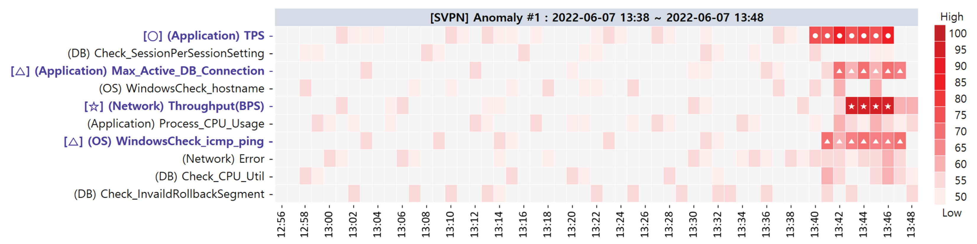
| 1 | 7 June 2022 13:38∼13:48 |
| Primary CMs | (Network) Throughput(BPS) (1st) (Application) TPS (2nd) (Application) Max_Active_DB_Connection (3rd) (OS) WindowsCheck_icmp_ping (3rd) |
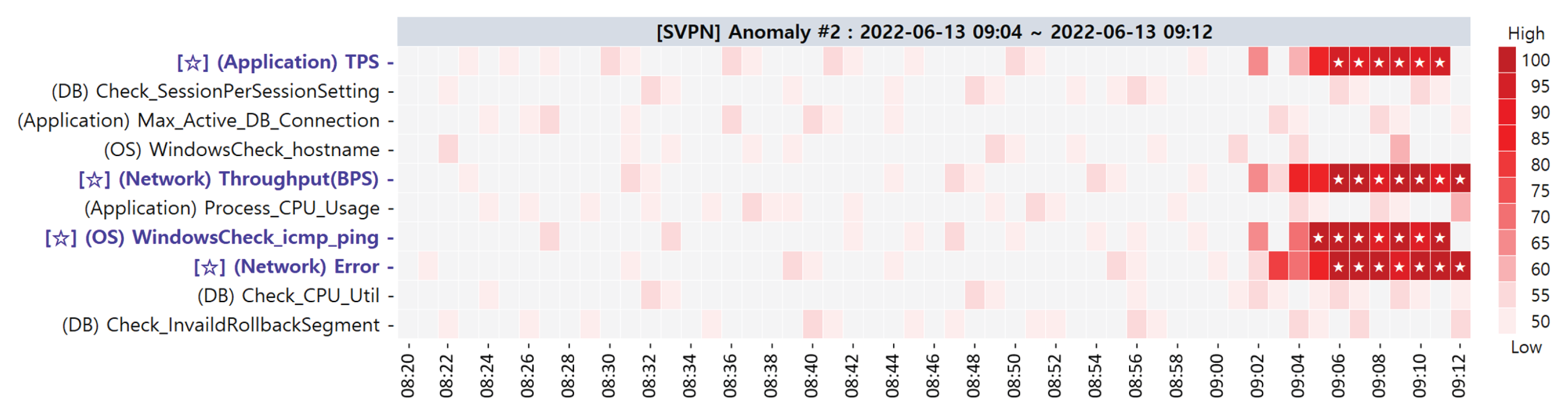
| 2 | 13 June 2022 09:04∼09:12 |
| Primary CMs | (Application) TPS (1st) (Network) Throughput(BPS) (1st) (OS) WindowsCheck_icmp_ping (1st) (Network) Error (1st) |
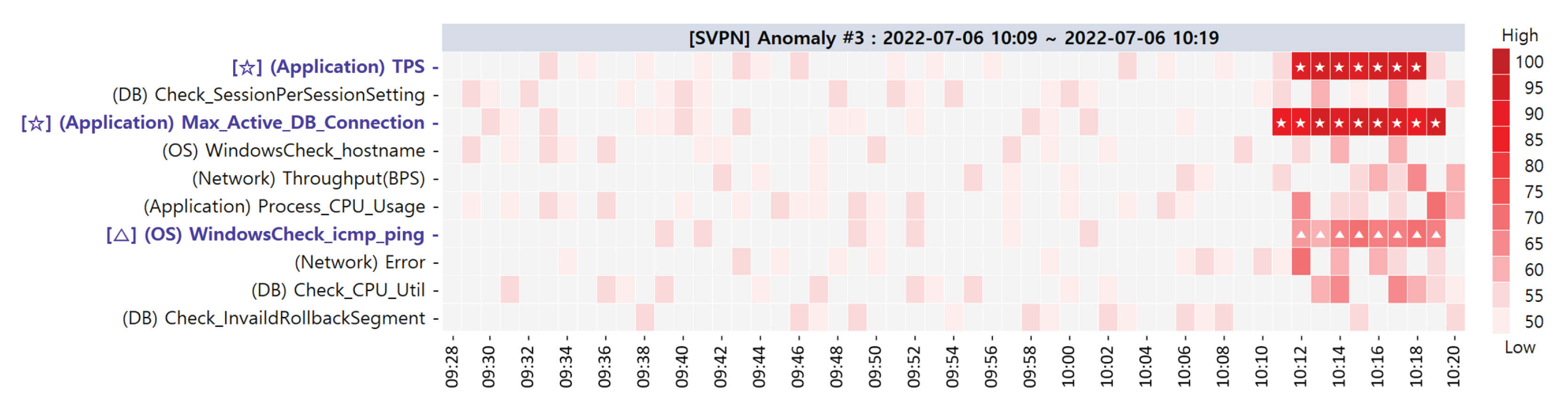
| 3 | 6 July 2022 10:09∼10:19 |
| Primary CMs | (Network) Throughput(BPS) (1st) (Application) Max_Active_DB_Connection (1st) (OS) WindowsCheck_icmp_ping (2nd) |
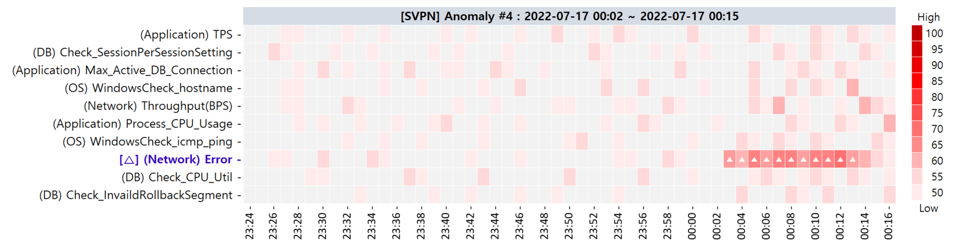
| 4 | 17 July 2022 00:02∼00:15 |
| Alternative CMs | (Network) CPS (1st) (Network) Discard (1st) (Network) Throughput(PPS) (1st) (Application) Process_Mem_Usage(MB) (2nd) (OS) WindowsCheck_wcpu_processorTime (2nd) (Application) Current_Thread (2nd) (Network) Collision (2nd) (Application) GC_Time(ms) (2nd) (Network) Error (3rd) |
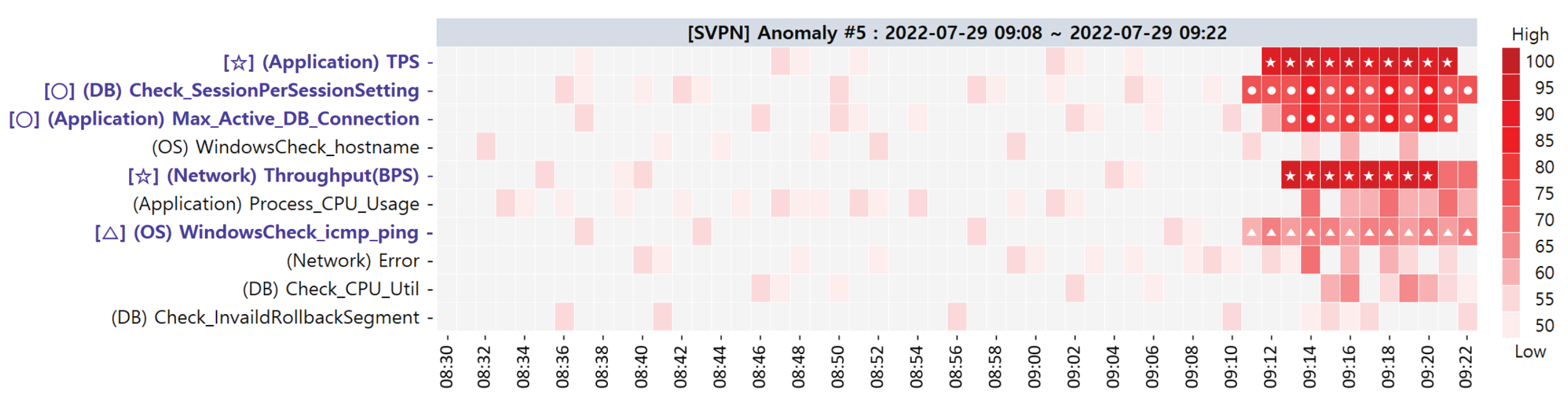
| 5 | 29 July 2022 09:08∼09:22 |
| Primary CMs | (Application) TPS (1st) (Network) Throughput(BPS) (1st) (DB) check_SessionPerSessionSetting (2nd) (Application) Max_Active_DB_Connection (2nd) (OS) WindowsCheck_icmp_ping (3rd) |
| 6 | 14 July 2022 13:02∼13:16 |
| None | None |
| No. | Performance Metric | Measured Value (Avg.) | Threshold | Monitoring Cycle |
|---|---|---|---|---|
| 1 | (OS) WindowsCheck_wmem_usage | 67% | 90% | 1 min |
| 2 | (Application) Active_SQL | 59 | 100 | 1 s |
| 3 | (OS) WindowsCheck_weventlog_usage | 61% | 96% | 5 min |
| 4 | (Network) Throughput(PPS) | 34% | 80% | 1 min |
| 5 | (Network) Collision | 0.29% | 1% | 1 min |
| 6 | (DB) WaitingLock | 11 | 20 | 1 s |
| 7 | (DB) SessionInLongLock | 7 | 20 | 1 s |
| 8 | (DB) Lib_pin_cnt | 2 | 5 | 1 s |
| 9 | (Application) Process_Mem_Usage | 1178 MB | 2048 MB | 1 s |
| 10 | (Application) Current_Thread | 47 | 100 | 1 s |
| No. | Performance Metric | Measured Value (Avg.) | Threshold | Monitoring Cycle |
|---|---|---|---|---|
| 1 | (Network) Throughput(PPS) | 82% | 80% | 1 min |
| 2 | (Network) CPS | 92% | 90% | 1 min |
| 3 | (Application) Current_Thread | 107 | 100 | 1 s |
| 4 | (Network) Discard | 0.9% | 1% | 1 min |
| 5 | (Network) Broadcast | 0.37% | 0.5% | 1 min |
| 6 | (Network) Collision | 0.86% | 1% | 1 min |
| 7 | (Application) Process_Mem_Usage (MB) | 1241 MB | 2048 MB | 1 s |
| 8 | (OS) WindowsCheck_wcpu_processorTime | 76% | 90% | 1 min |
| 9 | (Application) CPU_Time_per_Transaction | 2174 | 4000 | 1 min |
| 10 | (Application) Active_SQL | 59 | 100 | 1 s |
| No. | Performance Metric | Measured Value (Avg.) | Threshold | Monitoring Cycle |
|---|---|---|---|---|
| 1 | (OS) WindowsCheck_wmem_usage | 71% | 90% | 1 min |
| 2 | (Network) Throughput(PPS) | 52% | 80% | 1 min |
| 3 | (Application) Active_SQL | 49 | 100 | 1 s |
| 4 | (OS) WindowsCheck_weventlog_usage | 57% | 96% | 5 min |
| 5 | (Application) Process_Mem_Usage | 1096 MB | 2048 MB | 1 s |
| 6 | (Network) Collision | 0.21% | 1% | 1 min |
| 7 | (DB) WaitingLock | 9 | 20 | 1 s |
| 8 | (Application) Current_Thread | 53 | 100 | 1 s |
| 9 | (DB) SessionInLongLock | 7 | 20 | 1 s |
| 10 | (DB) Lib_pin_cnt | 1 | 5 | 1 s |
| No. | Performance Metric | Measured Value (Avg.) | Threshold | Monitoring Cycle |
|---|---|---|---|---|
| 1 | [✩] (Network) CPS | 93% | 90% | 1 min |
| 2 | [○] (Application) Process_Mem_Usage (MB) | 2072 | 2048 | 1 min |
| 3 | [○] (OS) WindowsCheck_wcpu_processorTime | 112 | 100 | 1 s |
| 4 | [✩] (Network) Discard | 1.23% | 1% | 1 min |
| 5 | [○](Application) Current_Thread | 107 | 100 | 1 min |
| 6 | [✩] (Network) Throughput(PPS) | 87% | 80% | 1 min |
| 7 | [○] (Network) Collision | 1.17% | 1% | 1 s |
| 8 | (Application) External_Call_Time(ms) | 4078 | 5000 | 1 min |
| 9 | [○] (Application) GC_Time (ms) | 1974 | 1000 | 1 min |
| 10 | (Application) GC Activity (%) | 2 | 3 | 1 s |
| No. | Performance Metric | Measured Value (Avg.) | Threshold | Monitoring Cycle |
|---|---|---|---|---|
| 1 | (OS) WindowsCheck_wmem_usage | 67% | 90% | 1 min |
| 2 | (Application) Active_SQL | 59 | 100 | 1 s |
| 3 | (OS) WindowsCheck_weventlog_usage | 61% | 96% | 5 min |
| 4 | (Network) Throughput(PPS) | 34% | 80% | 1 min |
| 5 | (Network) Collision | 0.29% | 1% | 1 min |
| 6 | (DB) WaitingLock | 11 | 20 | 1 s |
| 7 | (DB) SessionInLongLock | 7 | 20 | 1 s |
| 8 | (DB) Lib_pin_cnt | 2 | 5 | 1 s |
| 9 | (Application) Process_Mem_Usage | 1178 MB | 2048 MB | 1 s |
| 10 | (Application) Current_Thread | 47 | 100 | 1 s |
| ENS | PMs of a Multitier Web System | Approach for Finding CMs | Search Space for Finding CMs | Avg. Time for Finding CMs | |||
|---|---|---|---|---|---|---|---|
| App. PMs | DB PMs | OS PMs | NW PMs | ||||
| ENS | 57 | 31 | 58 | 45 | Top-down | 6.5 days | |
| ENS via ACMA | 15 | 22 | 13 | 12 | Primary CMCs → CMs: Bottom-up / Alternative CMCs → CMs: Top-down | Bottom-up: 10 from / Top-down: 52 from | If primary CMCs → CMs, then one minute / If alternative CMCs → CMs, then seven minutes |
| Anomaly Case | Anomaly #1 | Anomaly #2 | Anomaly #3 | Anomaly #4 | Anomaly #5 | |||||
|---|---|---|---|---|---|---|---|---|---|---|
| Method | ACMA | PAD | ACMA | PAD | ACMA | PAD | ACMA | PAD | ACMA | PAD |
| NDCG@5 | 0.88 | 0.15 | 0.97 | 0.15 | 0.97 | 0.38 | 0.83 | 0.17 | 1 | 0.14 |
| NDCG@10 | 0.9 | 0.34 | 0.94 | 0.14 | 0.98 | 0.47 | 0.85 | 0.31 | 0.98 | 0.38 |
| NDCG@15 | 0.9 | 0.43 | 0.98 | 0.3 | 0.99 | 0.5 | 0.86 | 0.45 | 0.99 | 0.38 |
| NDCG@20 | 0.91 | 0.48 | 0.98 | 0.43 | 0.99 | 0.49 | 0.87 | 0.5 | 1 | 0.46 |
| Technique | Methodology | Performance | ||||||
|---|---|---|---|---|---|---|---|---|
| Anomaly Detection | Extracting Vital PMs | Finding CMs | Model Flexibility | Providing CMs in Real Time | Search Space for Finding CMs | Avg. Time for Finding CMs | Program Execution Time for Finding CMs | |
| Opprentice [40] | Supported | Unknown | Not supported | Not supported | Not supported | Unknown | Unknown | Unknown |
| PAD [4] | Supported | Unknown | Supported | Partially supported | Not supported | Large (The framework requires a 1:1 comparison for all metrics in a top-down method) | Long (The framework requires a 1:1 comparison for all metrics in a top-down method) | 1287 s |
| ACMA | Supported | Yes | Supported | Supported | Supported | Bottom-up: 10, Top-down: 52 | Primary CM : one min, Alternative CM: seven min | 152 s |
Disclaimer/Publisher’s Note: The statements, opinions and data contained in all publications are solely those of the individual author(s) and contributor(s) and not of MDPI and/or the editor(s). MDPI and/or the editor(s) disclaim responsibility for any injury to people or property resulting from any ideas, methods, instructions or products referred to in the content. |
© 2023 by the authors. Licensee MDPI, Basel, Switzerland. This article is an open access article distributed under the terms and conditions of the Creative Commons Attribution (CC BY) license (https://creativecommons.org/licenses/by/4.0/).
Share and Cite
Kim, S.; Kim, J.S.; In, H.P. Multitier Web System Reliability: Identifying Causative Metrics and Analyzing Performance Anomaly Using a Regression Model. Sensors 2023, 23, 1919. https://doi.org/10.3390/s23041919
Kim S, Kim JS, In HP. Multitier Web System Reliability: Identifying Causative Metrics and Analyzing Performance Anomaly Using a Regression Model. Sensors. 2023; 23(4):1919. https://doi.org/10.3390/s23041919
Chicago/Turabian StyleKim, Sundeuk, Jong Seon Kim, and Hoh Peter In. 2023. "Multitier Web System Reliability: Identifying Causative Metrics and Analyzing Performance Anomaly Using a Regression Model" Sensors 23, no. 4: 1919. https://doi.org/10.3390/s23041919
APA StyleKim, S., Kim, J. S., & In, H. P. (2023). Multitier Web System Reliability: Identifying Causative Metrics and Analyzing Performance Anomaly Using a Regression Model. Sensors, 23(4), 1919. https://doi.org/10.3390/s23041919