


An Interferometric Synthetic Aperture Radar Tropospheric Delay Correction Method Based on a Global Navigation Satellite System and a Backpropagation Neural Network: More Suitable for Areas with Obvious Terrain Changes

Abstract
:1. Introduction
2. InSAR Tropospheric Delays
2.1. Components of Tropospheric SAR Delays
2.2. Commonly Used InSAR Tropospheric Delay Correction Methods
2.2.1. Methodology Based on ZTD Product Dataset
2.2.2. Methodology Based on GNSS ZTD
2.2.3. Methodology Based on Meteorological Reanalysis Data
2.2.4. Methodology Based on PWV
2.2.5. Methodology Based on the Interferogram Phases
3. Data Processing
3.1. InSAR Data Processing
3.2. Tropospheric Delays Data Processing
3.2.1. GACOS
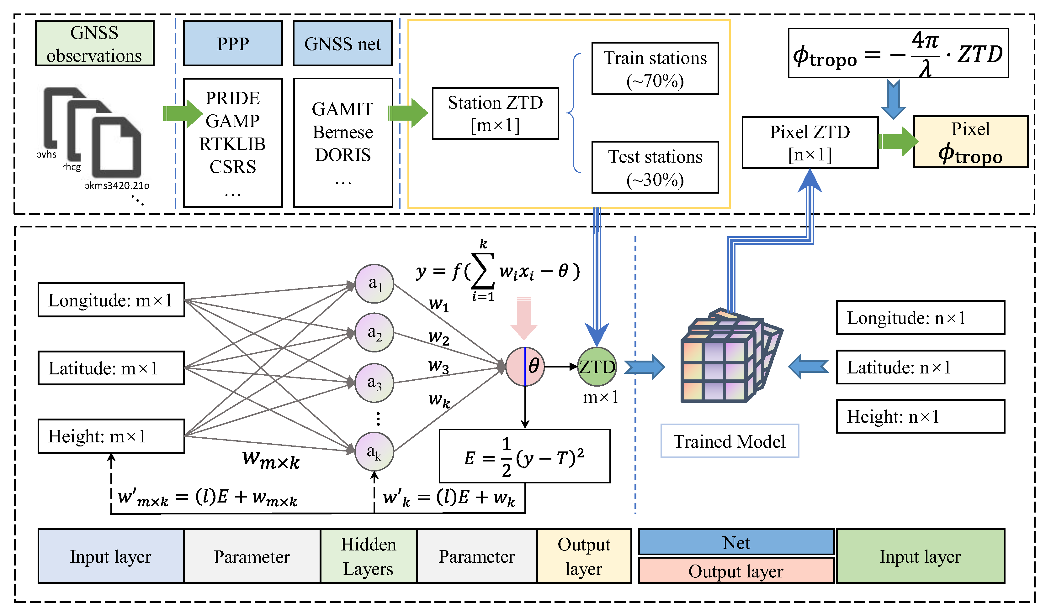
3.2.2. BP + GNSS
- Step 1: GNSS stations selection
- Step 2: Solving GNSS to obtain ZTD
- Step 3: Prediction of interferometric pixel position ZTD
- Step 4: Phase delays calculation in the LOS direction
3.2.3. ERA5
3.2.4. MERRA2
3.2.5. MODIS PWV
3.2.6. Ph-Elev (Linear)
4. Tropospheric Delays Correction Result of the Unwrapped Phases
4.1. Statistical Methods for Assessing the Quality of Corrections
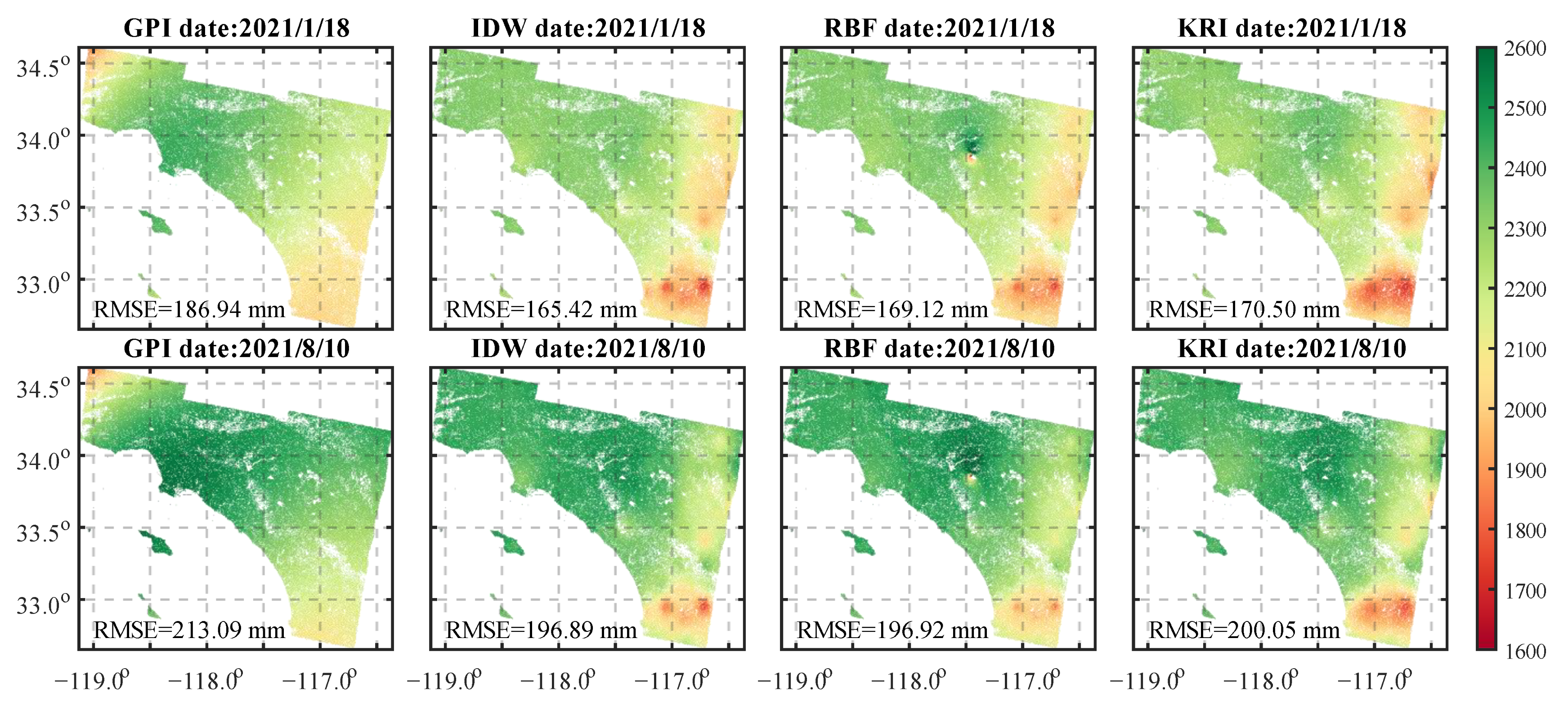
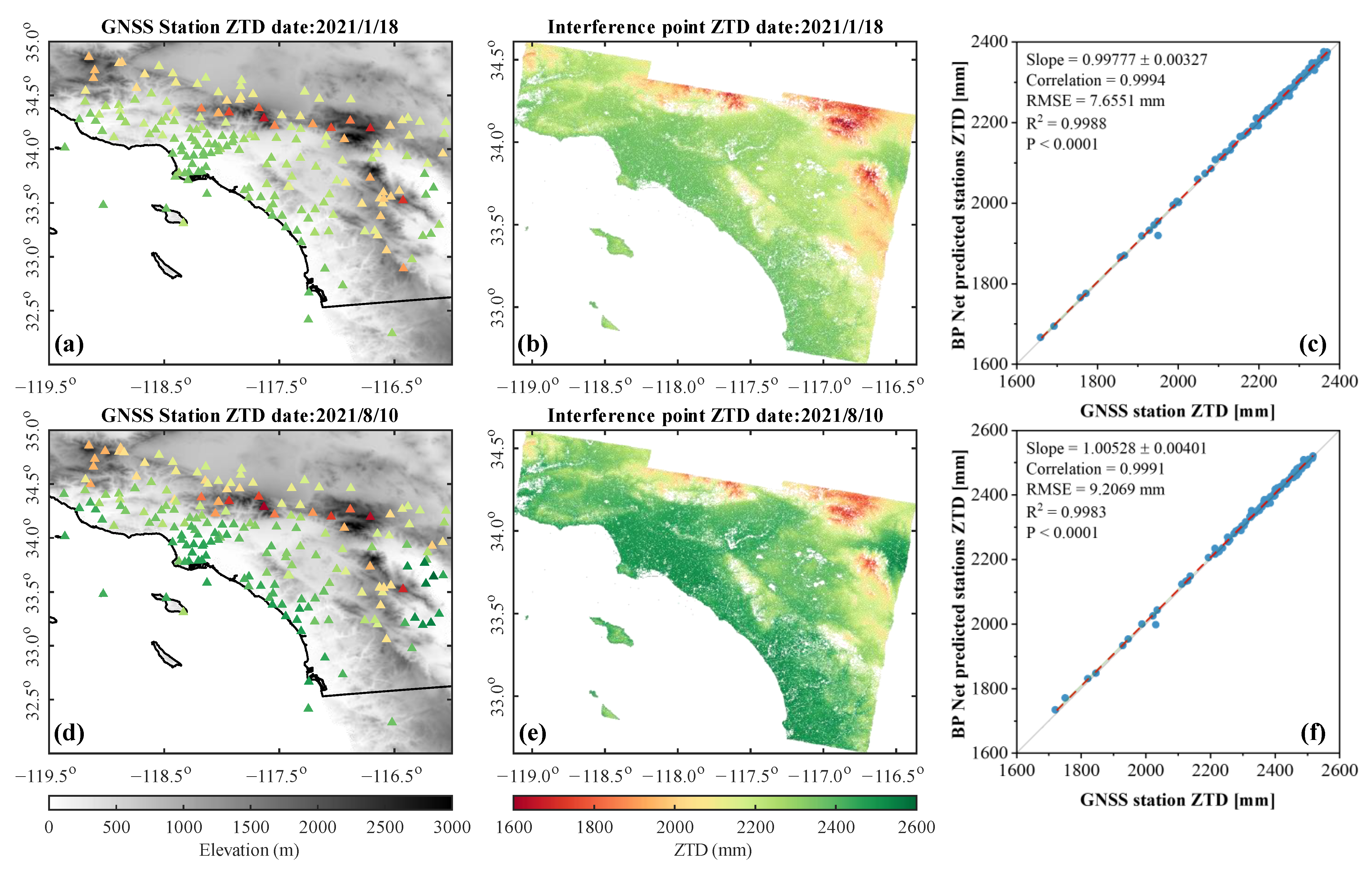
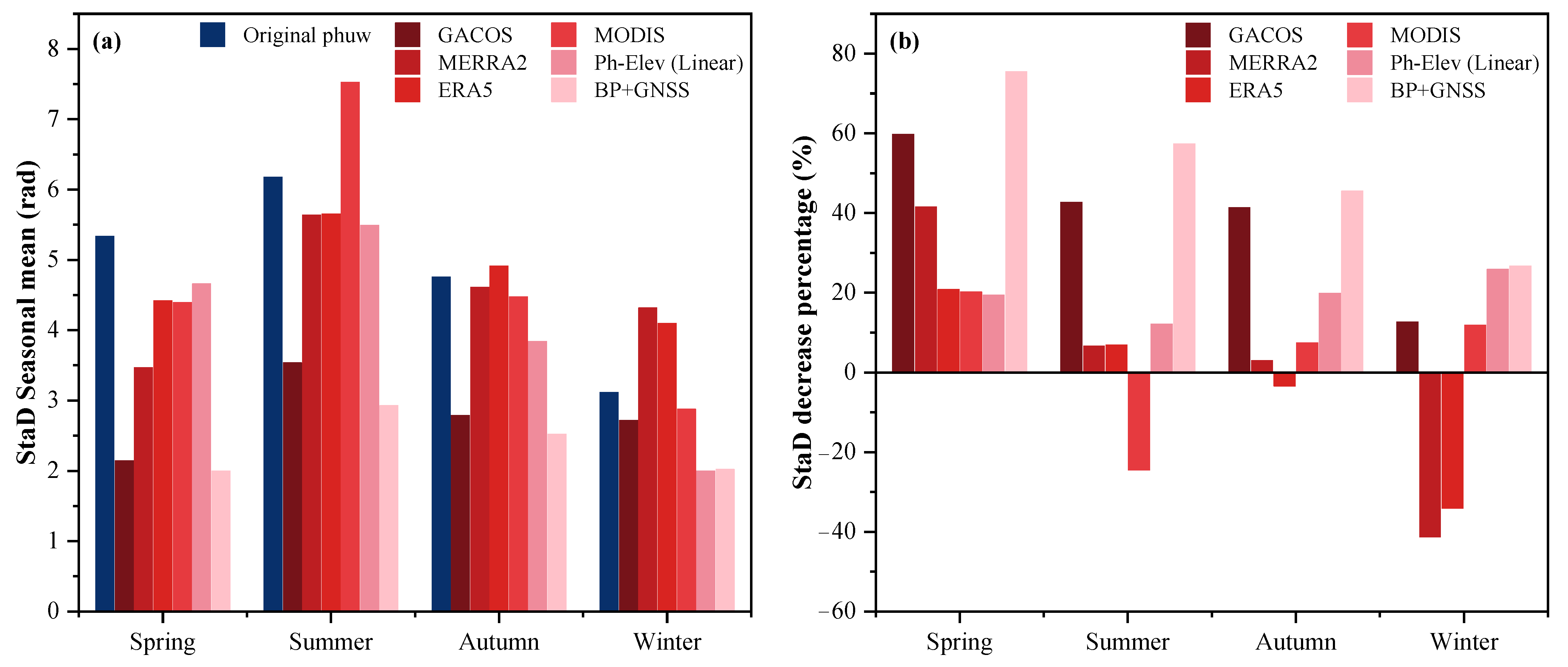
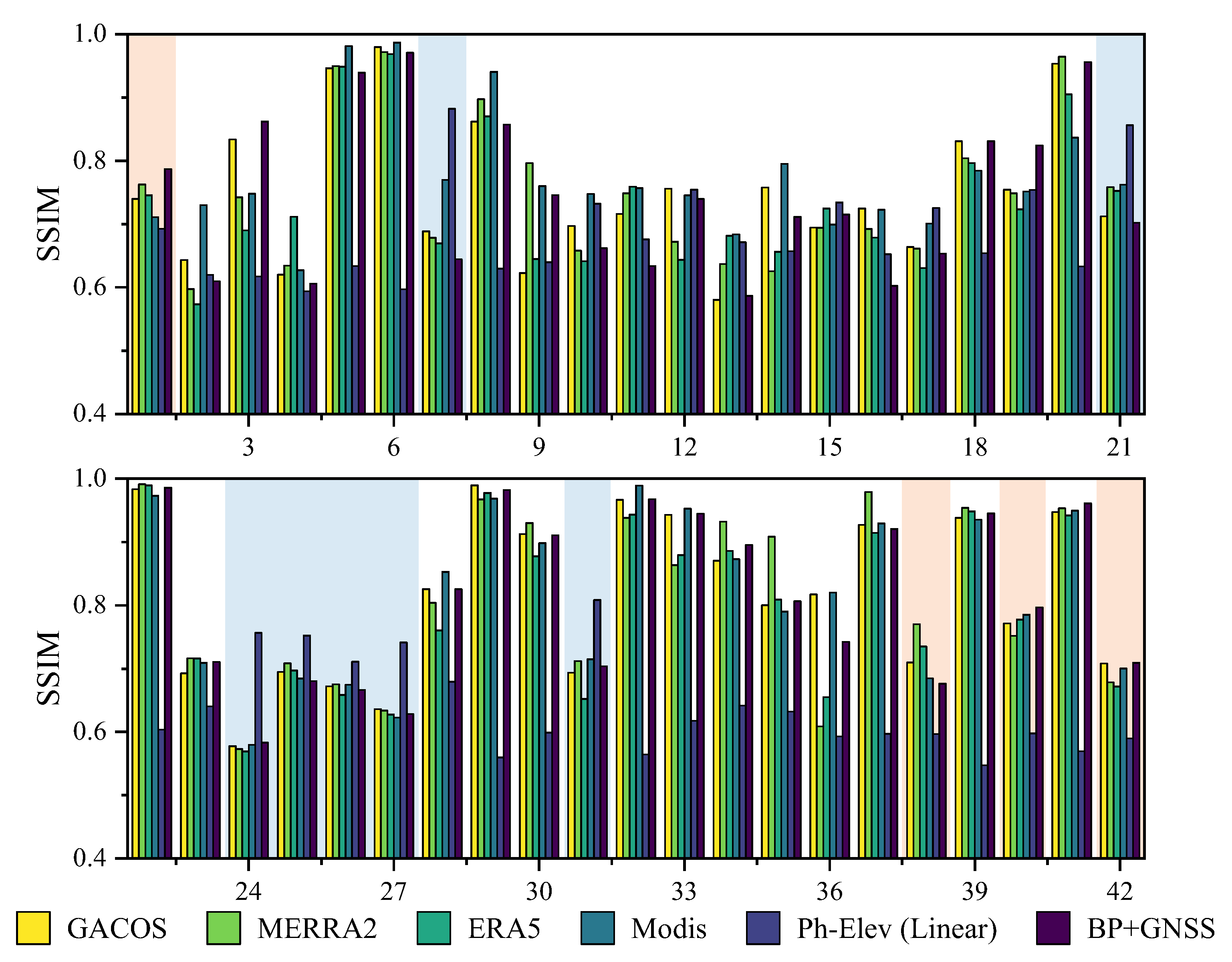
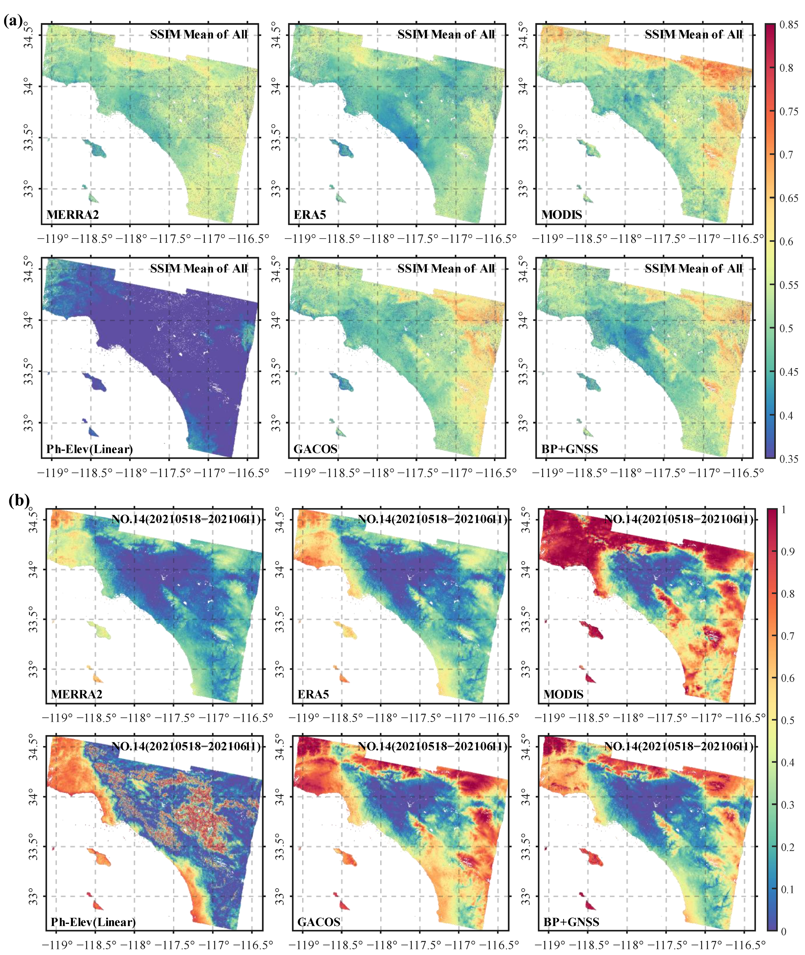
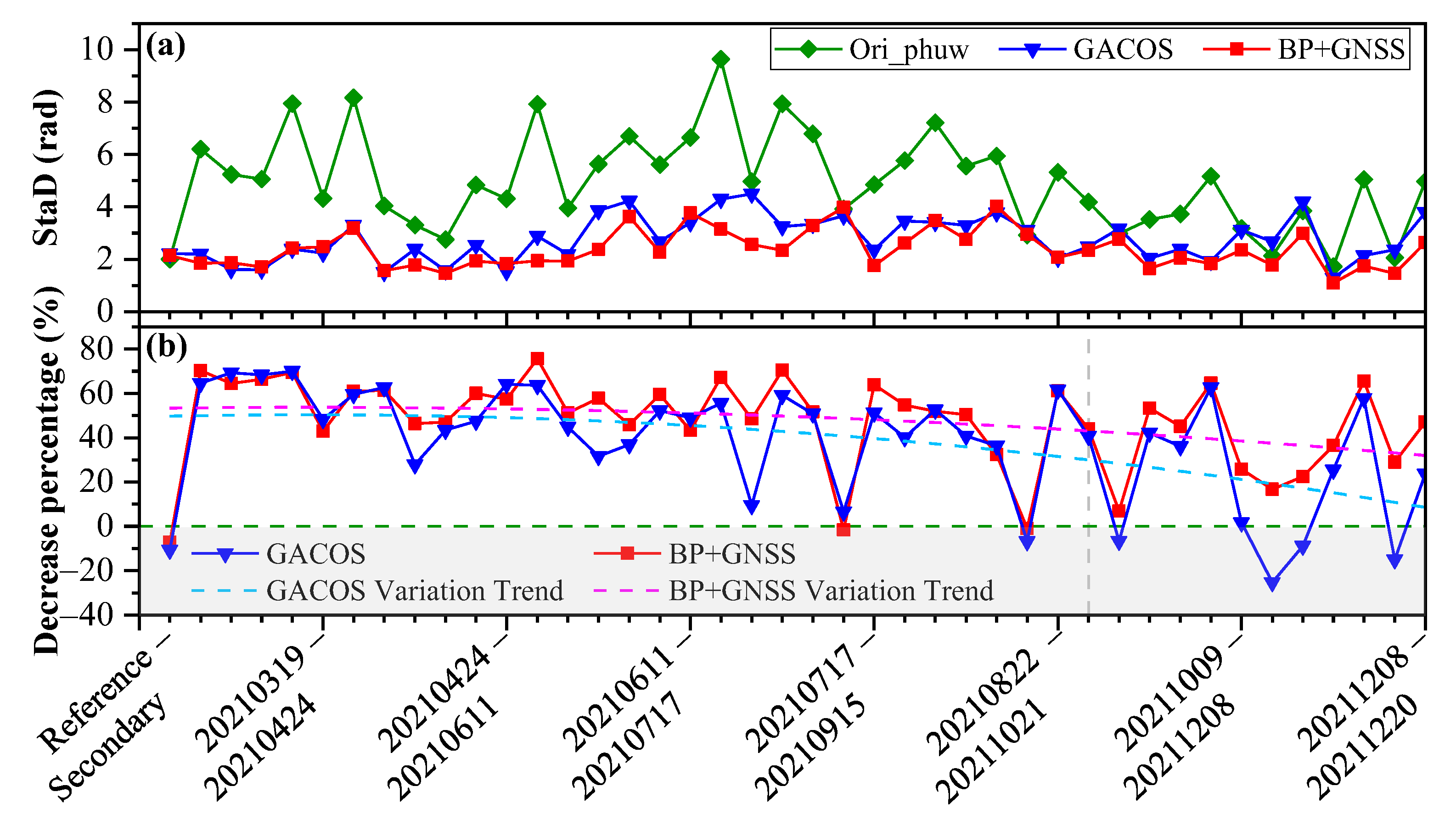
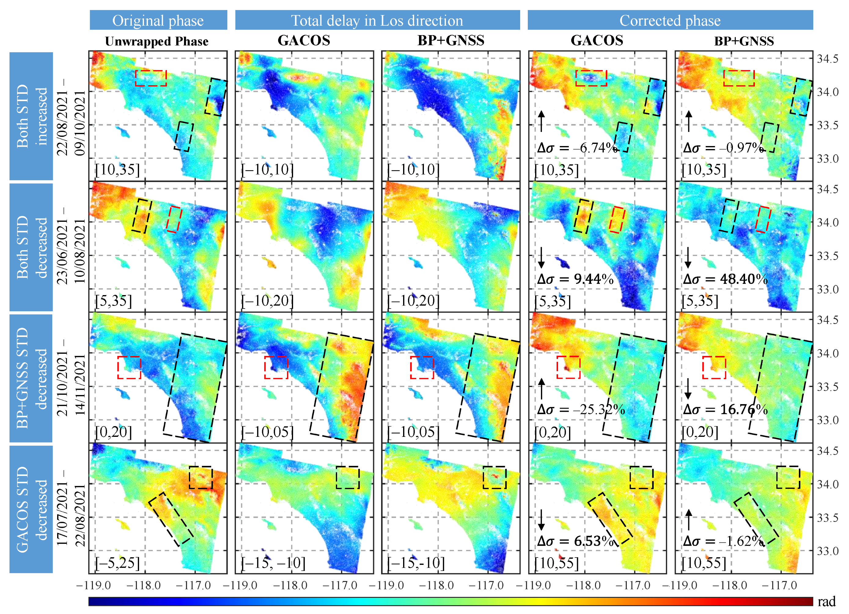
4.2. Analysis of Correction Results
5. Discussion
6. Conclusions and Outlook
Author Contributions
Funding
Data Availability Statement
Acknowledgments
Conflicts of Interest
Appendix A

| Dataset | Description | Data Product | Spatial Resolution | Coverage | Temporal Sampling | Hydrostatic Delay | Wet Delay |
|---|---|---|---|---|---|---|---|
| GNSS | Propagation delay | Zenith total delay | Station spacing | Global | 5 min | Yes | Yes-Including turbulent |
| GACOS | Operational weather model | Zenith total delay | 90 m | Global | 1 min | Yes | Yes-Including turbulent |
| ERA5 | Weather reanalysis model | Pressure; temperature; humidity | 0.25° | Global | 1 h | Yes | Yes-Including turbulent |
| MERRA2 | Weather reanalysis model | Pressure; temperature; humidity | 0.50° × 0.625° | Global | 3 h | Yes | Yes-Including turbulent |
| NARR | Weather reanalysis model | Pressure; temperature; humidity | 32 km (0.3°) | US only | 3 h | Yes | Yes-Including turbulent |
| WRF | Weather model | Pressure; temperature; humidity | adjustable | Global | adjustable | Yes | Yes-Including turbulent |
| MODIS | Spectroradiometer | Water vapor | 1 km | Global | 1–2 day | No | Yes-Including turbulent |
| MERIS | Spectrometer | Water vapor | 1.2 km | Global | 1 day (17 May 2002–4 August 2012) | No | Yes-Including turbulent |
| OLCI | Radiometer | Water vapor | 300 m | Global | 1–2 day | No | Yes-Including turbulent |
| Power–law correction | Spatially varying troposphere | Ph-Elev (Phase/DEM) | Same as the SAR data | Global | Same as the SAR data | Yes | Yes- no turbulence |
| Linear correction | Uniform troposphere | Ph-Elev (Phase/DEM) | Same as the SAR data | Global | Same as the SAR data | Yes | Yes- no turbulence |
References
- Yu, Z.; Huang, G.; Zhao, Z.; Huang, Y.; Zhang, C.; Zhang, G. A Multi-Scale Spatial Difference Approach to Estimating Topography Correlated Atmospheric Delay in Radar Interferograms. Remote Sens. 2023, 15, 2115. [Google Scholar] [CrossRef]
- Massonnet, D.; Feigl, K.L. Radar Interferometry and Its Application to Changes in the Earth’s Surface. Rev. Geophys. 1998, 36, 441–500. [Google Scholar] [CrossRef]
- Kirui, P.K.; Reinosch, E.; Isya, N.; Riedel, B.; Gerke, M. Mitigation of Atmospheric Artefacts in Multi Temporal InSAR: A Review. PFG-J. Photogramm. Remote Sens. Geoinf. Sci. 2021, 89, 251–272. [Google Scholar] [CrossRef]
- Zebker, H.A.; Goldstein, R.M. Topographic Mapping from Interferometric Synthetic Aperture Radar Observations. J. Geophys. Res. 1986, 91, 4993. [Google Scholar] [CrossRef]
- Massonnet, D.; Rossi, M.; Carmona, C.; Adragna, F.; Peltzer, G.; Feigl, K.; Rabaute, T. The Displacement Field of the Landers Earthquake Mapped by Radar Interferometry. Nature 1993, 364, 138–142. [Google Scholar] [CrossRef]
- Goldstein, R.M.; Engelhardt, H.; Kamb, B.; Frolich, R.M. Satellite Radar Interferometry for Monitoring Ice Sheet Motion: Application to an Antarctic Ice Stream. Science 1993, 262, 1525–1530. [Google Scholar] [CrossRef]
- Fruneau, B.; Achache, J.; Delacourt, C. Observation and Modelling of the Saint-Étienne-de-Tinée Landslide Using SAR Interferometry. Tectonophysics 1996, 265, 181–190. [Google Scholar] [CrossRef]
- Massonnet, D.; Thatcher, W.; Vadon, H. Detection of Postseismic Fault-Zone Collapse Following the Landers Earthquake. Nature 1996, 382, 612–616. [Google Scholar] [CrossRef]
- Tarayre, H.; Massonnet, D. Atmospheric Propagation Heterogeneities Revealed by ERS-1 Interferometry. Geophys. Res. Lett. 1996, 23, 989–992. [Google Scholar] [CrossRef]
- Williams, S.; Bock, Y.; Fang, P. Integrated Satellite Interferometry: Tropospheric Noise, GPS Estimates and Implications for Interferometric Synthetic Aperture Radar Products. J. Geophys. Res. Solid Earth 1998, 103, 27051–27067. [Google Scholar] [CrossRef]
- Simons, M.; Rosen, P.A. Interferometric Synthetic Aperture Radar Geodesy; Elsevier: Amsterdam, The Netherlands, 2007; pp. 391–446. [Google Scholar]
- Zebker, H.A.; Rosen, P.A.; Hensley, S. Atmospheric Effects in Interferometric Synthetic Aperture Radar Surface Deformation and Topographic Maps. J. Geophys. Res. Solid Earth 1997, 102, 7547–7563. [Google Scholar] [CrossRef]
- Hooper, A.; Bekaert, D.; Spaans, K.; Arıkan, M. Recent Advances in SAR Interferometry Time Series Analysis for Measuring Crustal Deformation. Tectonophysics 2012, 514–517, 1–13. [Google Scholar] [CrossRef]
- Kinoshita, Y.; Furuya, M.; Hobiger, T.; Ichikawa, R. Are Numerical Weather Model Outputs Helpful to Reduce Tropospheric Delay Signals in InSAR Data? J. Geod. 2013, 87, 267–277. [Google Scholar] [CrossRef]
- Cao, Y.; Li, Z.; Wei, J.; Hu, J.; Duan, M.; Feng, G. Stochastic Modeling for Time Series InSAR: With Emphasis on Atmospheric Effects. J. Geod. 2018, 92, 185–204. [Google Scholar] [CrossRef]
- Rosen, P.A.; Hensley, S.; Joughin, I.R.; Li, F.K.; Madsen, S.N.; Rodriguez, E.; Goldstein, R.M. Synthetic Aperture Radar Interferometry. Proc. IEEE 2000, 88, 333–382. [Google Scholar] [CrossRef]
- Chen, C.W.; Zebker, H.A. Two-Dimensional Phase Unwrapping with Use of Statistical Models for Cost Functions in Nonlinear Optimization. J. Opt. Soc. Am. A Opt. Image Sci. Vis. 2001, 18, 338–351. [Google Scholar] [CrossRef]
- Hanssen, R.F. Radar Interferometry: Data Interpretation and Error Analysis; Remote Sensing and Digital Image Processing; Springer: Dordrecht, The Netherlands, 2001; Volume 2, ISBN 978-0-7923-6945-5. [Google Scholar]
- Havazli, E.; Wdowinski, S. Detection Threshold Estimates for InSAR Time Series: A Simulation of Tropospheric Delay Approach. Sensors 2021, 21, 1124. [Google Scholar] [CrossRef]
- Cavalié, O.; Doin, M.-P.; Lasserre, C.; Briole, P. Ground Motion Measurement in the Lake Mead Area, Nevada, by Differential Synthetic Aperture Radar Interferometry Time Series Analysis: Probing the Lithosphere Rheological Structure. J. Geophys. Res. Solid Earth 2007, 112, B03403. [Google Scholar] [CrossRef]
- Lin, Y.N.; Simons, M.; Hetland, E.A.; Muse, P.; DiCaprio, C. A Multiscale Approach to Estimating Topographically Correlated Propagation Delays in Radar Interferograms. Geochem. Geophys. Geosyst. 2010, 11, Q09002. [Google Scholar] [CrossRef]
- Bekaert, D.P.S.; Hooper, A.; Wright, T.J. A Spatially Variable Power Law Tropospheric Correction Technique for InSAR Data. J. Geophys. Res. Solid Earth 2015, 120, 1345–1356. [Google Scholar] [CrossRef]
- Zhao, Y.; Zuo, X.; Li, Y.; Guo, S.; Bu, J.; Yang, Q. Evaluation of InSAR Tropospheric Delay Correction Methods in a Low-Latitude Alpine Canyon Region. Remote Sens. 2023, 15, 990. [Google Scholar] [CrossRef]
- Zhu, B.; Li, J.; Chu, Z.; Tang, W.; Wang, B.; Li, D. A Robust and Multi-Weighted Approach to Estimating Topographically Correlated Tropospheric Delays in Radar Interferograms. Sensors 2016, 16, 1078. [Google Scholar] [CrossRef] [PubMed]
- Liang, H.; Zhang, L.; Lu, Z.; Li, X. Correction of Spatially Varying Stratified Atmospheric Delays in Multitemporal InSAR. Remote Sens. Environ. 2023, 285, 113382. [Google Scholar] [CrossRef]
- Ferretti, A.; Prati, C.; Rocca, F. Permanent Scatterers in SAR Interferometry. IEEE Trans. Geosci. Remote Sens. 2001, 39, 8–20. [Google Scholar] [CrossRef]
- Hooper, A.; Segall, P.; Zebker, H. Persistent Scatterer Interferometric Synthetic Aperture Radar for Crustal Deformation Analysis, with Application to Volcán Alcedo, Galápagos. J. Geophys. Res. Solid Earth 2007, 112, B07407. [Google Scholar] [CrossRef]
- Jolivet, R.; Agram, P.S.; Lin, N.Y.; Simons, M.; Doin, M.-P.; Peltzer, G.; Li, Z. Improving InSAR Geodesy Using Global Atmospheric Models. J. Geophys. Res. Solid Earth 2014, 119, 2324–2341. [Google Scholar] [CrossRef]
- Jolivet, R.; Grandin, R.; Lasserre, C.; Doin, M.-P.; Peltzer, G. Systematic InSAR Tropospheric Phase Delay Corrections from Global Meteorological Reanalysis Data. Geophys. Res. Lett. 2011, 38, L17311. [Google Scholar] [CrossRef]
- Walters, R.J.; Parsons, B.; Wright, T.J. Constraining Crustal Velocity Fields with InSAR for Eastern Turkey: Limits to the Block-like Behavior of Eastern Anatolia. J. Geophys. Res. Solid Earth 2014, 119, 5215–5234. [Google Scholar] [CrossRef]
- Tang, W.; Yuan, P.; Liao, M.; Balz, T. Investigation of Ground Deformation in Taiyuan Basin, China from 2003 to 2010, with Atmosphere-Corrected Time Series InSAR. Remote Sens. 2018, 10, 1499. [Google Scholar] [CrossRef]
- Dong, J.; Zhang, L.; Liao, M.; Gong, J. Improved Correction of Seasonal Tropospheric Delay in InSAR Observations for Landslide Deformation Monitoring. Remote Sens. Environ. 2019, 233, 111370. [Google Scholar] [CrossRef]
- Lopez-Pozo, F.; Abarca-del-Rio, R.; Lara, L.E. ADTC-InSAR: A Tropospheric Correction Database for Andean Volcanoes. Sci. Data 2022, 9, 526. [Google Scholar] [CrossRef]
- Zhang, Z.; Lou, Y.; Zhang, W.; Wang, H.; Zhou, Y.; Bai, J. Assessment of ERA-Interim and ERA5 Reanalysis Data on Atmospheric Corrections for InSAR. Int. J. Appl. Earth Obs. Geoinf. 2022, 111, 102822. [Google Scholar] [CrossRef]
- Liu, Q.; Zeng, Q.; Zhang, Z. Evaluation of InSAR Tropospheric Correction by Using Efficient WRF Simulation with ERA5 for Initialization. Remote Sens. 2023, 15, 273. [Google Scholar] [CrossRef]
- Sailellah, S.N.; Fukushima, Y. Comparison of Tropospheric Delay Correction Methods for InSAR Analysis Using a Mesoscale Meteorological Model: A Case Study from Japan. Earth Planets Space 2023, 75, 18. [Google Scholar] [CrossRef]
- Wadge, G.; Webley, P.W.; James, I.N.; Bingley, R.; Dodson, A.; Waugh, S.; Veneboer, T.; Puglisi, G.; Mattia, M.; Baker, D.; et al. Atmospheric Models, GPS and InSAR Measurements of the Tropospheric Water Vapour Field over Mount Etna. Geophys. Res. Lett. 2002, 29, 11-1–11-14. [Google Scholar] [CrossRef]
- Liu, S.; Hanssen, R.; Mika, Á. On the Value of High-Resolution Weather Models for Atmospheric Mitigation in SAR Interferometry. In Proceedings of the 2009 IEEE International Geoscience and Remote Sensing Symposium, Cape Town, South Africa, 12–17 July 2009; Volume 2, pp. II-749–II-752. [Google Scholar]
- Jung, J.; Kim, D.; Park, S.-E. Correction of Atmospheric Phase Screen in Time Series InSAR Using WRF Model for Monitoring Volcanic Activities. IEEE Trans. Geosci. Remote Sens. 2014, 52, 2678–2689. [Google Scholar] [CrossRef]
- Dou, F.; Lv, X.; Chai, H. Mitigating Atmospheric Effects in InSAR Stacking Based on Ensemble Forecasting with a Numerical Weather Prediction Model. Remote Sens. 2021, 13, 4670. [Google Scholar] [CrossRef]
- Li, Z.; Muller, J.-P.; Cross, P.; Fielding, E.J. Interferometric Synthetic Aperture Radar (InSAR) Atmospheric Correction: GPS, Moderate Resolution Imaging Spectroradiometer (MODIS), and InSAR Integration. J. Geophys. Res. Solid Earth 2005, 110, B03410. [Google Scholar] [CrossRef]
- Li, Z.; Muller, J.-P.; Cross, P.; Albert, P.; Fischer, J.; Bennartz, R. Assessment of the Potential of MERIS Near-infrared Water Vapour Products to Correct ASAR Interferometric Measurements. Int. J. Remote Sens. 2006, 27, 349–365. [Google Scholar] [CrossRef]
- Li, Z.; Fielding, E.J.; Cross, P.; Preusker, R. Advanced InSAR Atmospheric Correction: MERIS/MODIS Combination and Stacked Water Vapour Models. Int. J. Remote Sens. 2009, 30, 3343–3363. [Google Scholar] [CrossRef]
- Li, Z.; Fielding, E.J.; Cross, P. Integration of InSAR Time-Series Analysis and Water-Vapor Correction for Mapping Postseismic Motion After the 2003 Bam (Iran) Earthquake. IEEE Trans. Geosci. Remote Sens. 2009, 47, 3220–3230. [Google Scholar] [CrossRef]
- Doin, M.-P.; Lasserre, C.; Peltzer, G.; Cavalié, O.; Doubre, C. Corrections of Stratified Tropospheric Delays in SAR Interferometry: Validation with Global Atmospheric Models. J. Appl. Geophys. 2009, 69, 35–50. [Google Scholar] [CrossRef]
- Onn, F.; Zebker, H.A. Modeling Water Vapor Using GPS with Application to Mitigating InSAR Atmospheric Distortion. Ph.D Thesis, Stanford University, Stanford, CA, USA, 2006. [Google Scholar]
- Yu, C.; Li, Z.; Penna, N.T. Interferometric Synthetic Aperture Radar Atmospheric Correction Using a GPS-Based Iterative Tropospheric Decomposition Model. Remote Sens. Environ. 2018, 204, 109–121. [Google Scholar] [CrossRef]
- Herring, T.A.; King, R.W.; Floyd, M.A.; McClusky, S.C. Introduction to GAMIT/GLOBK, Release, 10.7; Department of Earth, Atmospheric, and Planetary Sciences, Massachusetts Institute of Technology: Boston, MA, USA, 2018. [Google Scholar]
- Murray, K.D.; Bekaert, D.P.S.; Lohman, R.B. Tropospheric Corrections for InSAR: Statistical Assessments and Applications to the Central United States and Mexico. Remote Sens. Environ. 2019, 232, 111326. [Google Scholar] [CrossRef]
- Shamshiri, R.; Motagh, M.; Nahavandchi, H.; Haghshenas Haghighi, M.; Hoseini, M. Improving Tropospheric Corrections on Large-Scale Sentinel-1 Interferograms Using a Machine Learning Approach for Integration with GNSS-Derived Zenith Total Delay (ZTD). Remote Sens. Environ. 2020, 239, 111608. [Google Scholar] [CrossRef]
- Onn, F.; Zebker, H.A. Correction for Interferometric Synthetic Aperture Radar Atmospheric Phase Artifacts Using Time Series of Zenith Wet Delay Observations from a GPS Network. J. Geophys. Res. 2006, 111, B09102. [Google Scholar] [CrossRef]
- Neely, W.R.; Borsa, A.A.; Silverii, F. GInSAR: A cGPS Correction for Enhanced InSAR Time Series. IEEE Trans. Geosci. Remote Sens. 2020, 58, 136–146. [Google Scholar] [CrossRef]
- Berrada Baby, H.; Golé, P.; Lavergnat, J. A Model for the Tropospheric Excess Path Length of Radio Waves from Surface Meteorological Measurements. Radio. Sci. 1988, 23, 1023–1038. [Google Scholar] [CrossRef]
- Yu, C.; Penna, N.T.; Li, Z. Generation of Real-time Mode High-resolution Water Vapor Fields from GPS Observations. J. Geophys. Res. Atmos. 2017, 122, 2008–2025. [Google Scholar] [CrossRef]
- Bean, B.R.; Dutton, E.J. Radio Meteorology; Superintendent of Documents, US Government Print Office: Washington, DC, USA, 1966. [Google Scholar]
- Davis, J.L.; Herring, T.A.; Shapiro, I.I.; Rogers, A.E.E.; Elgered, G. Geodesy by Radio Interferometry: Effects of Atmospheric Modeling Errors on Estimates of Baseline Length. Radio. Sci. 1985, 20, 1593–1607. [Google Scholar] [CrossRef]
- Bevis, M.; Businger, S.; Herring, T.A.; Rocken, C.; Anthes, R.A.; Ware, R.H. GPS Meteorology: Remote Sensing of Atmospheric Water Vapor Using the Global Positioning System. J. Geophys. Res. Atmos. 1992, 97, 15787–15801. [Google Scholar] [CrossRef]
- Li, Z.; Muller, J.-P.; Cross, P. Comparison of Precipitable Water Vapor Derived from Radiosonde, GPS, and Moderate-Resolution Imaging Spectroradiometer Measurements. J. Geophys. Res. Atmos. 2003, 108, 4651. [Google Scholar] [CrossRef]
- Landskron, D.; Böhm, J. VMF3/GPT3: Refined Discrete and Empirical Troposphere Mapping Functions. J. Geod. 2018, 92, 349–360. [Google Scholar] [CrossRef]
- Yao, Y.; Zhang, B.; Xu, C.; Yan, F. Improved One/Multi-Parameter Models That Consider Seasonal and Geographic Variations for Estimating Weighted Mean Temperature in Ground-Based GPS Meteorology. J. Geod. 2014, 88, 273–282. [Google Scholar] [CrossRef]
- Fruneau, B.; Sarti, F. Detection of Ground Subsidence in the City of Paris Using Radar Interferometry: Isolation of Deformation from Atmospheric Artifacts Using Correlation. Geophys. Res. Lett. 2000, 27, 3981–3984. [Google Scholar] [CrossRef]
- Remy, D.; Bonvalot, S.; Briole, P.; Murakami, M. Accurate Measurements of Tropospheric Effects in Volcanic Areas from SAR Interferometry Data: Application to Sakurajima Volcano (Japan). Earth Planet. Sci. Lett. 2003, 213, 299–310. [Google Scholar] [CrossRef]
- Koulali, A.; Ouazar, D.; Bock, O.; Fadil, A. Study of Seasonal-Scale Atmospheric Water Cycle with Ground-Based GPS Receivers, Radiosondes and NWP Models over Morocco. Atmos. Res. 2012, 104–105, 273–291. [Google Scholar] [CrossRef]
- Rosen, P.A.; Gurrola, E.; Sacco, G.F.; Zebker, H. The InSAR Scientific Computing Environment. In Proceedings of the EUSAR 2012 9th European Conference on Synthetic Aperture Radar, Nuremberg, Germany, 23–26 April 2012; pp. 730–733. [Google Scholar]
- Fattahi, H.; Agram, P.; Simons, M. A Network-Based Enhanced Spectral Diversity Approach for TOPS Time-Series Analysis. IEEE Trans. Geosci. Remote Sens. 2017, 55, 777–786. [Google Scholar] [CrossRef]
- Bekaert, D.P.S.; Walters, R.J.; Wright, T.J.; Hooper, A.J.; Parker, D.J. Statistical Comparison of InSAR Tropospheric Correction Techniques. Remote Sens. Environ. 2015, 170, 40–47. [Google Scholar] [CrossRef]
- Shen, L.; Hooper, A.; Elliott, J. A Spatially Varying Scaling Method for InSAR Tropospheric Corrections Using a High-Resolution Weather Model. J. Geophys. Res. Solid Earth 2019, 124, 4051–4068. [Google Scholar] [CrossRef]
| R Squared between Height and ZTD | ZTD RMSE between GNSS and BP + GNSS | ||||||
|---|---|---|---|---|---|---|---|
| Date (dd/mm/yyyy) | R2 | Date (dd/mm/yyyy) | R2 | Date (dd/mm/yyyy) | RMSE (mm) | Date (dd/mm/yyyy) | RMSE (mm) |
| 18/01/2021 | 0.997 | 10/08/2021 | 0.970 | 18/01/2021 | 7.656 | 10/08/2021 | 9.207 |
| 23/02/2021 | 0.997 | 22/08/2021 | 0.990 | 23/02/2021 | 7.729 | 22/08/2021 | 7.716 |
| 19/03/2021 | 0.988 | 15/09/2021 | 0.991 | 19/03/2021 | 8.491 | 15/09/2021 | 7.771 |
| 12/04/2021 | 0.991 | 09/10/2021 | 0.991 | 12/04/2021 | 7.492 | 09/10/2021 | 7.569 |
| 24/04/2021 | 0.993 | 21/10/2021 | 0.994 | 24/04/2021 | 7.644 | 21/10/2021 | 6.779 |
| 18/05/2021 | 0.988 | 14/11/2021 | 0.997 | 18/05/2021 | 8.559 | 14/11/2021 | 7.566 |
| 11/06/2021 | 0.993 | 08/12/2021 | 0.994 | 11/06/2021 | 8.376 | 08/12/2021 | 7.386 |
| 23/06/2021 | 0.966 | 20/12/2021 | 0.995 | 23/06/2021 | 8.397 | 20/12/2021 | 7.549 |
| 17/07/2021 | 0.990 | - | - | 17/07/2021 | 9.241 | - | - |
| Original Unwrapped Phase | Ph-Elev (Linear) | ERA5 | MODIS | MERRA2 | GACOS | BP + GNSS | |
|---|---|---|---|---|---|---|---|
| Mean of StaD (rad) | 4.95 | 4.12 | 4.80 | 4.88 | 4.48 | 2.78 | 2.38 |
| Mean of SDP 1 (%) | - | 16.81 | 3.15 | 1.52 | 9.58 | 44.04 | 52.03 |
| NISD 2 | 42 (all) | 42 | 17 | 25 | 21 | 36 | 39 |
| CPIN 3 (%) | - | 100.00 | 40.48 | 59.52 | 50.00 | 85.71 | 92.86 |
| Mean of SSIM | - | 0.66 | 0.77 | 0.79 | 0.78 | 0.79 | 0.78 |
Disclaimer/Publisher’s Note: The statements, opinions and data contained in all publications are solely those of the individual author(s) and contributor(s) and not of MDPI and/or the editor(s). MDPI and/or the editor(s) disclaim responsibility for any injury to people or property resulting from any ideas, methods, instructions or products referred to in the content. |
© 2023 by the authors. Licensee MDPI, Basel, Switzerland. This article is an open access article distributed under the terms and conditions of the Creative Commons Attribution (CC BY) license (https://creativecommons.org/licenses/by/4.0/).
Share and Cite
Qiu, L.; Chen, P.; Yao, Y.; Chen, H.; Tang, F.; Xiong, M. An Interferometric Synthetic Aperture Radar Tropospheric Delay Correction Method Based on a Global Navigation Satellite System and a Backpropagation Neural Network: More Suitable for Areas with Obvious Terrain Changes. Sensors 2023, 23, 9760. https://doi.org/10.3390/s23249760
Qiu L, Chen P, Yao Y, Chen H, Tang F, Xiong M. An Interferometric Synthetic Aperture Radar Tropospheric Delay Correction Method Based on a Global Navigation Satellite System and a Backpropagation Neural Network: More Suitable for Areas with Obvious Terrain Changes. Sensors. 2023; 23(24):9760. https://doi.org/10.3390/s23249760
Chicago/Turabian StyleQiu, Liangcai, Peng Chen, Yibin Yao, Hao Chen, Fucai Tang, and Mingzhu Xiong. 2023. "An Interferometric Synthetic Aperture Radar Tropospheric Delay Correction Method Based on a Global Navigation Satellite System and a Backpropagation Neural Network: More Suitable for Areas with Obvious Terrain Changes" Sensors 23, no. 24: 9760. https://doi.org/10.3390/s23249760
APA StyleQiu, L., Chen, P., Yao, Y., Chen, H., Tang, F., & Xiong, M. (2023). An Interferometric Synthetic Aperture Radar Tropospheric Delay Correction Method Based on a Global Navigation Satellite System and a Backpropagation Neural Network: More Suitable for Areas with Obvious Terrain Changes. Sensors, 23(24), 9760. https://doi.org/10.3390/s23249760