1. Introduction
There has been increasing demand for multiple robotic manipulator systems (MRMSs) employed in modern manufacturing processes, such as assembling, transporting, painting, welding, and so on [
1,
2,
3,
4]. These applications require great manipulability and maneuverability; most of them cannot be achieved using a single robotic manipulator subsystem. In these situations, the utilization of multiple robotic manipulator systems is an effective choice [
5,
6,
7,
8,
9,
10].
From the perspective of a composition system, the MRMS with uncertainties can be considered a composition system with a robotic manipulator subsystem (RMS) and a communication strength subsystem (CSS), and both subsystems are coupled to each other. It is worth noting that the existing studies on MRMSs mainly focus on synchronization and consensus [
11,
12,
13,
14,
15] for the RMS, while the communication strength between robotic manipulators plays only a secondary role. For example, in the work [
12], Sun proposed adaptive controllers and a parameter estimator employing coupling control to achieve the position synchronization of multiple motion axes. In the work [
16], a distributed synchronization control scheme was proposed for a group of MRMSs with model uncertainties subject to time-varying communication delays. In the work [
17], a T-S(Takagi–Sugeno) adaptive tracking algorithm control based on the small gain theorem was proposed for an uncertain MRMS. In the work [
18], a novel adaptive control scheme for an MRMS with a time-varying parameter was proposed based on the radial basis function neural network. From the perspective of the composition system, the dynamical behavior of an RMS can be affected by the dynamical behavior of a CSS in the MRMS, and vice versa. However, in the works [
11,
12,
13,
14,
15,
16,
17,
18], the communication strength between robotic manipulators was not considered as a subsystem to be studied. In other words, it has been rare to study the dynamics of a CSS that is considered a subsystem with dynamic behavior. In summary, how to design a tracking control protocol for the RMS and a coupling matrix function for the CSS while considering the uncertainties in MRMSs is an interesting and challenging issue for the position tracking of MRMSs.
Inspired by the literature [
19,
20,
21,
22], the dynamical model of an RMS is shown mathematically as the vector differential equation with the second derivative term due to using Newton’s law of motion. Furthermore, the dynamical model of a CSS is shown mathematically as the vector differential equation with outgoing communication strength characteristics. In recent years, there have been a number of studies [
20,
21,
22,
23] on complex dynamic networks in which vector differential equations have been used to model the dynamics of the outgoing links. For example, in [
21], the concept of outgoing links was introduced using the idea of ego networks, and the dynamics of the outgoing links were modeled using vector differential equations. In the RMS considered in this paper, each robotic manipulator can be regarded as a node, and the information communication between robotic manipulators can be regarded as the outgoing link. Inspired by this, vector differential equations are considered in modeling the dynamics of the CSS. To sum up, the motivation of this study is to develop a new tracking control protocol for an RMS and coupling matrix function for a CSS such that the position of an MRMS can be tracked on the desired joint position trajectory.
Compared to the literature [
12,
13,
14,
15,
16,
17,
18,
21,
22], the main contributions and innovations of this paper include the following three points.
- (i)
The dynamical model of an RMS is described using a vector differential equation with the second derivative term and interconnected term due to Newton’s law of motion; the model is more general.
- (ii)
A vector differential equation is used to model the dynamics of CSS, and there are few studies considering the variation of the strength of communication between multiple robotic manipulators in the existing literature.
- (iii)
The position tracking for an MRMS is achieved by employing the position tracking control protocol for the RMS and the coupling matrix function for the CSS designed in this paper, which has been rarely reported in existing studies.
This paper is organized as follows. In
Section 2, the dynamical models of an MRMS with an RMS and CSS are presented, and the corresponding assumptions are given. In
Section 3, the control goal of this paper is put forward, and the corresponding control protocol and the coupling matrix function are synthesized. In
Section 4, the effectiveness of the result obtained in this paper is verified via MATLAB numerical simulation for the
N continuous two-links robotic manipulator. Finally, the conclusions of this work and the future directions are discussed in
Section 5.
Notations: denotes a diagonal matrix with as diagonal elements; denotes the Euclidean norm of vector “·” or the Frobenius norm of matrix “·”; denotes an n-dimensional Euclidean space; denotes real matrices; denotes the generation of a random number with a standard normal distribution; denotes the generation of a matrix of size , where each element is a random number in the interval [0, 1].
2. Model Description and Control Design
Consider the uncertain multiple robotic manipulator systems (MRMSs) consisting of
N robotic manipulators with the second derivative term,
, denoting the communication strength of the
ith robotic manipulator pointing to the
jth robotic manipulator. If
, then the multiple robotic manipulators system is undirected, in which
denotes the communication strength of the self-link and
. The dynamical equation of the
ith robotic manipulator subsystem (RMS) is represented as follows.
where
and
denote the joint angular position vector and the velocity vector of the
ith robotic manipulator, respectively;
denotes the acceleration vector of the
ith robotic manipulator;
denotes the overall position vector of the RMS;
is the common coupling strength of the
ith RMS;
,
, and
denote the inertia matrix, the Coriolis and centrifugal torque matrix, and the gravitational force vector, respectively;
denotes the appropriate dimensioned uncertain vector of the
ith robotic manipulator; and
and
denote the designable control protocol of
ith robotic manipulator and the determined communication protocol between the RMS and the CSS, respectively, in which
is the diagonal matrix with the constants
and
is the inner coupling vector function.
Remark 1. From the perspective of the composition system [24,25,26], the determined communication protocol in Equation (1) can be described as the coupled communication strength between the ith robotic manipulator and its adjacent robotic manipulator, in which is used to describe the information communication strength of the ith robotic manipulator pointing to the jth robotic manipulator for . From the perspective of engineering applications, Equation (
1) describes the dynamics of the
ith RMS, in which
denotes the communication strength of the
ith robotic manipulator pointing to the
jth robotic manipulator. In other words, the dynamical change of
influences the position information of the
ith RMS. Inspired by the literature [
21,
22],
is dynamically changing according to the following dynamical equation.
where
,
,
, and
.
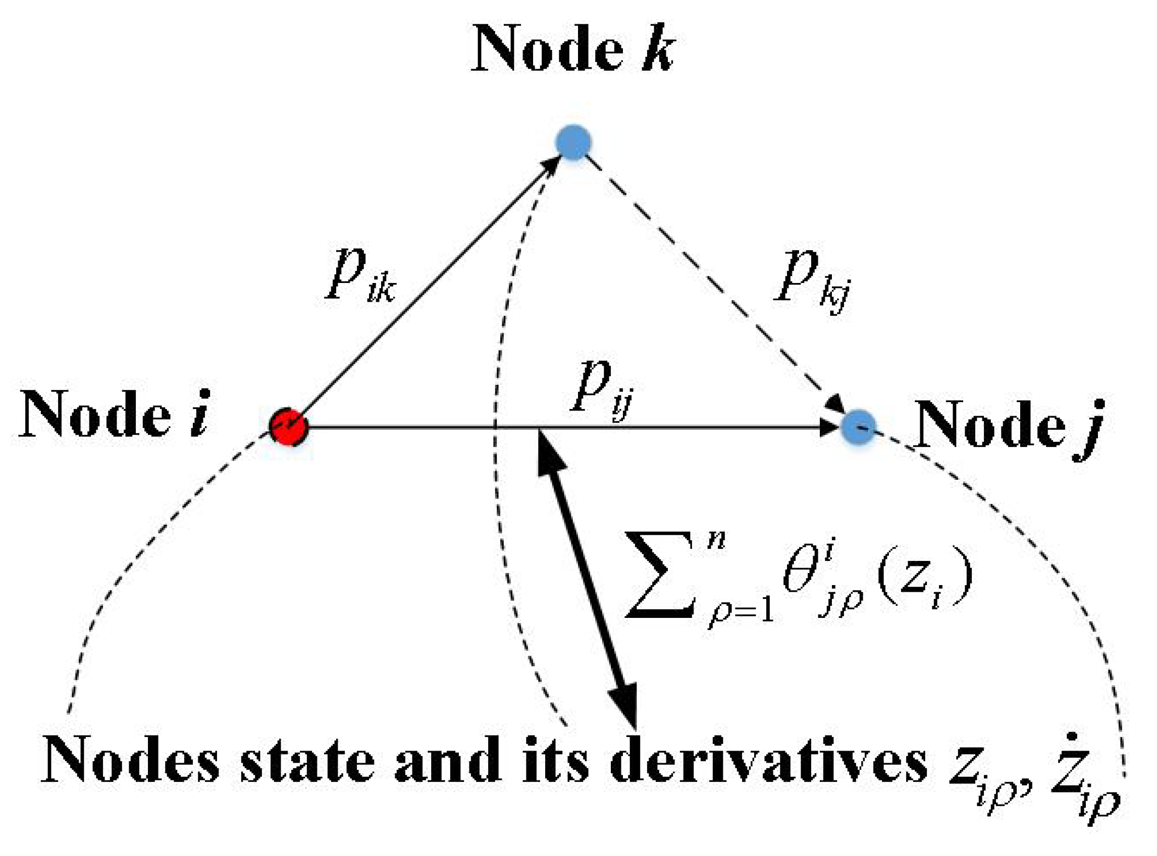
Remark 2. Equation (2) consists mainly of the linear part and the compensation part , in which and . Equation (2) can be explained graphically as follows. In
Figure 1, for a concise representation, each node denotes a robotic manipulator in the MRMS. It can be observed from
Figure 1 that the communication strength
(which denotes the communication strength of the
ith robotic manipulator pointing to the
jth robotic manipulator) is regarded as being affected directly by
(with the help of the
),
,
,
, and
. In other words, the communication strength
is regarded as the linear operation of
,
, and
for all
and
.
Definition 1 ([
21,
22]).
is called the outgoing communication strength vector for the ith robotic manipulator, respectively, . Remark 3. represents the intensity of information transmission between the ith robotic manipulator and the jth robotic manipulator, and , which is composed of all , , represents the strength of the information communication between the ith robotic manipulator and all other robotic manipulators. Then, all , consist of the communication strength subsystem (CSS).
Note that
, and then, Equation (
1) can be formulated as
Assumption 1. For Equation (3), , are known matrices, and is a known vector, in which is a symmetric, bounded invertible matrix for all . Moreover, is a known and bounded matrix, and the uncertain vector satisfies , where represents the known positive function and represents the Euclidean norm of vector or matrix. Assumption 2. For Equation (3), the position and the velocity of the ith robotic manipulator are available. Remark 4. In Equation (3), the outgoing communication strength vector denotes the overall communication strength set of the ith robotic manipulator pointing to the other robotic manipulator. In addition, Assumption 2 is mainly enlightened by some practical engineering systems. For example, in multiple robotic manipulator systems [12,13,14,15,16,27,28,29], and represent the position vector of the ith robotic manipulator and the velocity vector of the ith robotic manipulator, respectively. Their state variables, such as the angle of each joint and the speed of each joint movement, can be measured by sensors. From the perspective of the outgoing communication strength vector, Equation (
2) can be rewritten as follows.
in which
denotes the appropriate dimensioned constant matrix and
denotes the coupling matrix function between the CSS and RMS, where
.
Assumption 3. For Equation (4), the is a Hurwitz matrix for all . It is noted from Assumption 3 that all eigenvalues of
are located in the left half-plane. From the Lyapunov theory, it can be observed that there exist positive definite matrices
and
, which satisfy the following Lyapunov Equation (
5),
.
Remark 5. (i) For Equation (4), denotes the coupling matrix function between the RMS and CSS and needs to be designed. (ii) Equation (4) is largely enlightened by the literature [21,22], which represents the dynamical properties of the links relationship (communication strength) between nodes (robotic manipulators) in the complex dynamical network, where denotes the outgoing link vector (outgoing communication strength vector) of the ith node (robotic manipulator) for all . 3. The Design of Tracking Control Protocol and Coupling Matrix Function
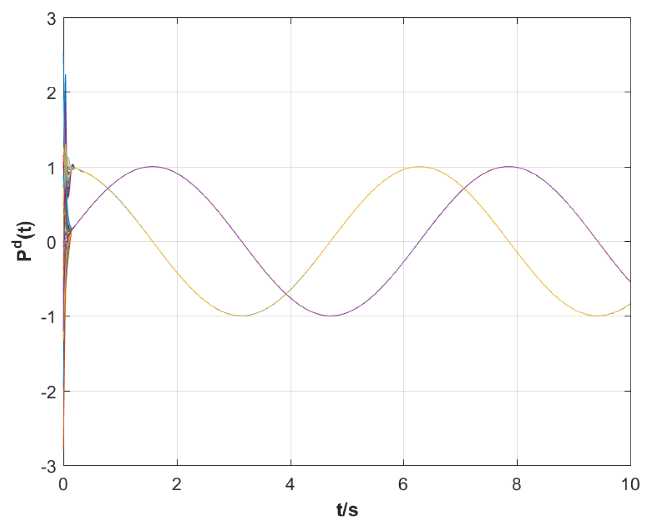
We introduce and , which are the desired joint position trajectory of the ith robotic manipulator and the desired communication strength trajectory of the ith CSS, respectively. In addition, and its derivatives , are all bounded and smooth. Note that and denote the position tracking error of the ith robotic manipulator and the communication strength error of the ith CSS, respectively, where .
Control goal. Consider the MRMS with RMS (
3) and CSS (
4). Design the control protocol
for RMS (
3) and the coupling matrix function
for CSS (
4) such that
0 holds, which means that the multiple robotic manipulator system achieves position tracking. Meanwhile, the outgoing communication strength vector
is bounded. In order to achieve the above control goal, the following control scheme is obtained.
where
denotes the
nth order identity matrix and
denotes an adjustable positive parameter, where
.
, and it is seen that
holds.
In addition, in order to assist the RMS in achieving positional tracking, an auxiliary communication strength
is introduced, and the dynamical equation of
can be described as follows
Remark 6. (i) For Equation (8), since is the positive definite matrix and is a symmetric, bounded invertible matrix, that is, the inverse of matrices and is bounded, β, σ, Γ, and are bounded. It can be concluded that the coupling matrix function is bounded, where . (ii) In Equation (9), because , , and are bounded, that is, is bounded, and is a Hurwitz matrix, it follows that the desired communication strength trajectory is bounded, where . (iii) The control protocols (6) and (7) and the coupling matrix function (8) constitute the control scheme of this paper, where the control protocols (6) and (7) are designed in the RMS and the coupling relation (8) is designed in the CSS. The combined action of these two parts makes the position of the ith robotic manipulator track along the desired joint position trajectory, while the communication strength between robotic manipulators is bounded, where . (iv) In designing the control scheme, the information that can be used is the state information of the multiple robotic manipulators, such as the position, speed, acceleration of the multiple robotic manipulators, and some information that is known in the system. It is worth noting that we cannot utilize the communication strength information because the position and speed of the robotic manipulators can be measured via suitable sensors, whereas the strength of the communication between the robotic manipulators is difficult to be accurately measured using suitable sensors. Therefore, because of cost, technical limitations, and other factors, the strength of communication between robotic manipulators cannot be accurately obtained in this paper, and consequently, the information on communication strength cannot be used in the control scheme. From
, Equations (
3), (
4) and (
9), and the control protocol (
6), the position tracking error and the communication strength error equations for the RMS (
3) and CSS (
4) can be obtained as follows:
Theorem 1. Consider the MRMS with RMS (3) and CSS (4). If Assumptions 1–3 are satisfied, the control protocols and are designed, and the coupling matrix function is synthesized; the position tracking error is asymptotically stable and the outgoing communication strength vector is bounded for all . Proof of Theorem. Consider the positive definite function
, where since
and
are positive definite matrices, it is clear that
is positive definite. To facilitate the subsequent derivation, it can be written in the vector form as follows:
Differentiating
with respect to time yields
According to Equations (
10) and (
11), Equation (
13) can be derived as
According to Equation (
5), it can be further obtained that
Then, by substituting the control protocol (
6) and the coupling matrix function (
8) into Equation (
14) and taking into consideration Assumption 1, the following expression is achieved:
□
Remark 7. From inequality (15), it can be seen that is negative semi-definite about , , and . In other words, the error systems , , and are stable; that is, , , and are bounded. By using Barbalat’s lemma [30,31,32], one can see thatthe position tracking error 0 holds and the velocity vector and the outgoing communication strength vector are bounded for all Remark 8. The following procedures for applying Theorem 1 are summarized to achieve the position tracking control for the RMSs.
Step 1. Give the desired joint position trajectory
, its derivatives
,
for RMS (
3), the desired communication strength trajectory
for CSS (
4) for all
, and their initial state values.
Step 2. Determine the known matrices , , the known vector , the common coupling strength , the diagonal matrix , the inner coupling matrix , the known positive function , and the adjustable positive parameter .
Step 3. Determine the positive definite matrices
by solving the Lyapunov Equation (
5).
Step 4. Determine the designed control protocols (
6) and (
7) and the coupling matrix function (
8) by substituting in the above parameters. At this point, Theorem 1 is realized; that is,
0 holds, and the outgoing communication strength vector
is bounded for all
.
4. Illustrative Example
In this section, we test our proposed control scheme on the position tracking control of
N two-link (
n = 2) robotic manipulators with uncertainties in [
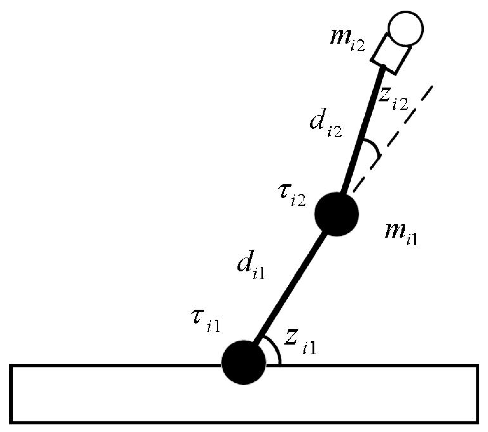
33] via simulation experiments, in which the dynamics model of each isolate robotic manipulator (see
Figure 2) in joint space can be expressed as
where
and
denote the position vector of the
ith robot arm as well as the velocity vector, respectively,
denotes the angular position of the first robot arm, and
denotes the angular position of the second robot arm. In this paper, the main consideration is the position tracking problem of the two-link robotic manipulators, so the dynamics of
is the main concern of this paper.
The internal connection relation term can be described as a given communication protocol. Inspired by the literature [
21], we consider the given communication transmission protocol as
in this paper. Then, Equation (
16) can be rewritten in the form of Equation (
1) in this paper, as follows:
In addition, the dynamics of the communication strength
,
, between the two-link robotic manipulators is shown below, which is the same as Equation (
4).
In
Figure 2,
and
denote the masses of the first arm and the second arm for the
ith robotic manipulator, respectively.
and
denote the lengths of the first arm and the second arm for the
ith robotic manipulator, respectively.
and
denote the torque on the first arm and the second arm for the
ith robotic manipulator, respectively.
and
denote the positions of the first arm and the second arm for the
ith robotic manipulator, where
.
Note that , , , and .
The numerical parameters of the
ith two-link robotic manipulator are selected according to the following steps, which are derived from the numerical simulation example in [
33].
(i) The inertia matrix
, the Coriolis and centripetal force matrix
, and the gravitational force vector
can be described as
Moreover, the uncertain function
can be described as
where
is a random number to reflect the uncertainty of the function
and
and
, respectively, in which
,
,
and
denotes the generation of a random number with a standard normal distribution.
(ii) The initial states of
and
are generated by the functions
rad and
rad in MATLAB, respectively.
denotes the generation of a matrix of size
, where each element is a random number in the interval [0, 1]. The desired joint position trajectory
are
, and the desired communication strength trajectory
is given by Equation (
9).
(iii) In order to generate the Hurwitz matrix , let be a randomly generated negative number and be a stochastically produced N-order invertible symmetric matrix in MATLAB. It can be concluded that the Hurwitz matrix .
(iv) Let
, in which
and
denotes the
N order identity matrix, which is substituted into the Lyapunov equation, Equation (
5), to obtain the positive definite matrix
,
.
In the simulations, the model parameters of the two-link robotic manipulator are
,
= 10 kg,
= 2 kg,
m,
m,
g = 9.8 m/s
2,
, and
. Finally, the model parameters and the matrices obtained from the above steps are substituted into the position tracking control protocols
(
6) and
(
7) and the coupling matrix function
(
8) designed in this paper. In addition, in order to demonstrate the advantages of the position tracking control scheme synthesized in this paper, we introduce an experiment comparing the position tracking proposed in [
33,
34,
35] with ours. For simplicity, let
be the total position tracking error of the RMS in the MRMS. The simulation results are shown in
Figure 3,
Figure 4,
Figure 5 and
Figure 6.
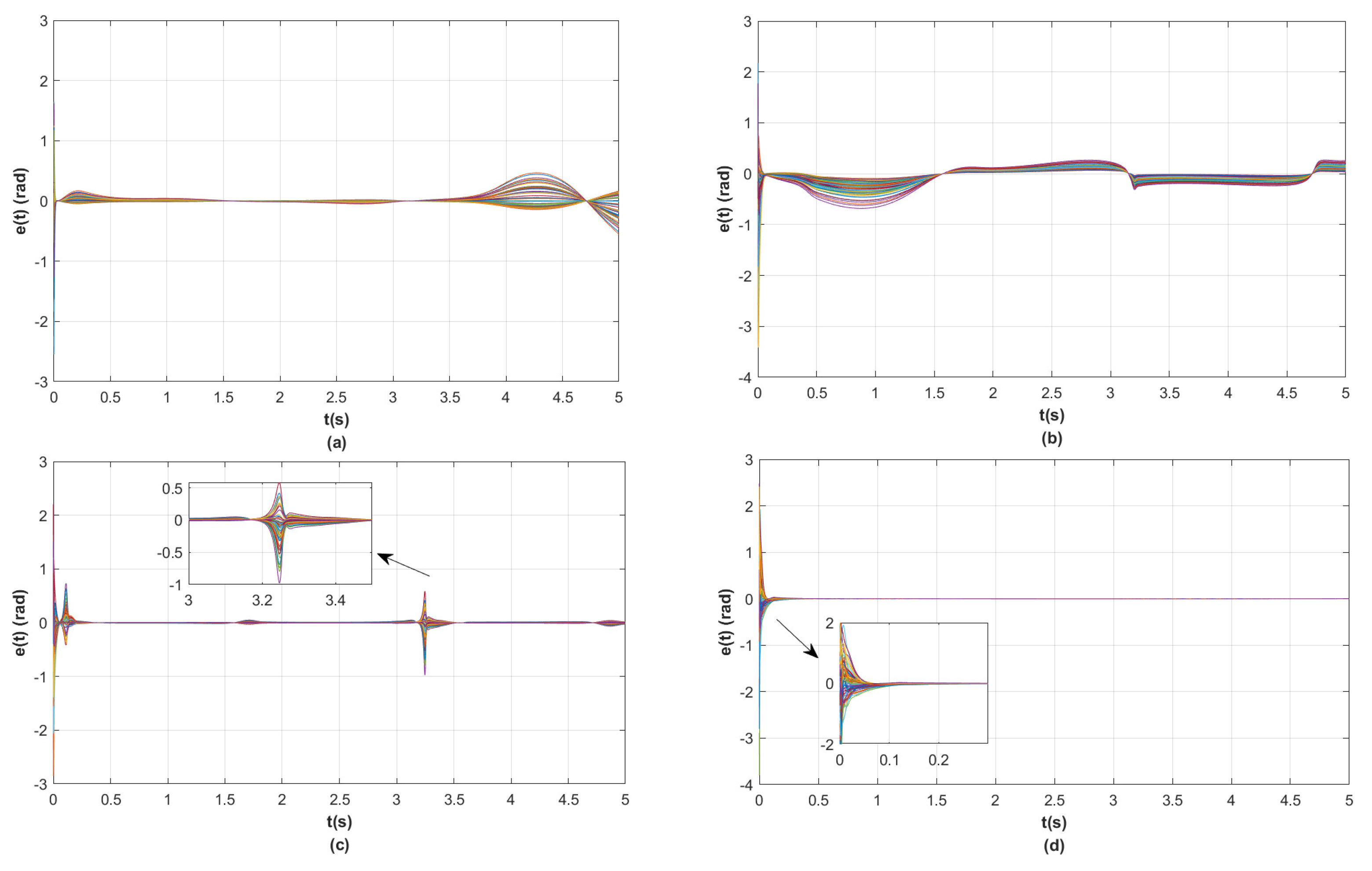
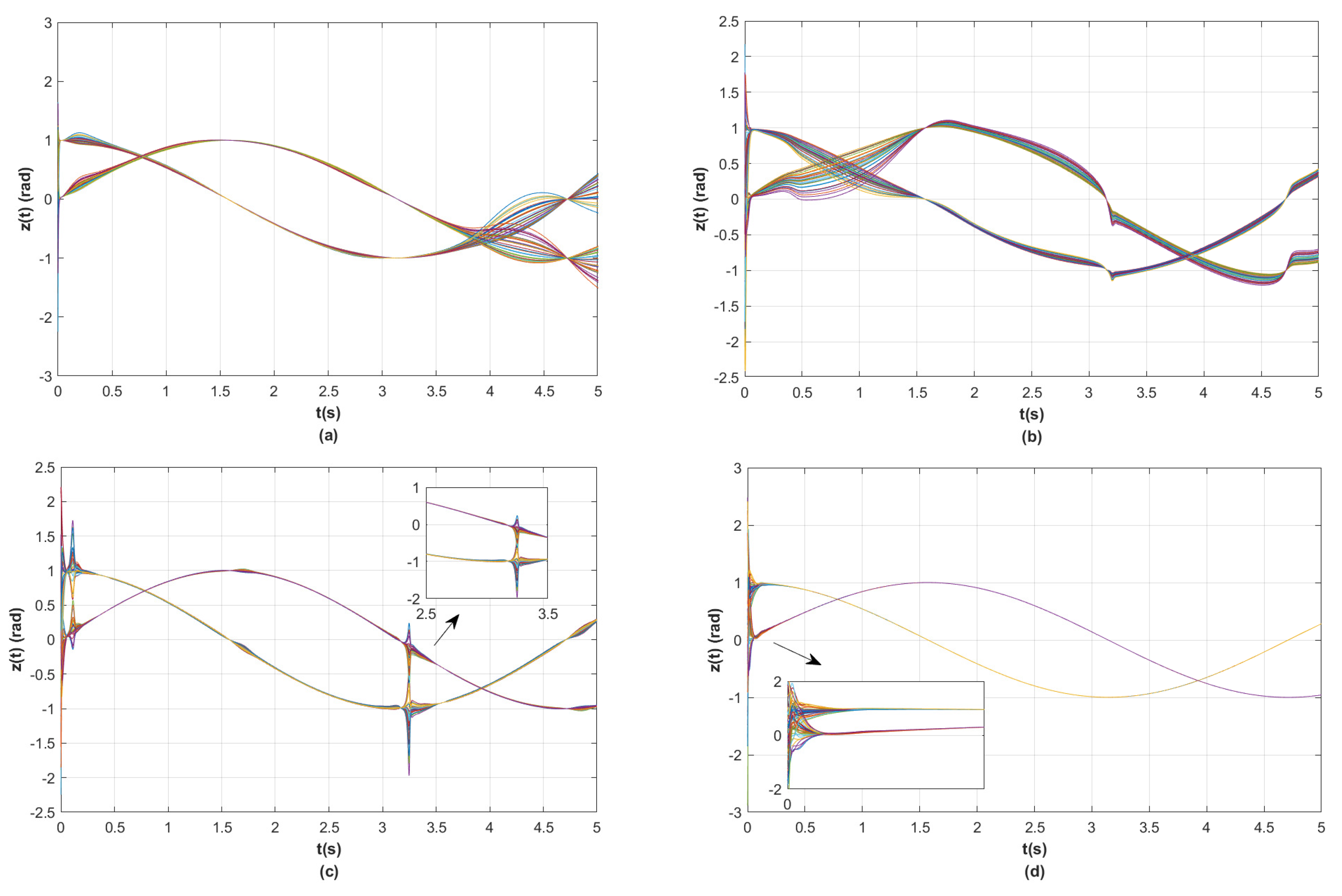
(i) As shown in
Figure 3, the differently colored curves show the state of the joint angular position of the 30 robotic manipulators. It can be seen that the control scheme in [
33,
34,
35] cannot make the joint angle positions of the RMS track the desired trajectory. That is to say, the control scheme in [
33,
34,
35] leads to larger errors of position tracking for the RMS, but the control scheme in this paper can make the position state vector of the MRMS track the desired joint position trajectory quickly.
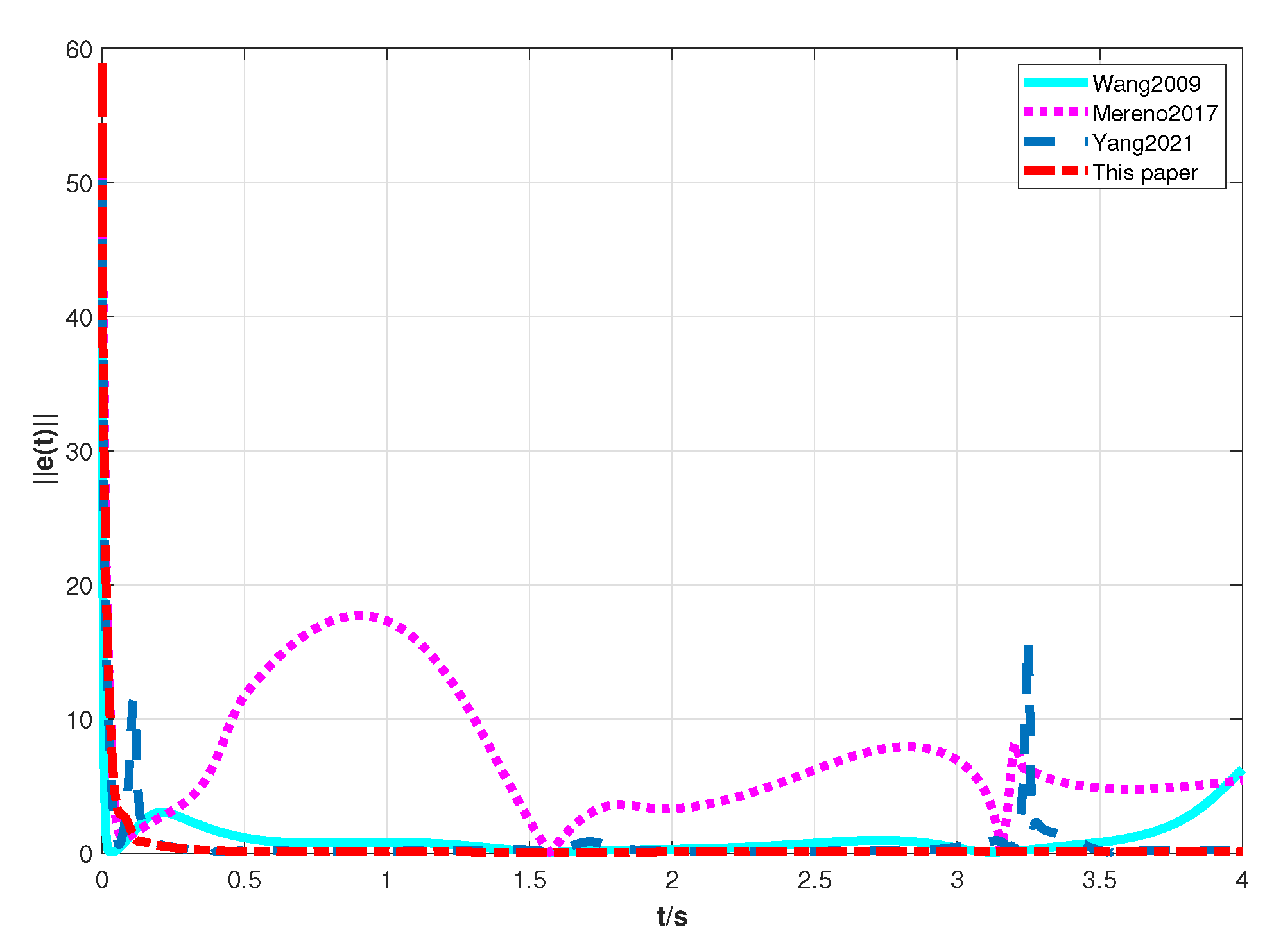
(ii)
Figure 4 and
Figure 5 illustrate that the results of the position tracking control scheme for the RMS in this paper are comparative with the ones in [
33,
34,
35]. It is clear from
Figure 4 that the position tracking control error of the RMS converges asymptotically to zero by using the control scheme in this paper. Nevertheless, the position tracking control error of the RMS does not tend to zero when employing the control scheme in [
33,
34,
35]. Moreover, the fast convergence speed of the position tracking control error of RMS in this paper is faster than the ones in [
33,
34,
35]. Above all, it can be seen that when realizing the position tracking control of the RMS, the control scheme of this paper is more appropriate than the ones in [
33,
34,
35].
(iii) It is clear from
Figure 6 that the desired communication strength trajectory
is bounded and does not converge asymptotically to zero, which means that the eventual MRMS structure is shown as all the RMSs are not isolated when the position tracking of the RMS happens.


