
Diffusion Model for DAS-VSP Data Denoising


Abstract
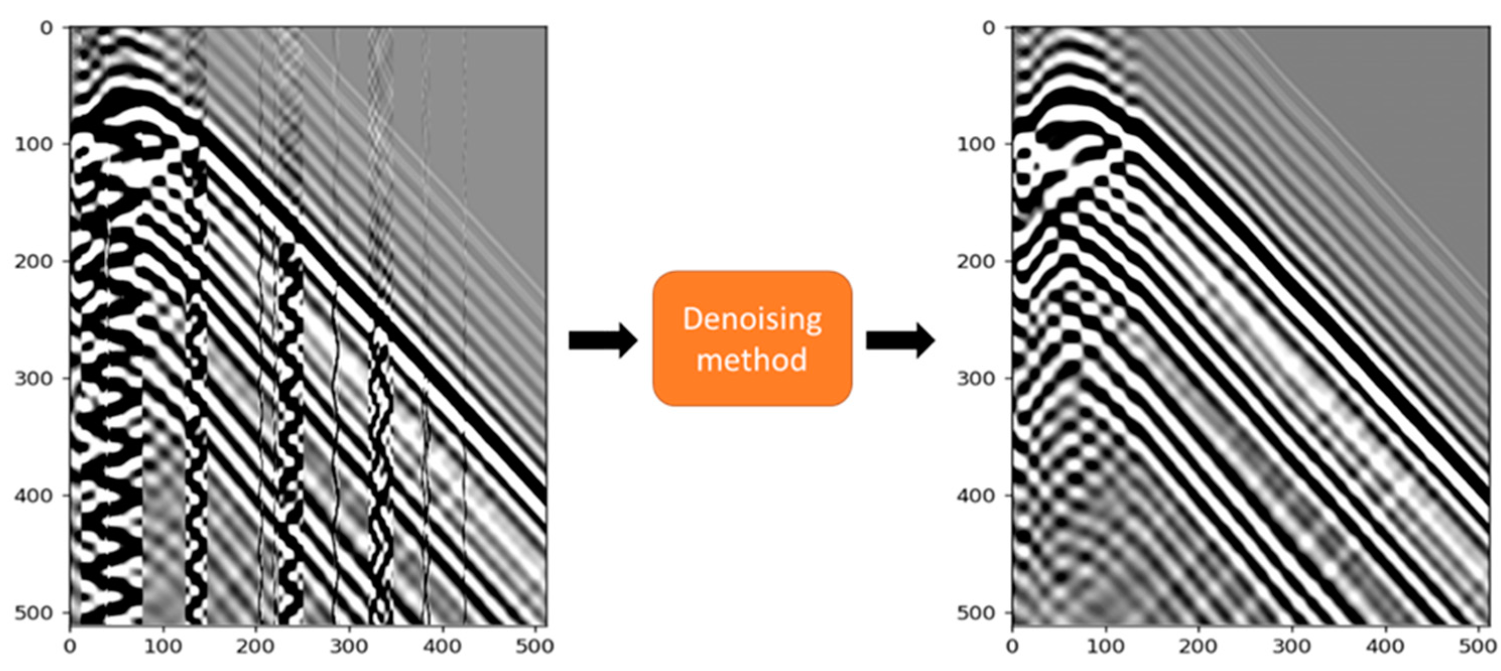
:1. Introduction
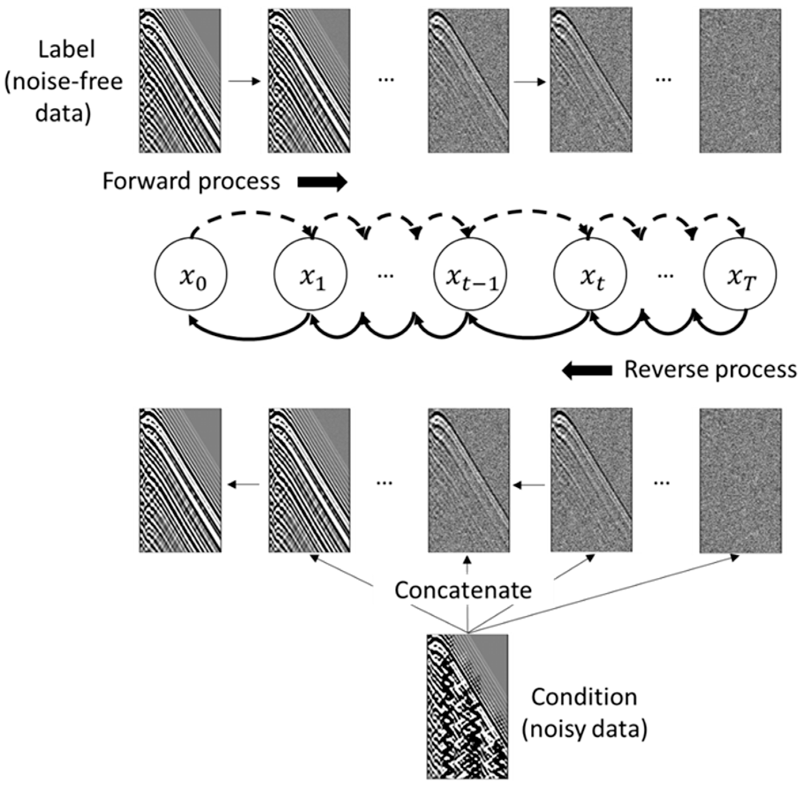
2. Methods
2.1. Forward Process
2.2. Reverse Process
2.3. Conditional Diffusion Models
2.4. Training and Loss Function
2.5. Synthetic Training Data Generation
3. Results
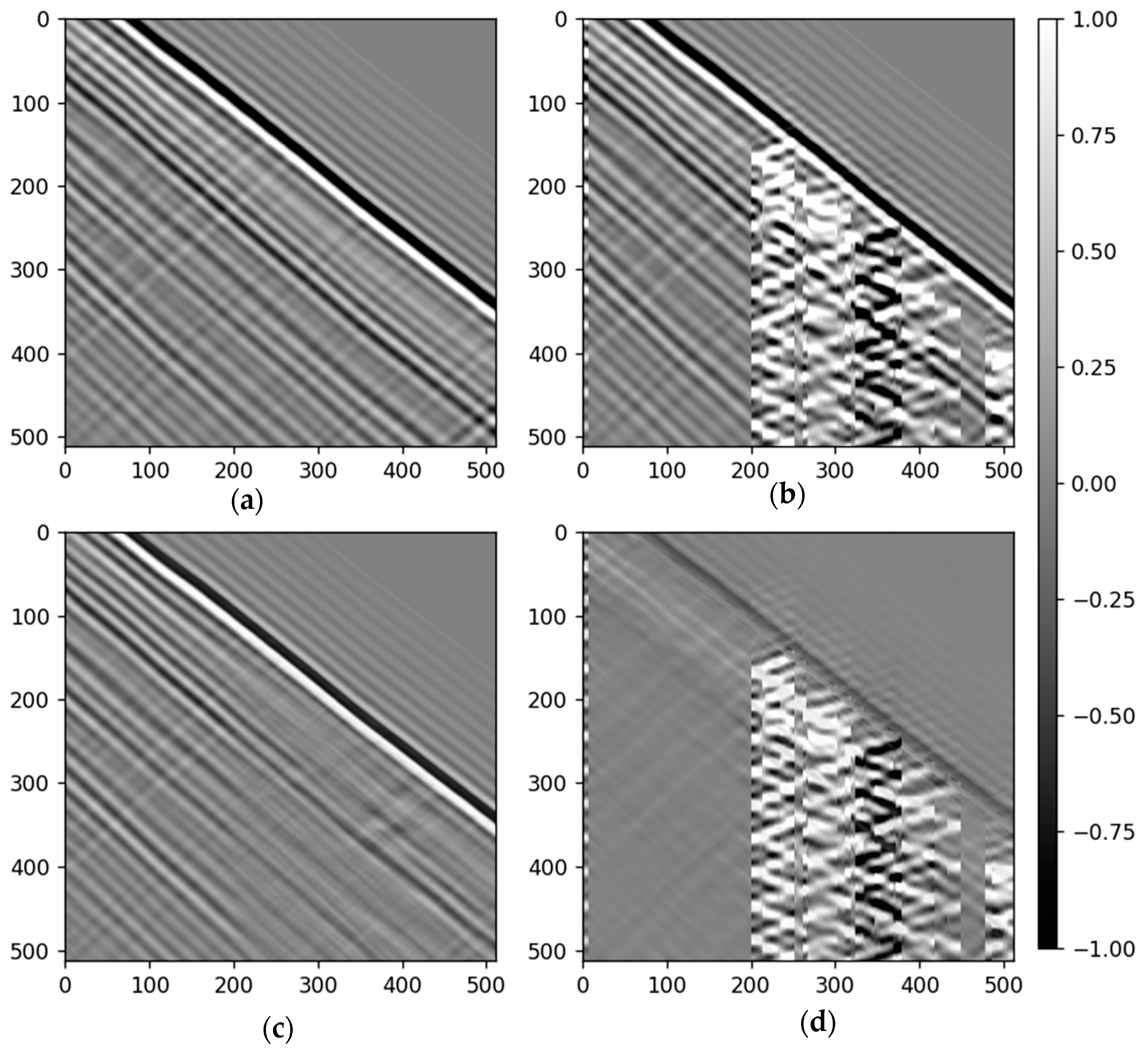
3.1. Test on the Synthetic Dataset
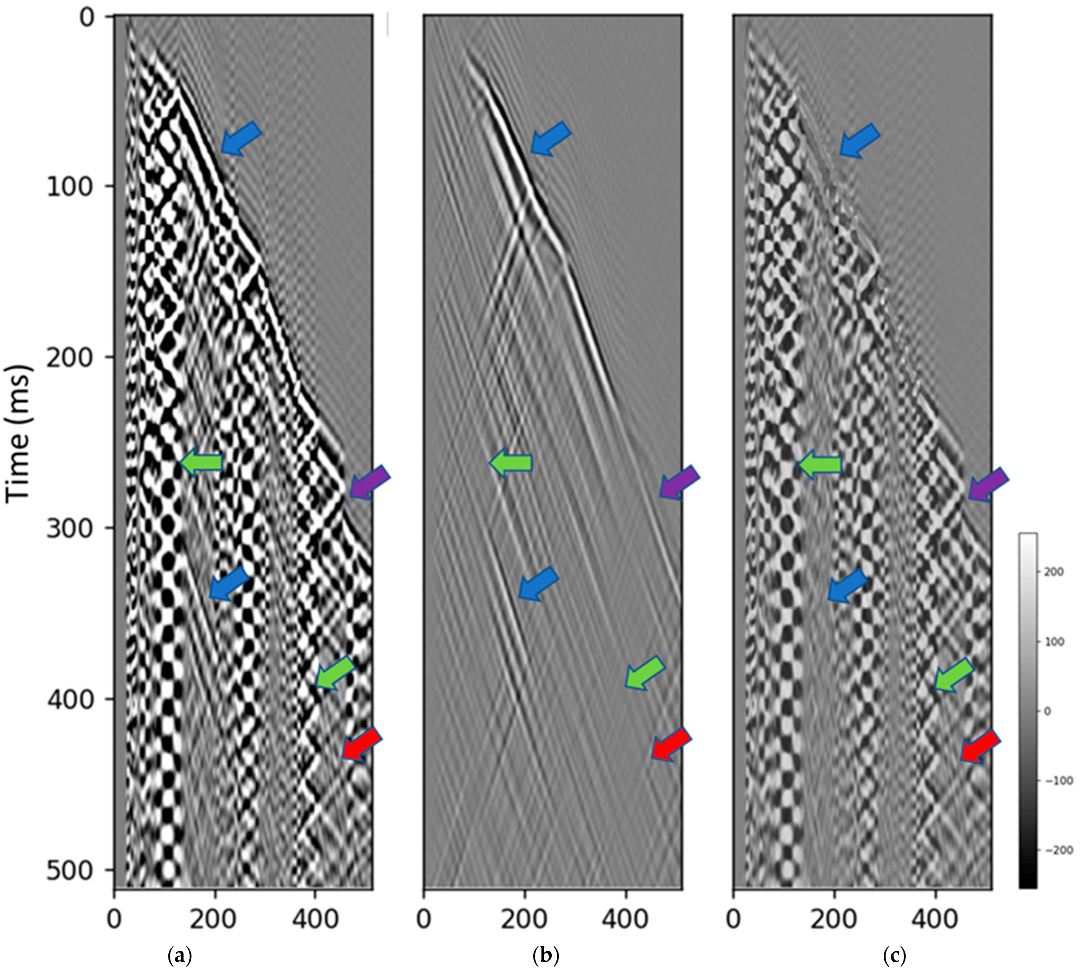
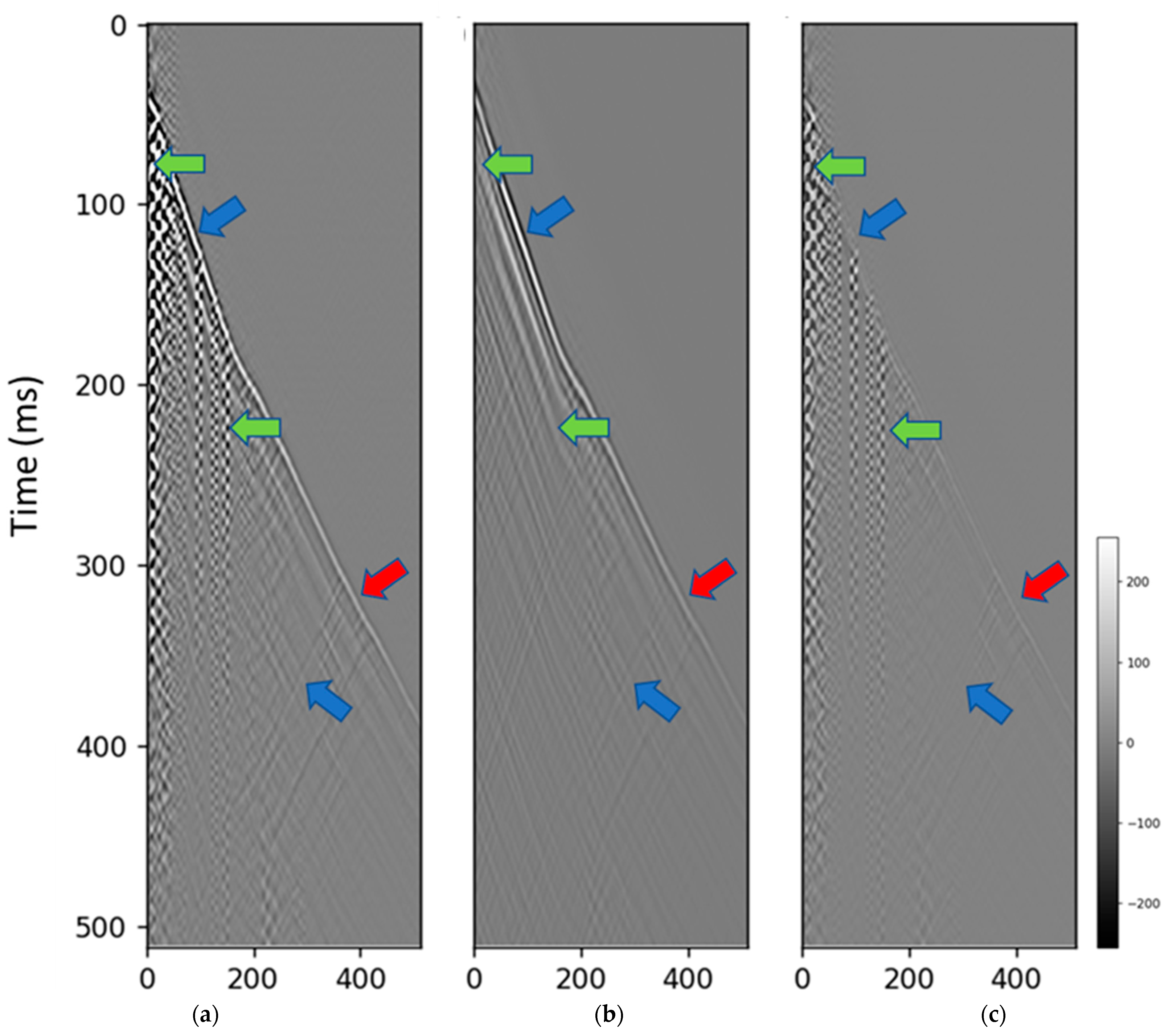
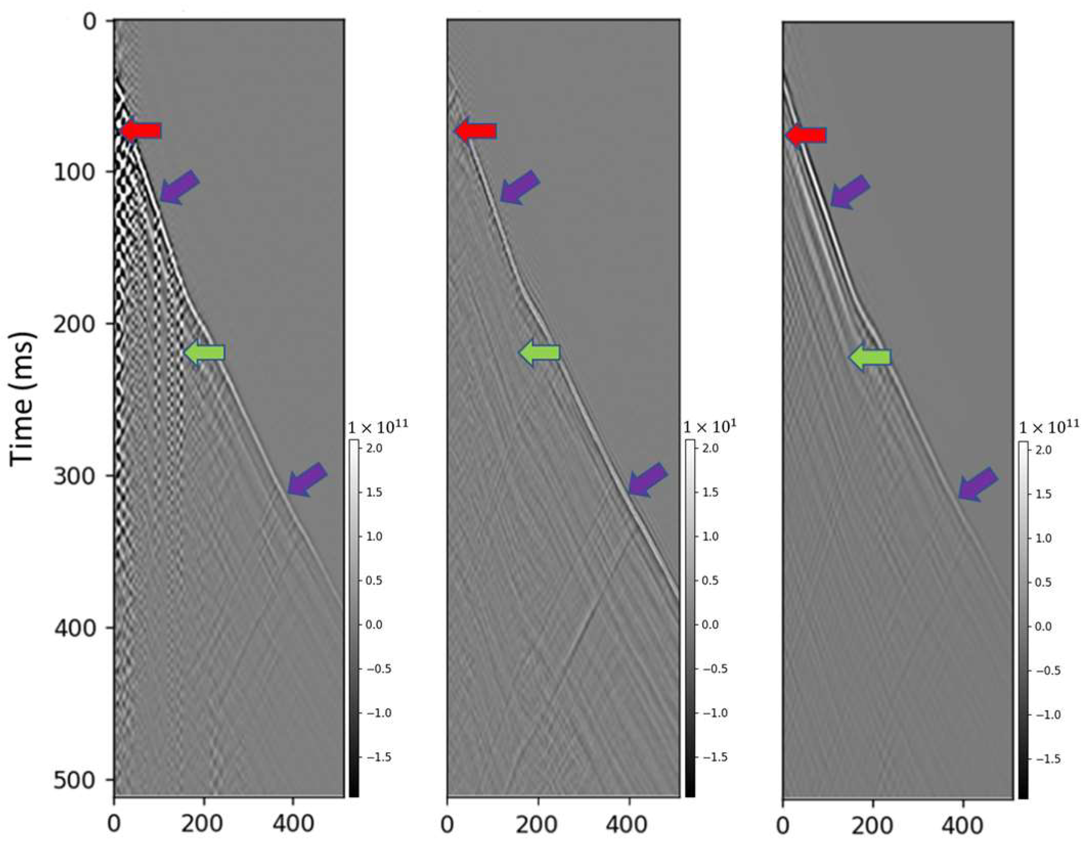
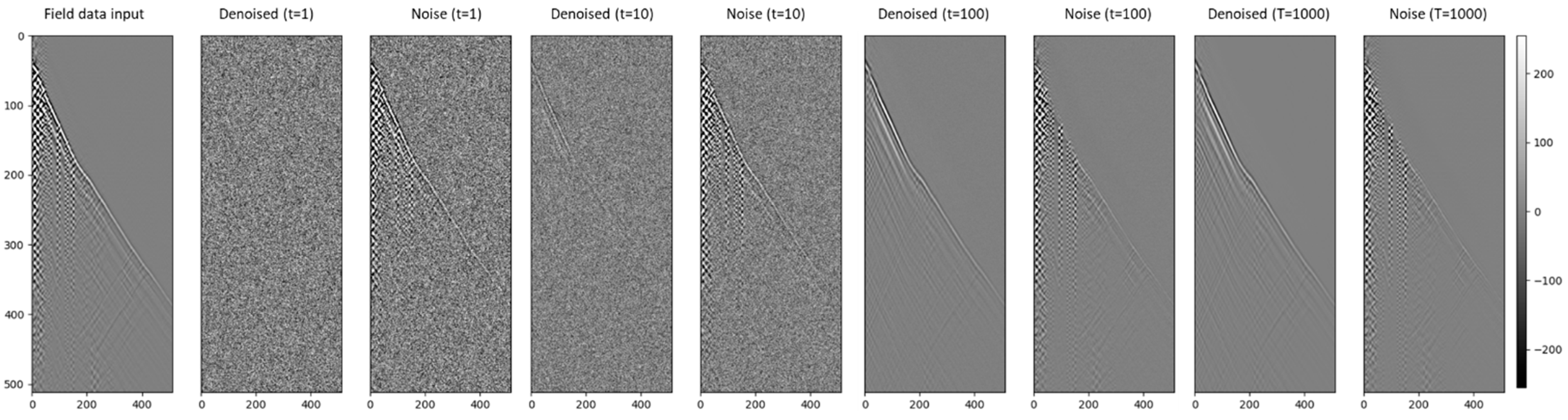
3.2. Test on the Field Data
4. Discussion
4.1. Diffusion Time-Step Analysis
4.2. Advantages and Limitations
5. Conclusions
Author Contributions
Funding
Data Availability Statement
Conflicts of Interest
References
- Mateeva, A.; Lopez, J.; Potters, H.; Mestayer, J.; Cox, B.; Kiyashchenko, D.; Wills, P.; Grandi, S.; Hornman, K.; Kuvshinov, B.; et al. Distributed acoustic sensing for reservoir monitoring with vertical seismic profiling. Geophys. Prospect. 2014, 62, 679–692. [Google Scholar] [CrossRef]
- Fernández-Ruiz, M.; Soto, M.; Williams, E.; Martín-López, S.; Zhan, Z.; González-Herráez, M.; Martins, H. Distributed acoustic sensing for seismic activity monitoring. APL Photonics 2020, 5, 030901. [Google Scholar] [CrossRef]
- Fang, G.; Li, Y.; Zhao, Y.; Martin, E. Urban Near-Surface Seismic Monitoring Using Distributed Acoustic Sensing. Geophys. Res. Lett. 2020, 47, e2019GL086115. [Google Scholar] [CrossRef]
- Chen, J.; Ning, J.; Chen, W.; Wang, X.; Wang, W.; Zhang, G. Distributed acoustic sensing coupling noise removal based on sparse optimization. Interpretation 2019, 7, T373–T382. [Google Scholar] [CrossRef]
- Willis, M.E.; Wu, X.; Palacios, W.; Ellmauthaler, A. Understanding cable coupling artifacts in wireline-deployed DAS VSP data. In SEG Technical Program Expanded Abstracts 2019; Society of Exploration Geophysicists: Tulsa, OK, USA, 2019; pp. 5310–5314. [Google Scholar]
- Deighan, A.J.; Watts, D.R. Ground-roll suppression using the wavelet transform. Geophysics 1997, 62, 1896–1903. [Google Scholar] [CrossRef]
- Stein, R.A.; Bartley, N.R. Continuously time-variable recursive digital band-pass filters for seismic signal processing. Geophysics 1983, 48, 702–712. [Google Scholar] [CrossRef]
- Gülünay, N. FXDECON and complex Wiener prediction filtering. In SEG Technical Program Expanded Abstracts 1986; Society of Exploration Geophysicists: Tulsa, OK, USA, 1986; pp. 279–281. [Google Scholar]
- Chen, K.; Sacchi, M.D. Robust f-x projection filtering for simultaneous random and erratic seismic noise attenuation. Geophys. Prospect. 2017, 65, 650–668. [Google Scholar] [CrossRef]
- Li, W.; Chen, K.; Ahmed, F.; Jeong, W. Rank revealing and vector optimization methods for adaptive robust denoising. In SEG Technical Program Expanded Abstracts 2019; Society of Exploration Geophysicists: Tulsa, OK, USA, 2019; pp. 4695–4699. [Google Scholar]
- Daley, T.M.; Miller, D.E.; Dodds, K.; Cook, P.; Freifeld, B.M. Field Testing of Modular Borehole Monitoring with Simultaneous Distributed Acoustic Sensing and Geophone Vertical Seismic Profile at Citronelle, Alabama. Geophys. Prospect. 2016, 64, 1318–1334. [Google Scholar] [CrossRef]
- Ellmauthaler, A.; Willis, M.E.; Wu, X.; Leblanc, M. Noise sources in fiber-optic distributed acoustic sensing VSP data. In EAGE Extended Abstracts; European Association of Geoscientists & Engineers: Utrecht, The Netherlands, 2017; Volume 2017, pp. 1–5. [Google Scholar] [CrossRef]
- Cai, Z.; Yu, G.; Zhang, Q.; Zhao, Y.; Chen, Y.; Jin, Y.; Zhao, H. Comparative research between DAS-VSP and conventional VSP data. In Proceedings of the 2016 Workshop: Rock Physics and Borehole Geophysics, Beijing, China, 28–30 August 2016; pp. 81–84. [Google Scholar] [CrossRef]
- Yu, S.; Ma, J.; Wang, W. Deep learning for denoising. Geophysics 2019, 84, V333–V350. [Google Scholar] [CrossRef]
- Jin, G.; Kazei, V.; Lellouch, A.; Li, W.; Titov, A.; Tribaldos, V.R. Distributed acoustic sensing in geophysics—Introduction. Geophysics 2023, 88, 1–4. [Google Scholar] [CrossRef]
- Zhao, Y.; Li, Y.; Dong, X.; Yang, B. Low-frequency noise suppression method based on improved DnCNN in desert seismic data. IEEE Geosci. Remote Sens. Lett. 2019, 16, 811–815. [Google Scholar] [CrossRef]
- Pham, N.; Li, W. Physics-constrained deep learning for ground roll attenuation. Geophysics 2021, 87, V15–V27. [Google Scholar] [CrossRef]
- Zhao, Y.; Li, Y.; Wu, N. Distributed acoustic sensing vertical seismic profile data denoiser based on convolutional neural network. IEEE Trans. Geosci. Remote Sens. 2022, 60, 5900511. [Google Scholar] [CrossRef]
- Yang, L.; Fomel, S.; Wang, S.; Chen, X.; Chen, W.; Saad, O.M.; Chen, Y. Denoising of distributed acoustic sensing data using supervised deep learning. Geophysics 2023, 88, WA91–WA104. [Google Scholar] [CrossRef]
- Sohl-Dickstein, J.; Weiss, E.A.; Maheswaranathan, N.; Ganguli, S. Deep unsupervised learning using nonequilibrium thermodynamics. arXiv 2015, arXiv:1503.03585. [Google Scholar]
- Goodfellow, I.; Pouget-Abadie, J.; Mirza, M.; Xu, B.; Warde-Farley, D.; Ozair, S.; Bengio, Y. Generative adversarial nets. Adv. Neural Inf. Process. Syst. 2014, 27, 2672–2680. [Google Scholar]
- Marano, G.C.; Rosso, M.M.; Aloisio, A.; Cirrincione, G. Generative Adversarial Networks Review in Earthquake-related Engineering Fields. Bull. Earthq. Eng. 2023, 1–52. [Google Scholar] [CrossRef]
- Durall, R.; Ghanim, A.; Fernandez, M.; Ettrich, N.; Keuper, J. Deep diffusion models for seismic processing. Comput. Geosci. 2023, 177, 105377. [Google Scholar] [CrossRef]
- Ho, J.; Jain, A.; Abbeel, P. Denoising Diffusion Probabilistic Models. arXiv 2020, arXiv:2006.11239. [Google Scholar]
- Jarzynski, C. Nonequilibrium Equality for Free Energy Differences. Phys. Rev. Lett. 1997, 78, 2690. [Google Scholar] [CrossRef]
- Neal, R. Annealed importance sampling: Statistics and Computing. arXiv 1998, arXiv:physics/9803008. [Google Scholar]
- Feller, W. On the theory of stochastic process, with particular reference to applications. In Proceedings of the First Berkeley Symposium on Mathematical Statistics and Probability; University of California Press: Berkeley, CA, USA, 1949. [Google Scholar]
- Ronneberger, O.; Fischer, P.; Brox, T. U-Net: Convolutional Networks for Biomedical Image Segmentation. arXiv 2015, arXiv:1505.04597. [Google Scholar]
- He, K.; Zhang, X.; Ren, S.; Sun, J. Deep Residual Learning for Image Recognition. arXiv 2015, arXiv:1512.03385. [Google Scholar]
- Vaswani, A.; Shazeer, N.; Parmar, N.; Uszkoreit, J.; Jones, L.; Gomez, A.N.; Kaiser, L.; Polosukhin, I. Attention is All you Need. arXiv 2017, arXiv:1706.03762. [Google Scholar]
- Dhariwal, P.; Nichol, A. Diffusion Models Beat GANs on Image Synthesis. arXiv 2021, arXiv:2105.05233. [Google Scholar]
- Saharia, C.; Ho, J.; Chan, W.; Salimans, I.; Fleet, D.J.; Norouzi, M. Image Super-Resolution via Iterative Refinement. arXiv 2021, arXiv:2104.07636. [Google Scholar] [CrossRef]
- Blei, D.M.; Kucukelbir, A.; McAuliffe, J.D. Variational inference: A review for statisticians. J. Am. Stat. Assoc. 2017, 112, 859–877. [Google Scholar] [CrossRef]
- Kingma, D.P.; Welling, M. Auto-encoding variational bayes. arXiv 2013, arXiv:1312.6114. [Google Scholar]
- Kazei, V.; Osypov, K. Inverting distributed acoustic sensing data using energy conservation principles. Interpretation 2021, 9, SJ23–SJ32. [Google Scholar] [CrossRef]
- Kazei, V.; Osypov, K.; Alfataierge, E.; Bakulin, A. Amplitude-based DAS logging: Turning DAS VSP amplitudes into subsurface elastic properties. In SEG Technical Program Expanded Abstracts 2021; Society of Exploration Geophysicists: Tulsa, OK, USA, 2021; pp. 412–416. [Google Scholar]
- Egorov, A.; Correa, J.; Bóna, A.; Pevzner, R.; Tertyshnikov, K.; Glubokovskikh, S.; Puzyrev, V.; Gurevich, B. Elastic full-waveform inversion of vertical seismic profile data acquired with distributed acoustic sensors. Geophysics 2018, 83, R273–R281. [Google Scholar] [CrossRef]
- Podgornova, O.; Bettinelli, P.; Liang, L.; Le Calvez, J.; Leaney, S.; Perez, M.; Soliman, A. Full-Waveform Inversion of Fiber-Optic VSP Data from Deviated Wells. In Proceedings of the SPWLA 63rd Annual Logging Symposium, Stavanger, Norway, 11–15 June 2022. [Google Scholar] [CrossRef]
- Oristaglio, M. SEAM update: The Arid model—Seismic exploration in desert terrains. Lead. Edge 2015, 34, 466–468. [Google Scholar] [CrossRef]
- Kazei, V.; Ovcharenko, O.; Plotnitskii, P.; Peter, D.; Silvestrov, I.; Bakulin, A.; Zwartjes, P.; Alkhalifah, T. Elastic near-surface model estimation from full waveforms by deep learning. In SEG Technical Program Expanded Abstracts 2020; Society of Exploration Geophysicists: Tulsa, OK, USA, 2020; pp. 3872–3876. [Google Scholar] [CrossRef]
- Kazei, V.; Liang, H.; AlDawood, A. Acquisition and near-surface impacts on VSP mini-batch FWI and RTM imaging in desert environment. Lead. Edge 2023, 42, 165–172. [Google Scholar] [CrossRef]
- Bakulin, A.; Silvestrov, I. Quantitative evaluation of 3D land acquisition geometries with arrays and single sensors: Closing the loop between acquisition and processing. Lead. Edge 2023, 42, 310–320. [Google Scholar] [CrossRef]
- Silvestrov, I.; Egorov, A.; Bakulin, A. Evaluating imaging uncertainty associated with the near surface and added value of vertical arrays using Bayesian seismic refraction tomography. J. Geophys. Eng. 2023, 20, 751–762. [Google Scholar] [CrossRef]
- Yu, G.; Cai, Z.; Chen, Y.; Wang, X.; Zhang, Q.; Li, Y.; Wang, Y.; Liu, C.; Zhao, B.; Greer, J. Borehole seismic survey using multimode optical fibers in a hybrid wireline. Measurement 2018, 125, 694–703. [Google Scholar] [CrossRef]
- Richardson, A. Deepwave. Zenodo 2023. [CrossRef]
- Wang, Z.; Bovik, A.C.; Sheikh, H.R.; Simoncelli, E.P. Image quality assessment: From error visibility to structural similarity. IEEE Trans. Image Process. 2004, 13, 600–612. [Google Scholar] [CrossRef] [PubMed]
- Henninges, J.; Martuganova, E.; Stiller, M.; Norden, B.; Krawczyk, C.M. DAS-VSP Data from the Feb. 2017 Survey at the Groß Schönebeck Site, Germany; GFZ Data Services: Potsdam, Germany, 2021. [Google Scholar] [CrossRef]
- Martuganova, E.; Stiller, M.; Bauer, K.; Henninges, J.; Krawczyk, C.M. Cable reverberations during wireline distributed acoustic sensing measurements: Their nature and methods for elimination. Geophys. Prospect. 2021, 69, 1034–1054. [Google Scholar] [CrossRef]
- Martuganova, E.; Stiller, M.; Norden, B.; Henninges, J.; Krawczyk, C.M. 3D deep geothermal reservoir imaging with wireline distributed acoustic sensing in two boreholes. Solid Earth 2022, 13, 1291–1307. [Google Scholar] [CrossRef]
- Song, J.; Meng, C.; Ermon, S. Denoising Diffusion Implicit Models. arXiv 2020, arXiv:2010.02502. [Google Scholar]


| Hyperparameters | Value |
|---|---|
| Patch size | 512 × 512 |
| Kernel size | 3 × 3 |
| Batch size | 64 |
| Epoch | 500,000 |
| Initial learning rate |
| Parameters | Value |
|---|---|
| Wavelet | Klauder |
| Time interval (s) | 0.001, 0.002 |
| Grid size (m) | 6.25 |
| Boundary condition | PML |
| Frequency [min, max] (Hz) | [15, 55] |
| Maximum period [min, max] () | [20, 40] |
| Noise attenuation parameter [min, max] (x) | [0.05, 0.7] |
Disclaimer/Publisher’s Note: The statements, opinions and data contained in all publications are solely those of the individual author(s) and contributor(s) and not of MDPI and/or the editor(s). MDPI and/or the editor(s) disclaim responsibility for any injury to people or property resulting from any ideas, methods, instructions or products referred to in the content. |
© 2023 by the authors. Licensee MDPI, Basel, Switzerland. This article is an open access article distributed under the terms and conditions of the Creative Commons Attribution (CC BY) license (https://creativecommons.org/licenses/by/4.0/).
Share and Cite
Zhu, D.; Fu, L.; Kazei, V.; Li, W. Diffusion Model for DAS-VSP Data Denoising. Sensors 2023, 23, 8619. https://doi.org/10.3390/s23208619
Zhu D, Fu L, Kazei V, Li W. Diffusion Model for DAS-VSP Data Denoising. Sensors. 2023; 23(20):8619. https://doi.org/10.3390/s23208619
Chicago/Turabian StyleZhu, Donglin, Lei Fu, Vladimir Kazei, and Weichang Li. 2023. "Diffusion Model for DAS-VSP Data Denoising" Sensors 23, no. 20: 8619. https://doi.org/10.3390/s23208619
APA StyleZhu, D., Fu, L., Kazei, V., & Li, W. (2023). Diffusion Model for DAS-VSP Data Denoising. Sensors, 23(20), 8619. https://doi.org/10.3390/s23208619