
Data Anomaly Detection for Structural Health Monitoring Based on a Convolutional Neural Network


Abstract
:1. Introduction
2. Related Works
3. Materials and Methods
3.1. Overview of the CNNs
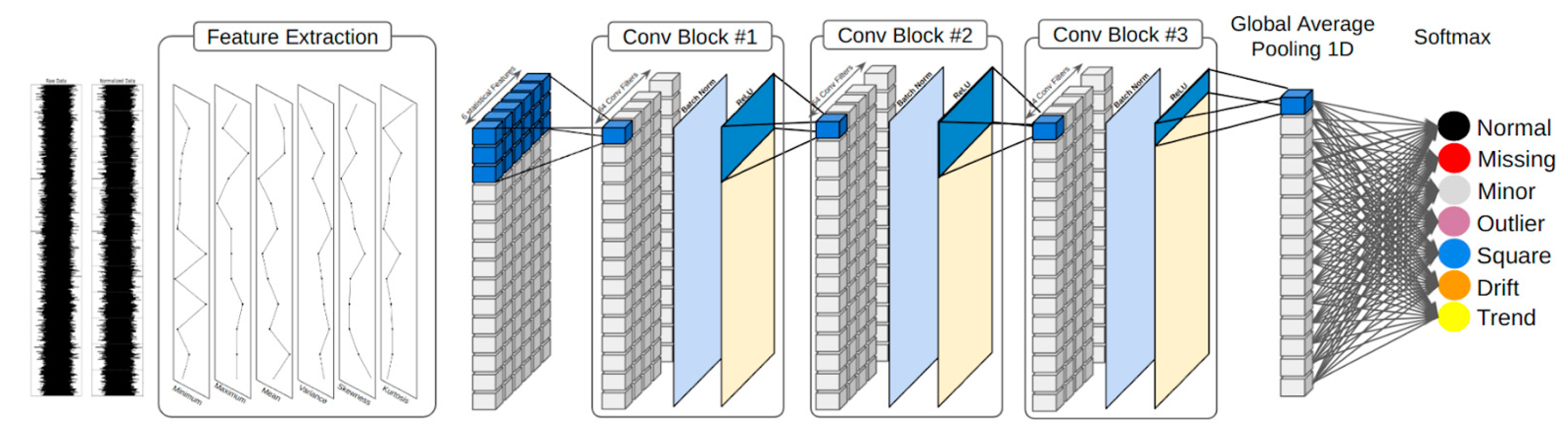
3.2. Feature Extraction
- Minimum (Min): This metric encapsulates the minimal observed value within a specific data segment. Its function is to capture the nadir of oscillations or vibrations during the stipulated interval, affording insights into the potential troughs of motion.
- Maximum (Max): Unlike the minimum, the maximum denotes the corresponding segment’s pinnacle value within the dataset. This metric illuminates data peaks, which might correspond to heightened stress or perturbation on the bridge structure.
- Mean: The mean, emblematic of the arithmetic average across a defined interval, furnishes a central reference point. It indicates the prevailing trend or behavioral pattern encompassing the dataset during the designated timeframe.
- Variance: As a pivotal gauge of dispersion, variance furnishes revelations into the degree of divergence exhibited by individual data points with the mean. Elevated variance values may allude to more capricious tendencies or pronounced fluctuations within the acceleration data.
- Skewness: This statistical measure scrutinizes the asymmetry or symmetry deficiency within the data distribution. Nonzero skewness values may allude to potential biases or consistent directional tendencies within the data, offering a glimpse into recurrent external influences or patterns impinging upon the bridge dynamics.
- Kurtosis: Offering a perspective into the tails of the data distribution, kurtosis appraises the extremeness of data points. Elevated kurtosis values signify a heightened prevalence of outliers or substantial peaks indicative of sporadic external perturbations or anomalous deviations within the bridge’s comportment.
3.3. D-CNN-Based Model Architecture
- Conv1D layer: Each convolutional block initiates with a 1D convolutional layer. We employ 64 filters, each characterized by a kernel size of 3. These filters function as discerners of patterns, gliding across the input sequence to discern localized patterns or configurations. Through the application of “same” padding, the output ensuing from this layer maintains a length equitably matched with the input, thereby preserving temporal information integrity. With a stride of 1, every filter meticulously scrutinizes all conceivable positions within the input sequence, engendering a comprehensive scan.
- Batch normalization layer: Subsequent to the convolutional operations, the dataset undergoes normalization within every minibatch. This normalization procedure stabilizes and hastens the learning trajectory. By nurturing a uniform data distribution within each batch, the training regimen acquires heightened resilience against potential fluctuations in feature values, culminating in swifter convergence and, frequently, enhanced generalization capabilities.
- ReLU activation function: Following normalization, a rectified linear unit (ReLU) activation function is enacted. This nonlinear function is entrusted with infusing nonlinearity into the model. The selection of ReLU derives from its computational efficiency and the ability to mitigate the challenge of vanishing gradients, thereby fostering more efficacious training for deep networks.
- Global average pooling 1D (GAP1D) layer: Following the sequence of convolutional blocks, the architecture of the model accommodates a GAP1D layer. In contrast to conventional pooling layers that curtail dimensionality by opting for maximum or average values within segments, the GAP1D layer averages the responses of all 64 filters across the entire temporal expanse. This begets an unchanging output dimensionality, succinctly capturing quintessential feature information while discarding extraneous or relatively less informative data.
- Softmax activation function: The conclusive layer within our architectural construct manifests as a fully connected layer endowed with softmax activation. Given the multiclass disposition of our problem—entailing the possibility of seven distinct classes—the softmax activation engenders the computation of the probability distribution across these classes. Each input is definitively aligned with the class characterized by the highest probability, thereby ensuring a lucid and categorical output.
4. Experimental Results
4.1. Data Collection and Preprocessing
4.2. Evaluation Metrics
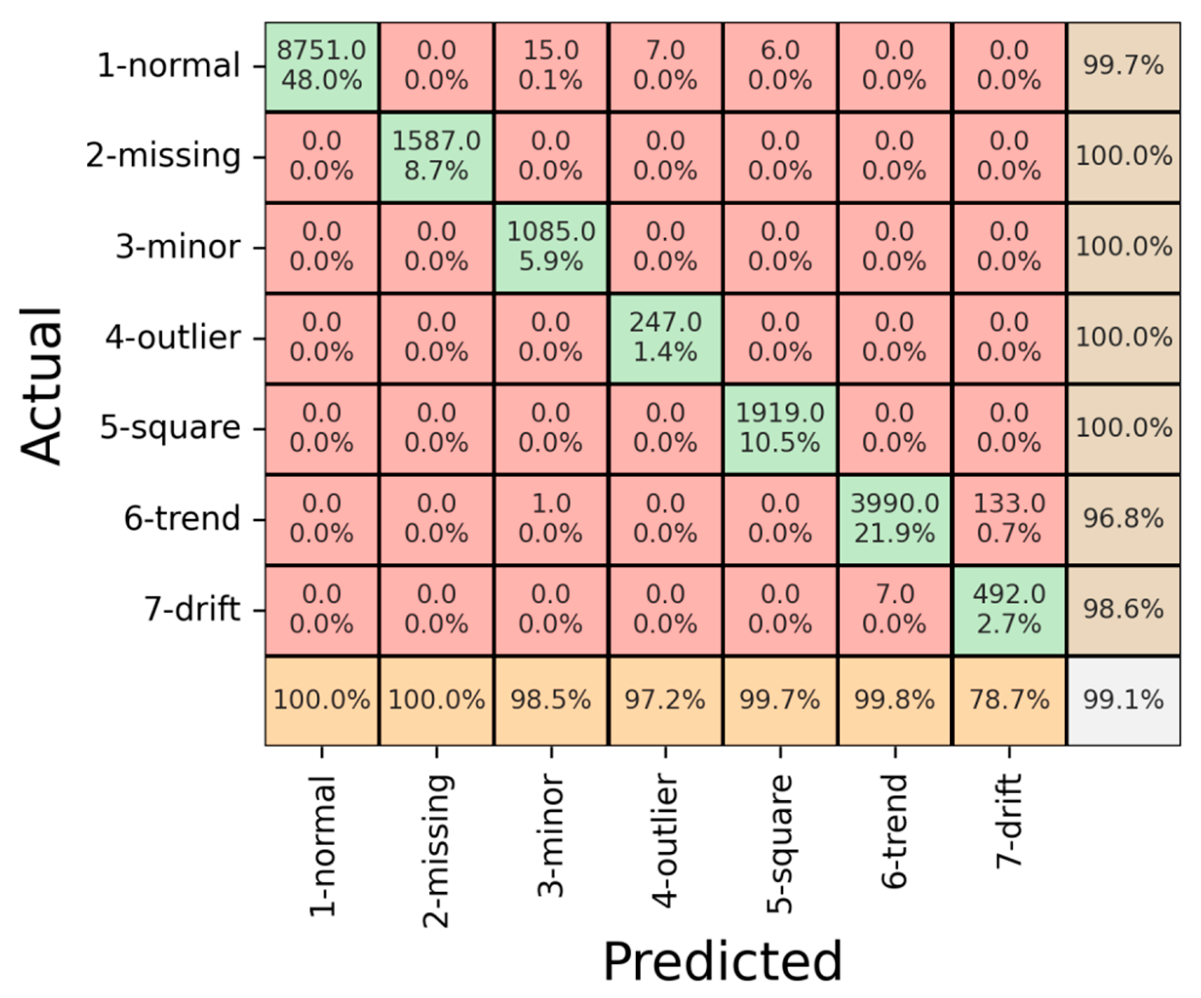
4.3. Results
5. Discussion
6. Conclusions
Author Contributions
Funding
Institutional Review Board Statement
Informed Consent Statement
Data Availability Statement
Acknowledgments
Conflicts of Interest
References
- Fu, Y.; Peng, C.; Gomez, F.; Narazaki, Y.; Spencer, B.F., Jr. Sensor fault management techniques for wireless smart sensor networks in structural health monitoring. Struct. Control Health Monit. 2019, 26, e2362. [Google Scholar] [CrossRef]
- Peng, C.; Fu, Y.; Spencer, B.F. Sensor fault detection, identification, and recovery techniques for wireless sensor networks: A full-scale study. In Proceedings of the 13th International Workshop on Advanced Smart Materials and Smart Structures Technology, Tokyo, Japan, 22–23 July 2017; pp. 22–23. [Google Scholar]
- Bao, Y.; Chen, Z.; Wei, S.; Xu, Y.; Tang, Z.; Li, H. The state of the art of data science and engineering in structural health monitoring. Engineering 2019, 5, 234–242. [Google Scholar] [CrossRef]
- Chang, C.M.; Chou, J.Y.; Tan, P.; Wang, L. A sensor fault detection strategy for structural health monitoring systems. Smart Struct. Syst. 2017, 20, 43–52. [Google Scholar]
- Lo, C.; Lynch, J.P.; Liu, M. Distributed model-based nonlinear sensor fault diagnosis in wireless sensor networks. Mech. Syst. Signal Process. 2016, 66, 470–484. [Google Scholar] [CrossRef]
- Peng, Y.; Qiao, W.; Qu, L.; Wang, J. Sensor fault detection and isolation for a wireless sensor network-based remote wind turbine condition monitoring system. IEEE Trans. Ind. Appl. 2017, 54, 1072–1079. [Google Scholar] [CrossRef]
- Huang, H.B.; Yi, T.H.; Li, H.N. Sensor fault diagnosis for structural health monitoring based on statistical hypothesis test and missing variable approach. J. Aerosp. Eng. 2017, 30, B4015003. [Google Scholar] [CrossRef]
- Li, L.; Liu, G.; Zhang, L.; Li, Q. Sensor fault detection with generalized likelihood ratio and correlation coefficient for bridge SHM. J. Sound Vib. 2019, 442, 445–458. [Google Scholar] [CrossRef]
- Huang, H.B.; Yi, T.H.; Li, H.N. Bayesian combination of weighted principal-component analysis for diagnosing sensor faults in structural monitoring systems. J. Eng. Mech. 2017, 143, 04017088. [Google Scholar] [CrossRef]
- Malekloo, A.; Ozer, E.; AlHamaydeh, M.; Girolami, M. Machine learning and structural health monitoring overview with emerging technology and high-dimensional data source highlights. Struct. Health Monit. 2022, 21, 1906–1955. [Google Scholar] [CrossRef]
- Mukhiddinov, M.; Muminov, A.; Cho, J. Improved Classification Approach for Fruits and Vegetables Freshness Based on Deep Learning. Sensors 2022, 22, 8192. [Google Scholar] [CrossRef]
- Avazov, K.; Abdusalomov, A.; Mukhiddinov, M.; Baratov, N.; Makhmudov, F.; Cho, Y.I. An improvement for the automatic classification method for ultrasound images used on CNN. Int. J. Wavelets Multiresolut. Inf. Process. 2022, 20, 2150054. [Google Scholar] [CrossRef]
- Ni, F.; Zhang, J.; Noori, M.N. Deep learning for data anomaly detection and data compression of a long-span suspension bridge. Comput.-Aided Civ. Infrastruct. Eng. 2020, 35, 685–700. [Google Scholar] [CrossRef]
- Zhang, Y.; Miyamori, Y.; Mikami, S.; Saito, T. Vibration-based structural state identification by a 1-dimensional convolutional neural network. Comput.-Aided Civ. Infrastruct. Eng. 2019, 34, 822–839. [Google Scholar] [CrossRef]
- Khamdamov, U.; Abdullayev, A.; Mukhiddinov, M.; Xalilov, S. Algorithms of multidimensional signals processing based on cubic basis splines for information systems and processes. J. Appl. Sci. Eng. 2021, 24, 141–150. [Google Scholar]
- Abdeljaber, O.; Avci, O.; Kiranyaz, S.; Gabbouj, M.; Inman, D.J. Real-time vibration-based structural damage detection using one-dimensional convolutional neural networks. J. Sound Vib. 2017, 388, 154–170. [Google Scholar] [CrossRef]
- Mukhiddinov, M.; Kim, S.-Y. A Systematic Literature Review on the Automatic Creation of Tactile Graphics for the Blind and Visually Impaired. Processes 2021, 9, 1726. [Google Scholar] [CrossRef]
- Obiechefu, C.B.; Kromanis, R.; Mohammad, F.; Arab, Z. Vision-Based Damage Detection Using Inclination Angles and Curvature. In International Workshop on Civil Structural Health Monitoring; Springer: Cham, Switzerland, 2021; pp. 115–127. [Google Scholar]
- Mukhiddinov, M.; Cho, J. Smart Glass System Using Deep Learning for the Blind and Visually Impaired. Electronics 2021, 10, 2756. [Google Scholar] [CrossRef]
- Cha, Y.J.; Choi, W.; Suh, G.; Mahmoudkhani, S.; Büyüköztürk, O. Autonomous structural visual inspection using region-based deep learning for detecting multiple damage types. Comput.-Aided Civ. Infrastruct. Eng. 2018, 33, 731–747. [Google Scholar] [CrossRef]
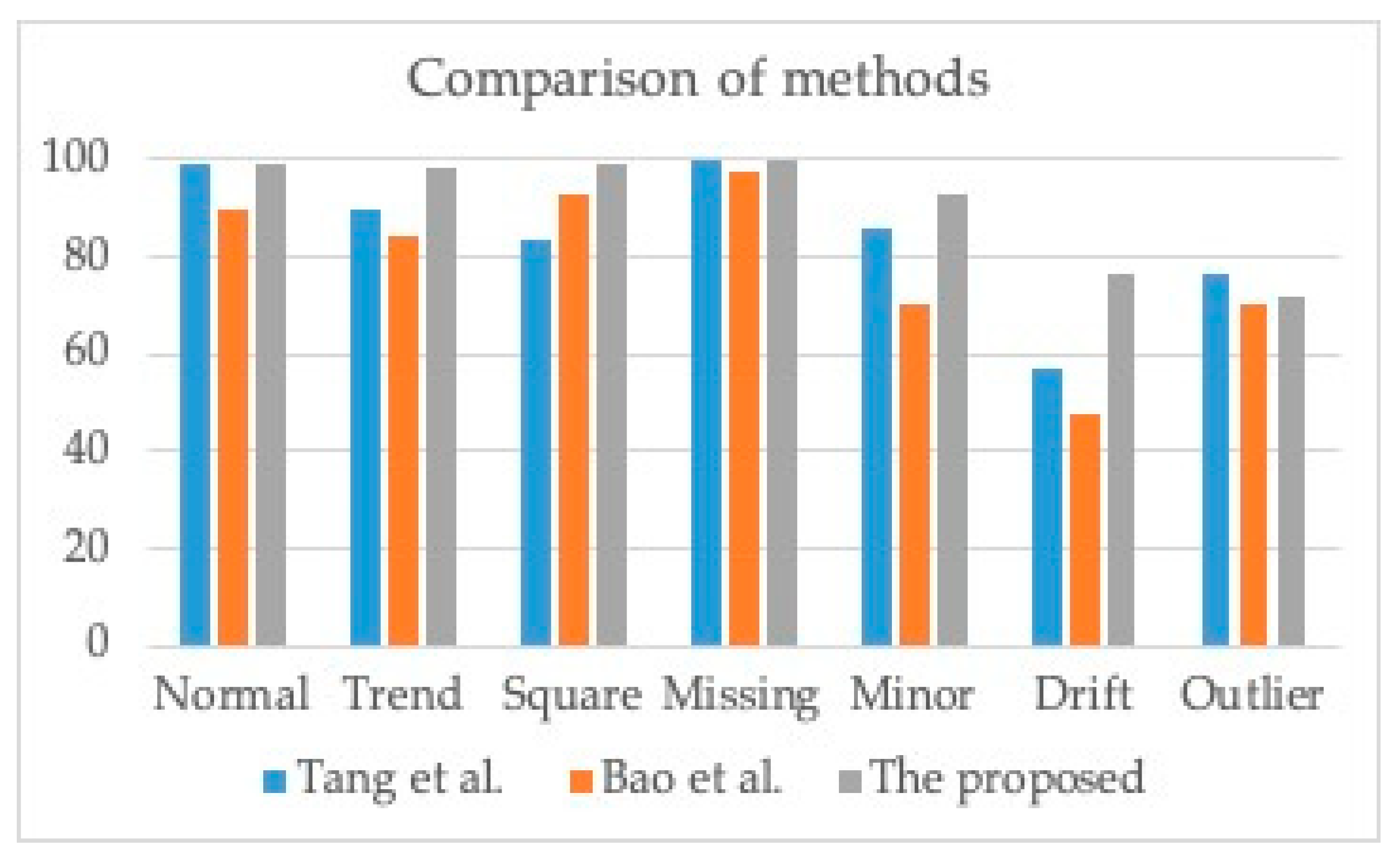
- Tang, Z.; Chen, Z.; Bao, Y.; Li, H. Convolutional neural network-based data anomaly detection method using multiple information for structural health monitoring. Struct. Control Health Monit. 2019, 26, e2296. [Google Scholar] [CrossRef]
- Makhmudov, F.; Mukhiddinov, M.; Abdusalomov, A.; Avazov, K.; Khamdamov, U.; Cho, Y.I. Improvement of the end-to-end scene text recognition method for “text-to-speech” conversion. Int. J. Wavelets Multiresolut. Inf. Process. 2020, 18, 2050052. [Google Scholar] [CrossRef]
- Farkhod, A.; Abdusalomov, A.B.; Mukhiddinov, M.; Cho, Y.-I. Development of Real-Time Landmark-Based Emotion Recognition CNN for Masked Faces. Sensors 2022, 22, 8704. [Google Scholar] [CrossRef]
- Mukhamadiyev, A.; Khujayarov, I.; Djuraev, O.; Cho, J. Automatic Speech Recognition Method Based on Deep Learning Approaches for Uzbek Language. Sensors 2022, 22, 3683. [Google Scholar] [CrossRef] [PubMed]
- Abdusalomov, A.B.; Mukhiddinov, M.; Kutlimuratov, A.; Whangbo, T.K. Improved Real-Time Fire Warning System Based on Advanced Technologies for Visually Impaired People. Sensors 2022, 22, 7305. [Google Scholar] [CrossRef] [PubMed]
- Avazov, K.; Mukhiddinov, M.; Makhmudov, F.; Cho, Y.I. Fire Detection Method in Smart City Environments Using a Deep-Learning-Based Approach. Electronics 2021, 1, 73. [Google Scholar] [CrossRef]
- Khamdamov, U.R.; Mukhiddinov, M.N.; Djuraev, O.N. An overview of deep learning based text spotting in natural scene images. Probl. Comput. Appl. Math. Tashkent 2019, 2, 126–134. [Google Scholar]
- Mukhiddinov, M. Scene Text Detection and Localization using Fully Convolutional Network. In Proceedings of the 2019 International Conference on Information Science and Communications Technologies (ICISCT), Tashkent, Uzbekistan, 4–6 November 2019; pp. 1–5. [Google Scholar]
- Entezami, A.; Sarmadi, H.; Behkamal, B. A novel double-hybrid learning method for modal frequency-based damage assessment of bridge structures under different environmental variation patterns. Mech. Syst. Signal Process. 2023, 201, 110676. [Google Scholar] [CrossRef]
- Entezami, A.; Sarmadi, H.; Behkamal, B.; De Michele, C. On continuous health monitoring of bridges under serious environmental variability by an innovative multi-task unsupervised learning method. Struct. Infrastruct. Eng. 2023, 1–19. [Google Scholar] [CrossRef]
- Pimentel, M.A.; Clifton, D.A.; Clifton, L.; Tarassenko, L. A review of novelty detection. Signal Process. 2014, 99, 215–249. [Google Scholar] [CrossRef]
- Li, H.; Wang, T.; Wu, G. A Bayesian deep learning approach for random vibration analysis of bridges subjected to vehicle dynamic interaction. Mech. Syst. Signal Process. 2022, 170, 108799. [Google Scholar] [CrossRef]
- Bao, Y.; Tang, Z.; Li, H.; Zhang, Y. Computer vision and deep learning–based data anomaly detection method for structural health monitoring. Struct. Health Monit. 2019, 8, 401–421. [Google Scholar] [CrossRef]
- Liu, G.; Niu, Y.; Zhao, W.; Duan, Y.; Shu, J. Data anomaly detection for structural health monitoring using a combination network of GANomaly and CNN. Smart Struct. Syst. 2022, 29, 53–62. [Google Scholar]
- Chou, J.Y.; Fu, Y.; Huang, S.K.; Chang, C.M. SHM data anomaly classification using machine learning strategies: A comparative study. Smart Struct. Syst. 2022, 29, 77–91. [Google Scholar]
- Mao, J.; Wang, H.; Spencer, B.F., Jr. Toward data anomaly detection for automated structural health monitoring: Exploiting generative adversarial nets and autoencoders. Struct. Health Monit. 2021, 20, 1609–1626. [Google Scholar] [CrossRef]
- Li, S.; Jin, X.; Xuan, Y.; Zhou, X.; Chen, W.; Wang, Y.X.; Yan, X. Enhancing the locality and breaking the memory bottleneck of transformer on time series forecasting. Adv. Neural Inf. Process. Syst. 2019, 32. [Google Scholar] [CrossRef]
- Lim, B.; Arık, S.Ö.; Loeff, N.; Pfister, T. Temporal fusion transformers for interpretable multi-horizon time series forecasting. Int. J. Forecast. 2021, 37, 1748–1764. [Google Scholar] [CrossRef]
- Ince, T.; Kiranyaz, S.; Eren, L.; Askar, M.; Gabbouj, M. Real-time motor fault detection by 1-D convolutional neural networks. IEEE Trans. Ind. Electron. 2016, 63, 7067–7075. [Google Scholar] [CrossRef]
- Kiranyaz, S.; Ince, T.; Gabbouj, M. Personalized monitoring and advance warning system for cardiac arrhythmias. Sci. Rep. 2017, 7, 9270. [Google Scholar] [CrossRef]
- Kiranyaz, S.; Ince, T.; Gabbouj, M. Real-time patient-specific ECG classification by 1-D convolutional neural networks. IEEE Trans. Biomed. Eng. 2015, 63, 664–675. [Google Scholar] [CrossRef]
- Scherer, D.; Müller, A.; Behnke, S. Evaluation of pooling operations in convolutional architectures for object recognition. In Proceedings of the International Conference on Artificial Neural Networks, Thessaloniki, Greece, 15–18 September 2010; Springer: Berlin/Heidelberg, Germany, 2010; pp. 92–101. [Google Scholar] [CrossRef]
- Zhang, X.; Chen, F.; Huang, R. A combination of RNN and CNN for attention-based relation classification. Procedia Comput. Sci. 2018, 131, 911–917. [Google Scholar] [CrossRef]
- Wu, H.; Gu, X. Towards dropout training for convolutional neural networks. Neural Netw. 2015, 71, 1–10. [Google Scholar] [CrossRef]
- Kuo, C.C.J. Understanding convolutional neural networks with a mathematical model. J. Vis. Commun. Image Represent. 2016, 41, 406–413. [Google Scholar] [CrossRef]
- Zhang, Y.; Liang, P.; Wainwright, M.J. Convexified convolutional neural networks. In Proceedings of the International Conference on Machine Learning, Sidney, Australia, 6–11 August 2017; pp. 4044–4053. [Google Scholar]
- Avci, O.O.; Abdeljaber, S.; Kiranyaz, D. Inman, Structural damage detection in real time: Implementation of 1D convolutional neural networks for SHM applications. In Structural Health Monitoring & Damage Detection, Proceedings of the Thirty-Fifth IMAC, a Conference and Exposition on Structural Dynamics; Niezrecki, C., Ed.; Springer International Publishing: Cham, Switzerland, 2017; Volume 7, pp. 49–54. [Google Scholar] [CrossRef]
- Dyke, S.J.; Bernal, D.; Beck, J.; Ventura, C. Experimental phase II of the structural health monitoring benchmark problem. In Proceedings of the 16th ASCE Engineering Mechanics Conference, Seattle, WA, USA, 16–18 July 2018. [Google Scholar]
- The 1st International Project Competition for Structural Health Monitoring. 2023. Available online: http://www.schm.org.cn/#/IPC-SHM,2020/project2 (accessed on 18 June 2023).


| Class Name | Description |
|---|---|
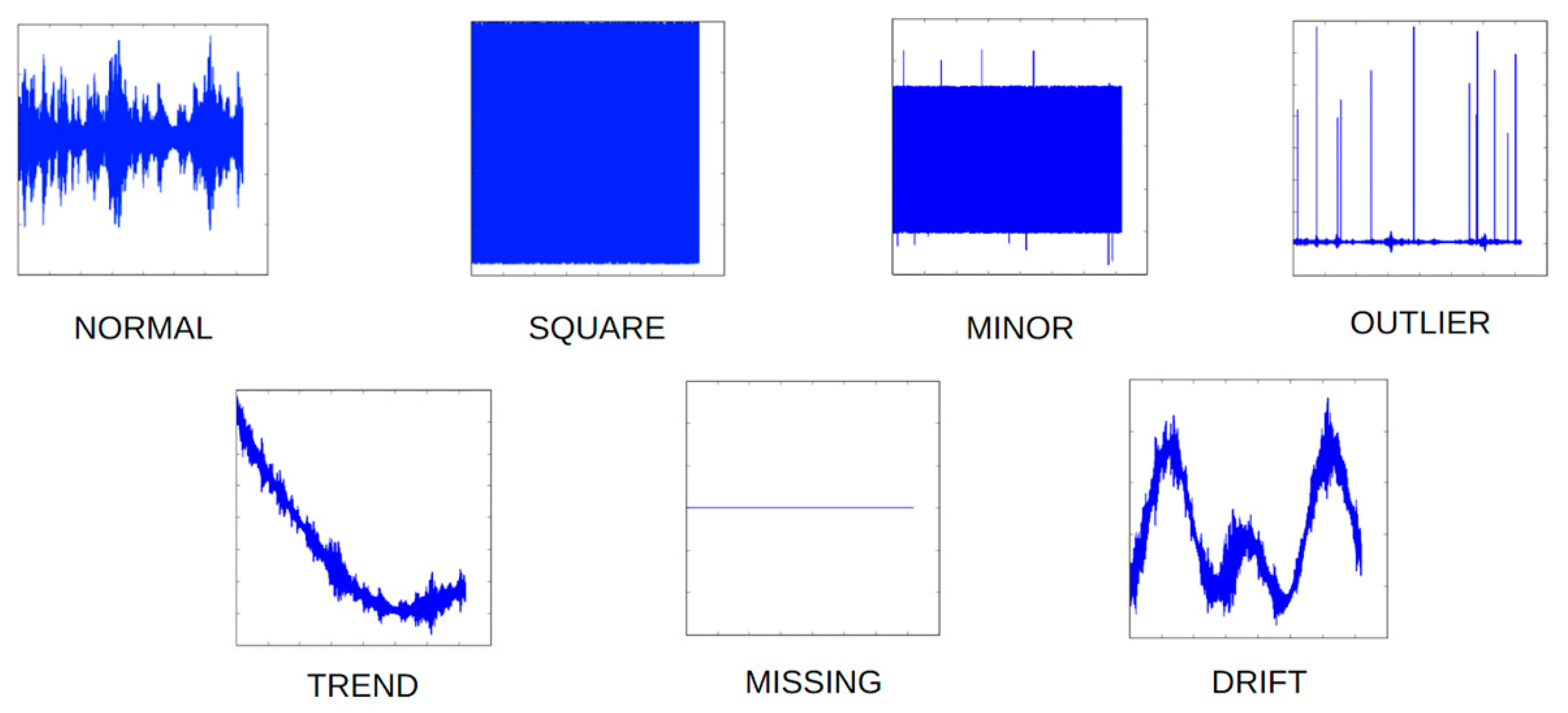
| Normal | The detectors reply in the time domain at a fluctuation angle with no noticeable marks. |
| Trend | The data have a noticeable gradient (up or down) in the time domain. |
| Square | The detector’s reply in the time domain is similar to a square wave. |
| Missing | The detector’s reply in the time domain is missing. |
| Minor | Compared to the typical sensor response considered normal, the amplitude within the time domain exhibits a minimal magnitude. |
| Drift | The response of the detector within the time domain is characterized by nonstationarity, leading to unforeseen drift phenomena. |
| Outlier | The detector’s reply lies outside the range typically observed for regular readings. |
| Class Name | Label | Before Data Augmentation | After Data Augmentation |
|---|---|---|---|
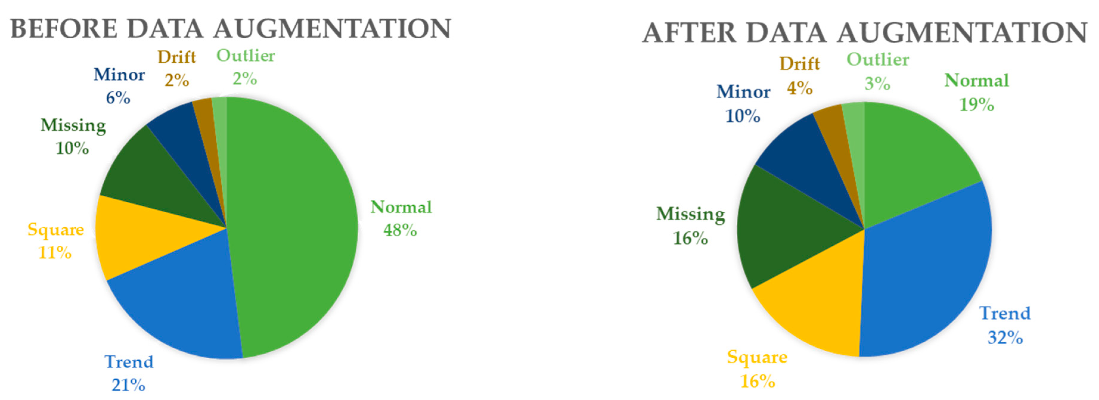
| Normal | 0 | 13,575 | 13,575 |
| Trend | 1 | 5778 | 23,112 |
| Square | 2 | 2996 | 11,984 |
| Missing | 3 | 2942 | 11,768 |
| Minor | 4 | 1775 | 7100 |
| Drift | 5 | 679 | 2716 |
| Outlier | 6 | 527 | 2108 |
| Total | 28,272 | 72,363 |
| Class Name | Training Data | Validation Data | Test Data | ||||||
|---|---|---|---|---|---|---|---|---|---|
| Precision | Recall | F1 Score | Precision | Recall | F1 Score | Precision | Recall | F1 Score | |
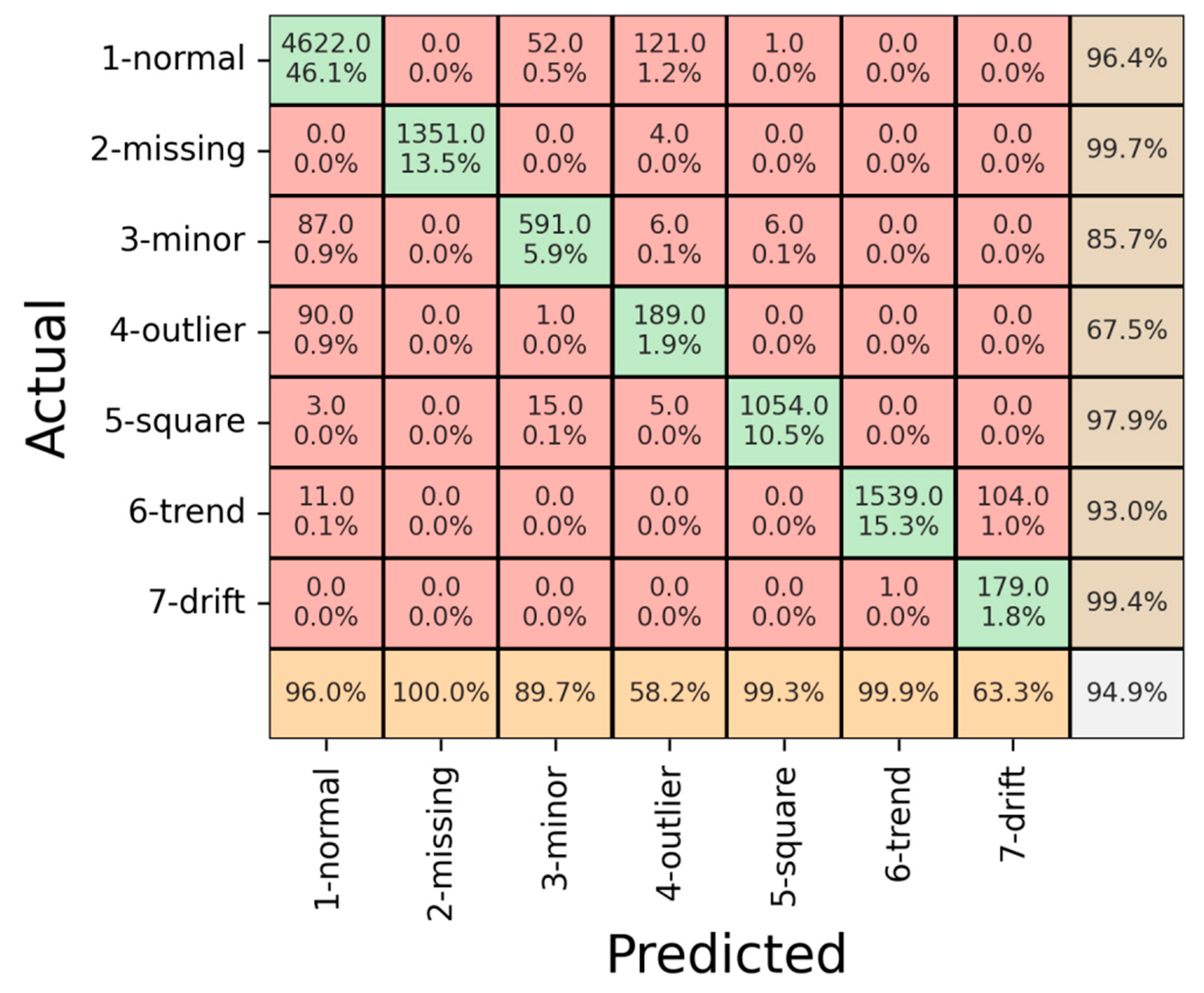
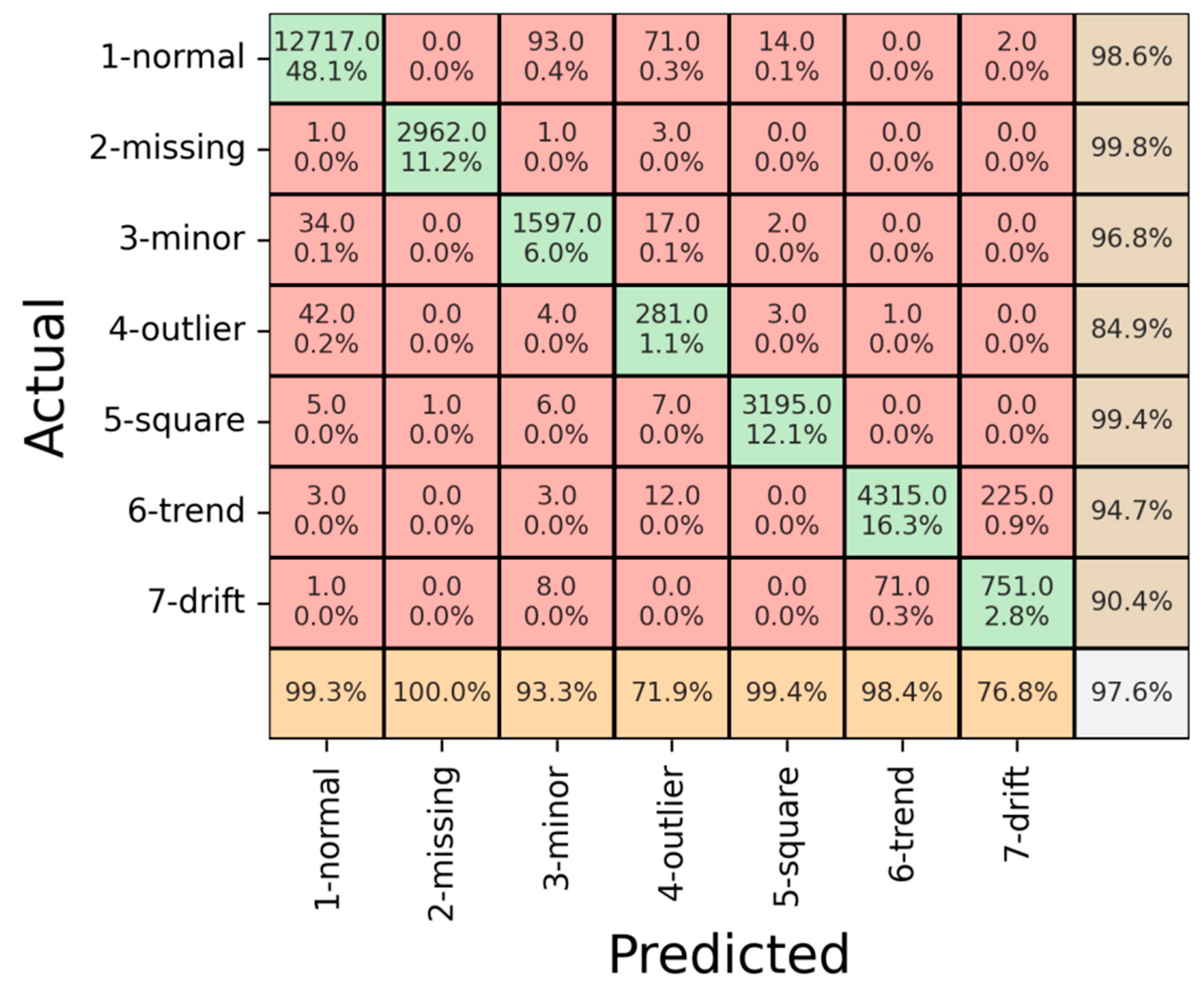
| Normal | 100% | 99.7% | 99.8% | 96% | 96.4% | 96.2% | 99.3% | 98.6% | 98.9% |
| Trend | 99.8% | 96.8% | 98.2% | 99.9% | 93% | 96.3% | 98.4% | 94.7% | 96.5% |
| Square | 99.7% | 100% | 99.8% | 99.3% | 97.9% | 98.5% | 99.4% | 99.4% | 99.4% |
| Missing | 100% | 100% | 100% | 100% | 99.7% | 99.8% | 100% | 99.8% | 99.9% |
| Minor | 98.5% | 100% | 99.2% | 89.7% | 85.7% | 87.6% | 93.3% | 96.8% | 95% |
| Drift | 78.7% | 98.6% | 87.5% | 63.3% | 99.4% | 77.3% | 76.8% | 90.4% | 83% |
| Outlier | 97.2% | 100% | 98.5% | 58.2% | 67.5% | 62.5% | 71.9% | 84.9% | 77.8% |
Disclaimer/Publisher’s Note: The statements, opinions and data contained in all publications are solely those of the individual author(s) and contributor(s) and not of MDPI and/or the editor(s). MDPI and/or the editor(s) disclaim responsibility for any injury to people or property resulting from any ideas, methods, instructions or products referred to in the content. |
© 2023 by the authors. Licensee MDPI, Basel, Switzerland. This article is an open access article distributed under the terms and conditions of the Creative Commons Attribution (CC BY) license (https://creativecommons.org/licenses/by/4.0/).
Share and Cite
Kim, S.-Y.; Mukhiddinov, M. Data Anomaly Detection for Structural Health Monitoring Based on a Convolutional Neural Network. Sensors 2023, 23, 8525. https://doi.org/10.3390/s23208525
Kim S-Y, Mukhiddinov M. Data Anomaly Detection for Structural Health Monitoring Based on a Convolutional Neural Network. Sensors. 2023; 23(20):8525. https://doi.org/10.3390/s23208525
Chicago/Turabian StyleKim, Soon-Young, and Mukhriddin Mukhiddinov. 2023. "Data Anomaly Detection for Structural Health Monitoring Based on a Convolutional Neural Network" Sensors 23, no. 20: 8525. https://doi.org/10.3390/s23208525
APA StyleKim, S.-Y., & Mukhiddinov, M. (2023). Data Anomaly Detection for Structural Health Monitoring Based on a Convolutional Neural Network. Sensors, 23(20), 8525. https://doi.org/10.3390/s23208525