
A Novel Tandem Differential Edge Sensor Layout for Segmented Mirror Telescopes


Abstract
:1. Introduction
2. Segmented Active Control Analysis
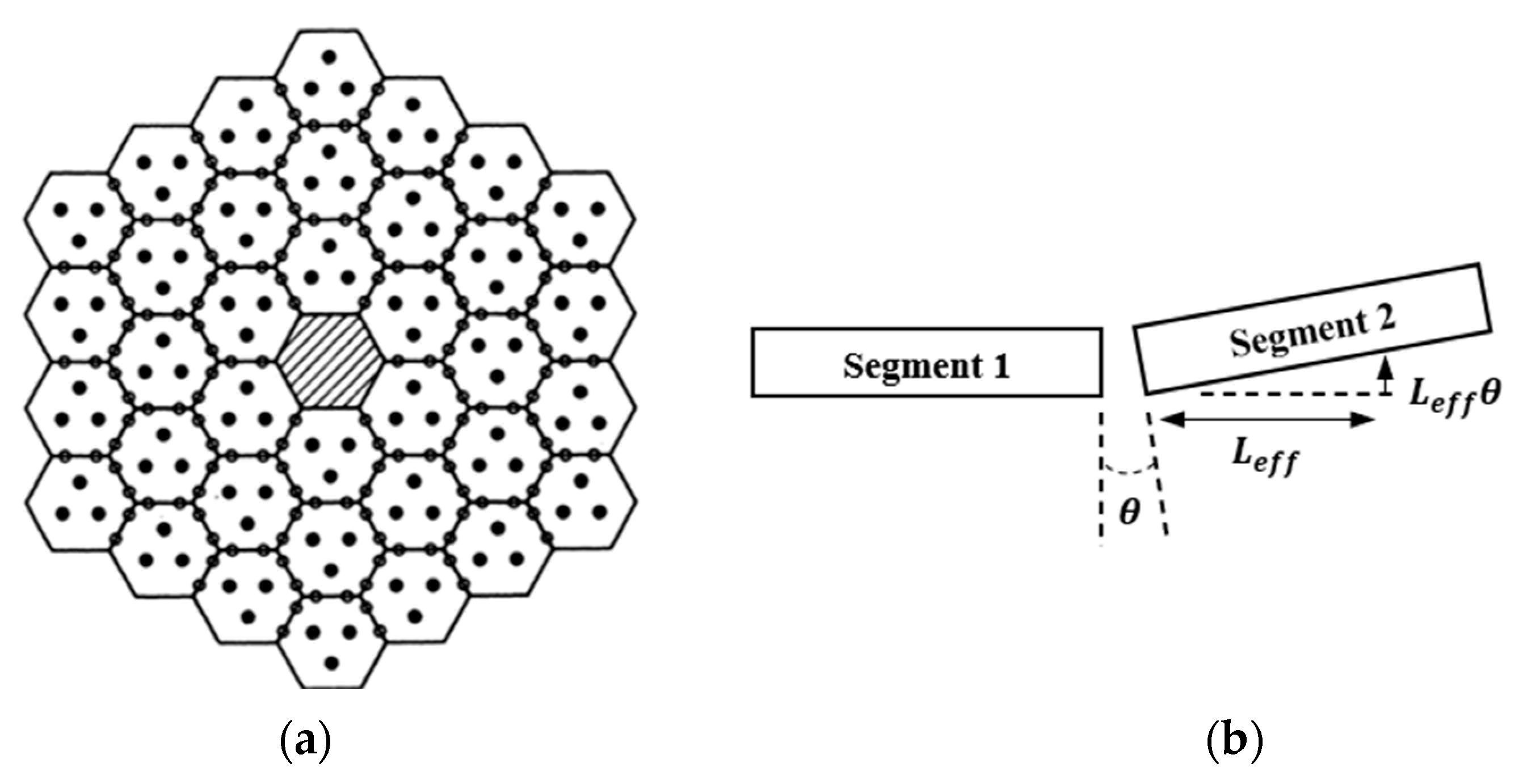
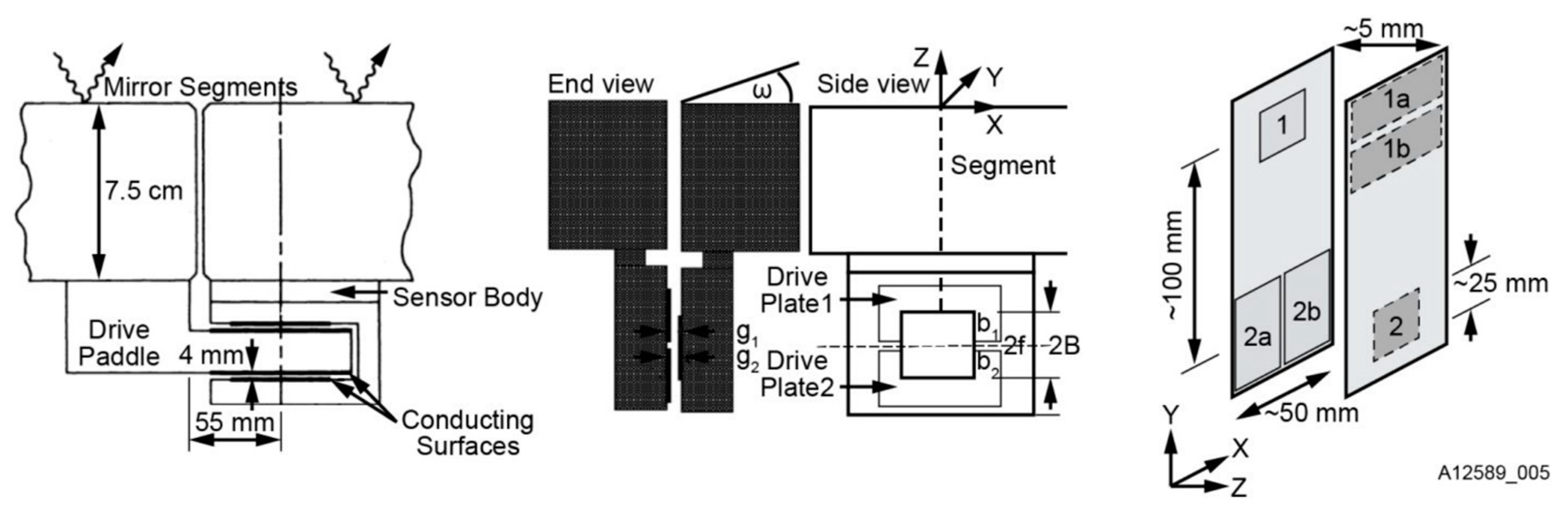
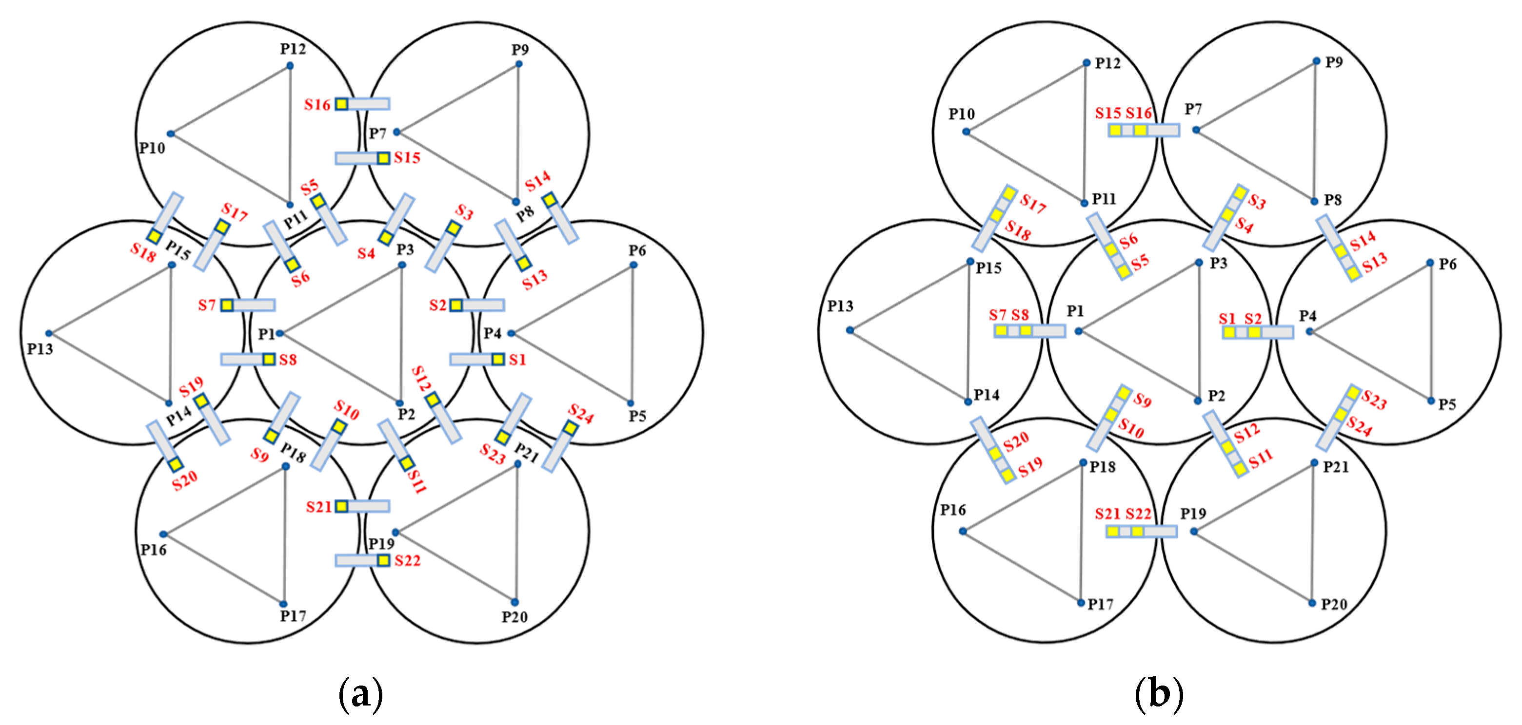
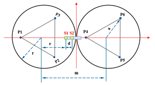
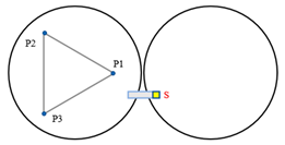
2.1. The Layout of the Edge Sensor Structure
2.2. Segmented Mirror Active Control
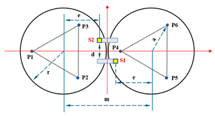
- where to represent the response coefficients of the sensors and actuators, which were determined using the methods described in the Appendix A. to represent the variations in readings of adjacent sensors from their ideal values, and to represent the displacements corresponding to the actuators P1 to P6. The position of the segmented mirror is determined by the arithmetic superposition of the independent movements of three actuators. Therefore, we have the following equation:
2.3. Singular Value Decomposition (SVD)
3. Control Performance of the Sensor Layout Scheme
3.1. Determination of Sensor Layout Parameters
- 1.
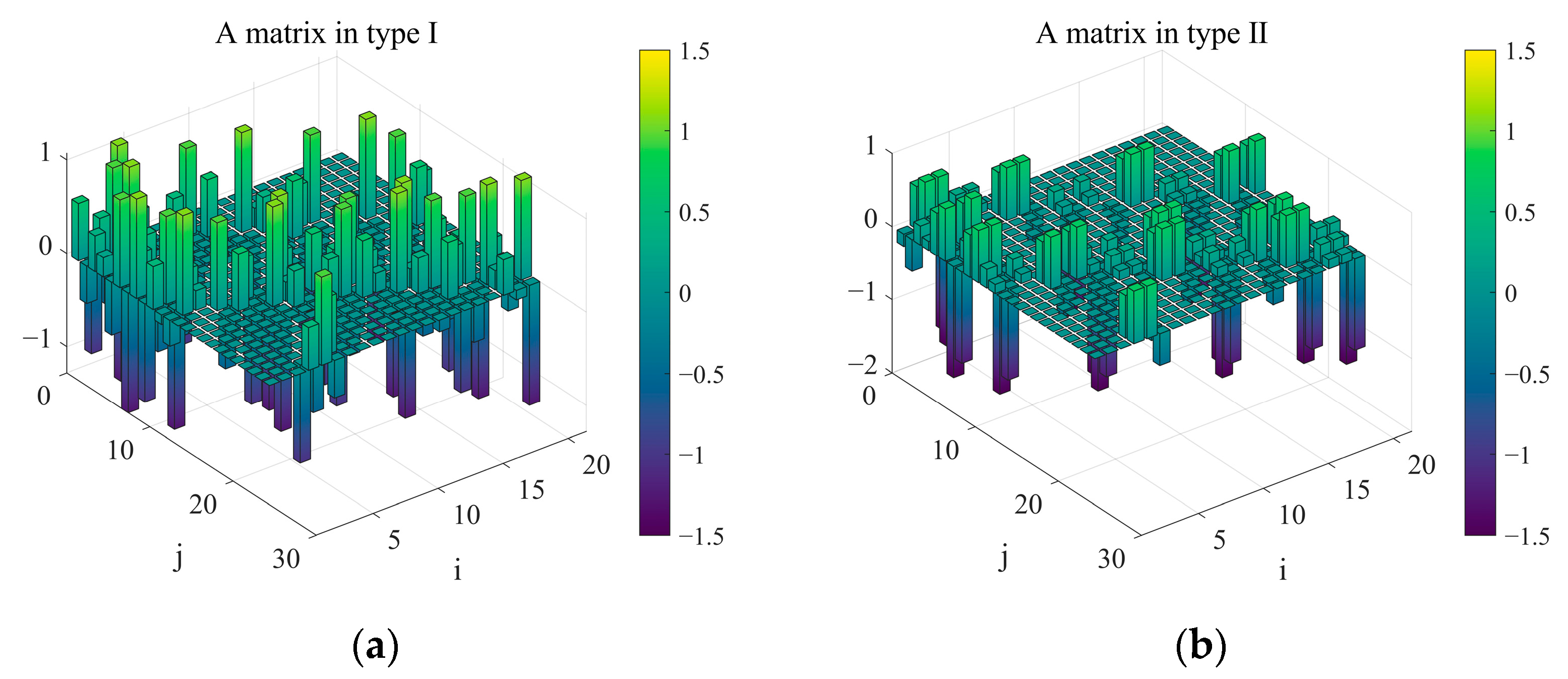
- In type I, the minimum non-zero singular value is primarily negatively correlated with and has low sensitivity to variations in . An increase in e represents an increase in the sensor’s measuring arm. However, when increases to m, the sensor’s sensitivity to the dihedral angle between adjacent sub-mirrors decreases to 0. This results in an undetectable fourth mode (focus mode), consistent with Keck’s analysis;
- 2.
- In type II, the minimum non-zero singular value is primarily positively correlated with and is almost insensitive to variations in . An increase in represents an increase in the sensor’s measuring arm;
- 3.
- For the same primary mirror configuration, the maximum value of the smallest non-zero singular value for type I is approximately twice that of type II.
3.2. Comparison of Control Performance between the Two Sensor Layout Types
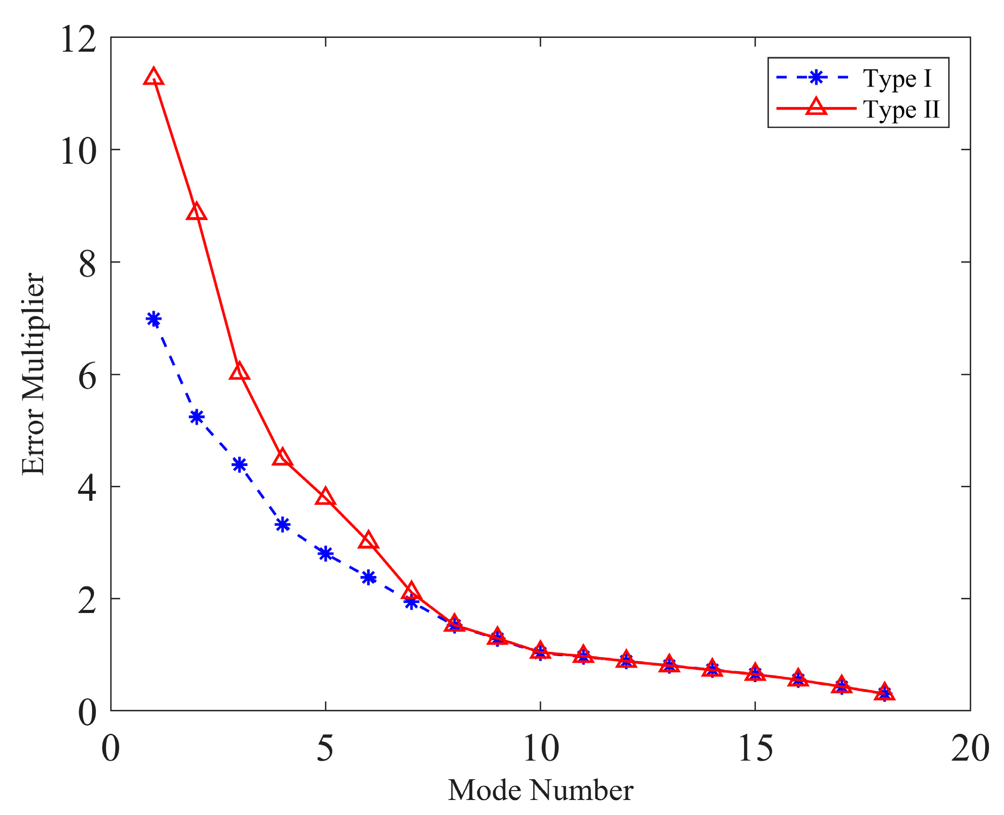
3.2.1. Error Propagation of the Control System
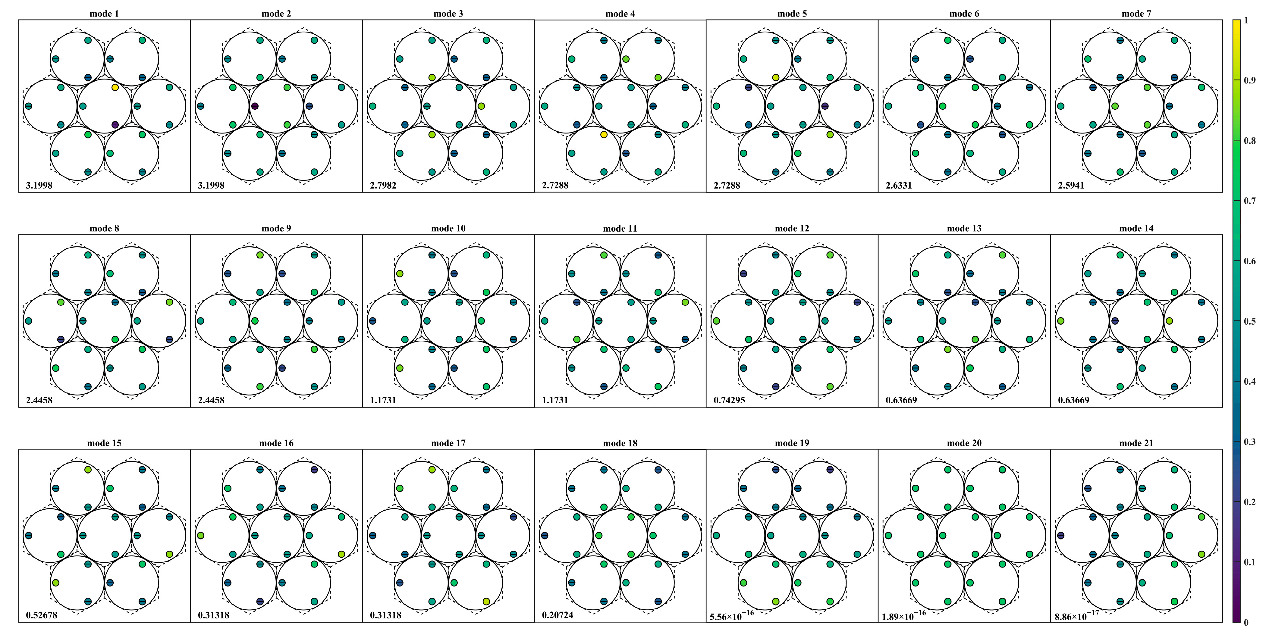
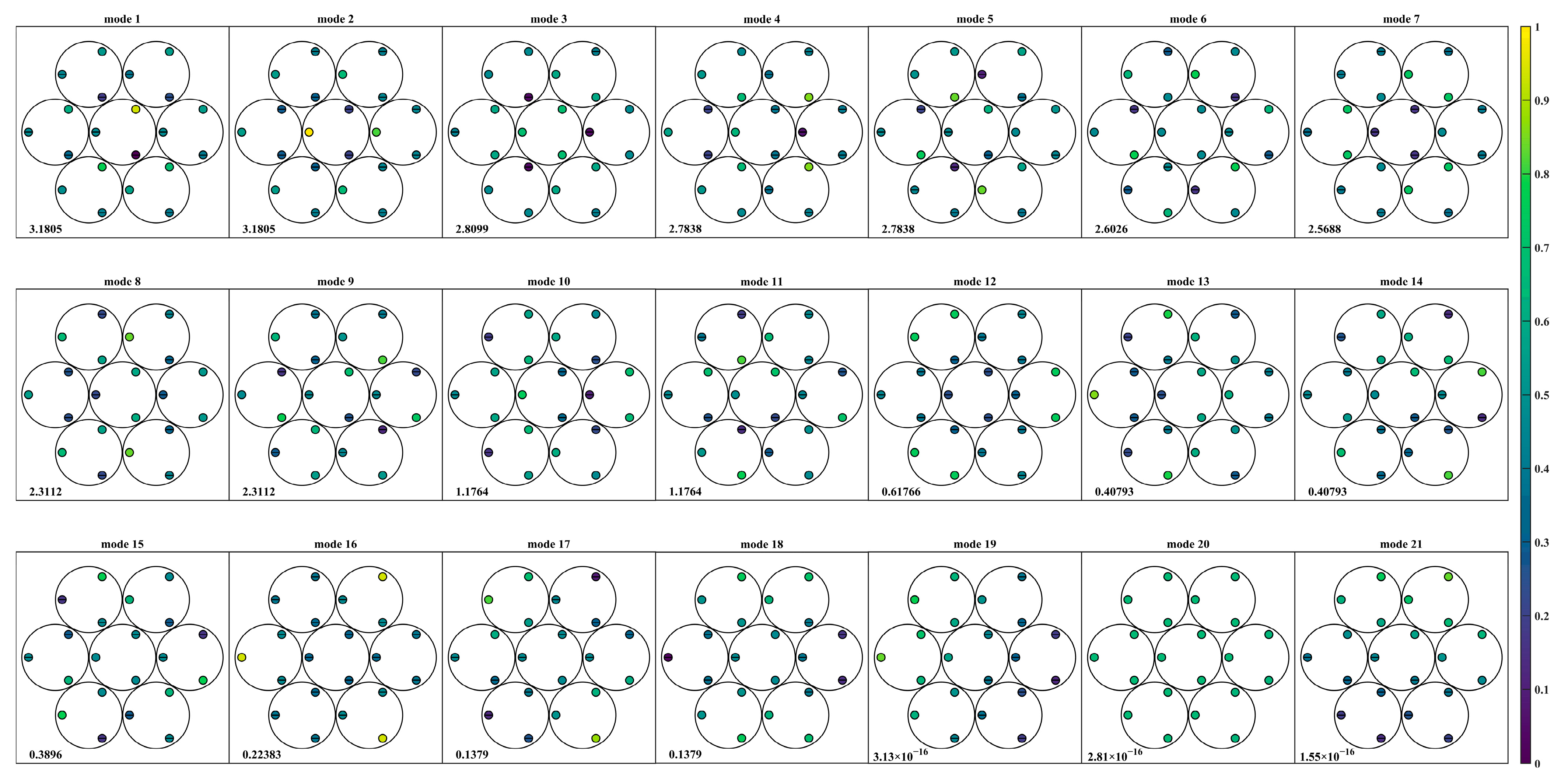
3.2.2. Characterization of the Actuator Modification Mode
3.2.3. Scalability Analysis of the Control Matrix
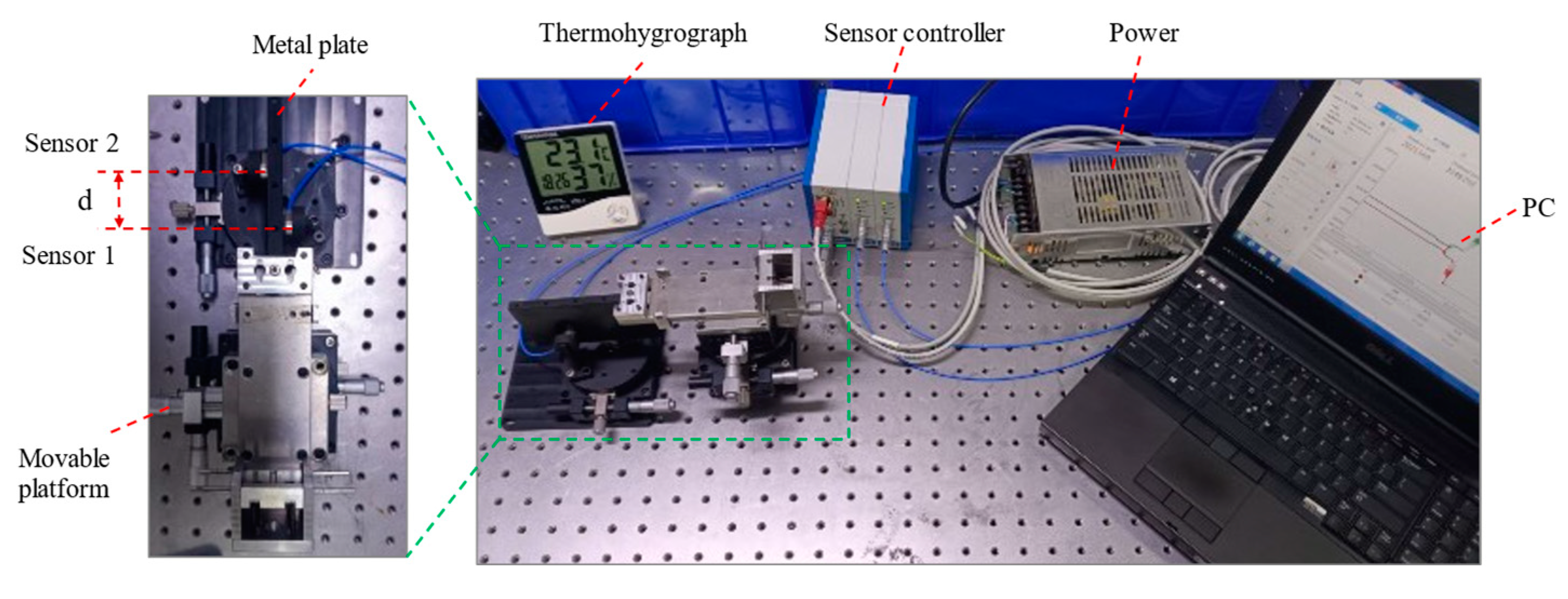
4. Experiment
5. Summary and Conclusions
Author Contributions
Funding
Institutional Review Board Statement
Informed Consent Statement
Data Availability Statement
Acknowledgments
Conflicts of Interest
Appendix A
References
- Kim, D.; Choi, H.; Brendel, T.; Quach, H.; Esparza, M.; Kang, H.; Feng, Y.-T.; Ashcraft, J.N.; Ke, X.; Wang, T.; et al. Advances in optical engineering for future telescopes. Opto-Electron. Adv. 2021, 4, 210040. [Google Scholar] [CrossRef]
- National Academies of Sciences, Engineering, and Medicine. Pathways to Discovery in Astronomy and Astrophysics for the 2020s; The National Academies Press: Washington, DC, USA, 2021; p. 615. [Google Scholar]
- Yin-long, H.; Fei, Y.; Fu-guo, W. Overview of key technologies for segmented mirrors of large-aperture optical telescopes. Chin. Opt. 2022, 15, 973–982. [Google Scholar] [CrossRef]
- Zhang, B.; Yang, F.; Wang, F.; Lu, B. Active Optics and Aberration Correction Technology for Sparse Aperture Segmented Mirrors. Appl. Sci. 2023, 13, 4063. [Google Scholar] [CrossRef]
- Wang, B.; Dai, Y.; Jin, Z.; Yang, D.; Xu, F. Active maintenance of a segmented mirror based on edge and tip sensing. Appl. Opt. 2021, 60, 7421–7431. [Google Scholar] [CrossRef] [PubMed]
- Stepp, L.M.; MacDonald, D.; Gilmozzi, R.; Woody, D.; Bradford, C.M.; Chamberlin, R.; Dragovan, M.; Goldsmith, P.; Radford, S.; Sebring, T.; et al. Cornell Caltech Atacama Telescope primary mirror surface sensing and controllability. In Ground-based and Airborne Telescopes II, Proceedings of the SPIE Astronomical Telescopes + Instrumentation, Marseille, France, 23–28 June 2008; SPIE: Bellingham, WA, USA, 2008. [Google Scholar]
- Lu, X.; Tian, G.; Wang, Z.; Li, W.; Yang, D.; Li, H.; Wang, Y.; Ni, J.; Zhang, Y. Research on the Time Drift Stability of Differential Inductive Displacement Sensors with Frequency Output. Sensors 2022, 22, 6234. [Google Scholar] [CrossRef] [PubMed]
- Barr, L.D.; Mast, T.S.; Gabor, G.; Nelson, J.E.; Mack, B. Edge Sensors for A Segmented Mirror. In Advanced Technology Optical Telescopes II, Proceedings of the 1983 Astronomy Conferences, London, UK, 5–9 September 1983; SPIE: Bellingham, WA, USA, 1983; pp. 297–309. [Google Scholar]
- Macmynowski, D.G. Interaction matrix uncertainty in active (and adaptive) optics. Appl. Opt. 2009, 48, 2105–2114. [Google Scholar] [CrossRef] [PubMed]
- Stepp, L.M.; Shelton, C.; Gilmozzi, R.; Mast, T.; Chanan, G.; Nelson, J.; Roberts, J.L.C.; Troy, M.; Sirota, M.J.; Seo, B.-J.; et al. Advances in edge sensors for the Thirty Meter Telescope primary mirror. In Ground-Based and Airborne Telescopes II, Proceedings of the SPIE Astronomical Telescopes + Instrumentation, Marseille, France, 23–28 June 2008; SPIE: Bellingham, WA, USA, 2008. [Google Scholar]
- Coyle, L.; Knight, J.S.; Adkins, M. Edge sensor concept for segment stabilization. In Space Telescopes and Instrumentation 2018: Optical, Infrared, and Millimeter Wave, Proceedings of the SPIE Astronomical Telescopes + Instrumentation, Austin, TX, USA, 10–15 June 2018; SPIE: Bellingham, WA, USA, 2018; Volume 10698. [Google Scholar]
- Burge, J.H.; Kendrick, S.E.; Fähnle, O.W.; Williamson, R. Monolithic versus segmented primary mirror concepts for space telescopes. In Optical Manufacturing and Testing VIII, Proceedings of the SPIE Optical Engineering + Applications, San Diego, CA, USA, 2–6 August 2009; SPIE: Bellingham, WA, USA, 2009. [Google Scholar]
- Haifeng, C. Research on the Technologies of Active Optics for Large aperture Segmented Optical/Infrared Telescope. Doctoral Thesis, University of Chinese Academy of Sciences (Changchun Institute of Optics, Fine Mechanics and Physics), Changchun, China, 2020. [Google Scholar]
- Barr, L.D.; Jared, R.C.; Arthur, A.A.; Andreae, S.; Biocca, A.K.; Cohen, R.W.; Fuertes, J.M.; Franck, J.; Gabor, G.; Llacer, J.; et al. Keck Telescope segmented primary mirror active control system. In Advanced Technology Optical Telescopes IV, Proceedings of the SPIE Astronomical Telescopes and Instrumentation for the 21st Century, Tucson, AZ, USA, 11–16 February 1990; SPIE: Bellingham, WA, USA, 1990; pp. 996–1008. [Google Scholar]
- Yin, J.; Zhao, G.; Feng, Z.; Ni, J. A Novel Dual-Differential Edge Sensor Based on the Eddy Current Effect. IEEE Sens. J. 2023, 23, 6129–6138. [Google Scholar] [CrossRef]
- Angel, J.R.P.; Angeli, G.Z.; Gilmozzi, R.; Cho, M.K.; Whorton, M.S. Active optics and control architecture for a giant segmented mirror telescope. In Future Giant Telescopes, Proceedings of the Astronomical Telescopes and Instrumentation, Waikoloa, HI, USA, 22–28 August 2002; SPIE: Bellingham, WA, USA, 2003. [Google Scholar]
- Zou, W. Generalized figure-control algorithm for large segmented telescope mirrors. J. Opt. Soc. Am. A 2001, 18, 638–649. [Google Scholar] [CrossRef]
- Hai-feng, C.; Jing-xu, Z.; Fei, Y.; Qi-chang, A. Application of ridge regression in pose control of telescope primary mirror with sparse aperture. Infrared Laser Eng. 2019, 48, 318003. [Google Scholar] [CrossRef]
- Deshmukh, P.; Mishra, D.S.; Parihar, P.; Vedashree. Primary mirror active control system simulation of Prototype Segmented Mirror Telescope. In Proceedings of the 2017 Indian Control Conference (ICC), Guwahati, India, 4–6 January 2017; pp. 364–371. [Google Scholar]
- Stepp, L.M.; Shimono, A.; Iwamuro, F.; Kurita, M.; Moritani, Y.; Kino, M.; Maihara, T.; Izumiura, H.; Yoshida, M.; Gilmozzi, R.; et al. Control algorithm for the petal-shape segmented-mirror telescope with 18 mirrors. In Ground-based and Airborne Telescopes IV, Proceedings of the SPIE Astronomical Telescopes + Instrumentation, Amsterdam, The Netherlands, 1–6 July 2012; SPIE: Bellingham, WA, USA, 2012. [Google Scholar]
- Nelson, J.; Mast, T.; Chanan, G. Segmented Mirror Telescopes. In Planets, Stars and Stellar Systems; Springer: Berlin/Heidelberg, Germany, 2013; pp. 99–136. [Google Scholar]
- Chanan, G.; MacMartin, D.G.; Nelson, J.; Mast, T. Control and alignment of segmented-mirror telescopes: Matrices, modes, and error propagation. Appl. Opt. 2004, 43, 1223–1232. [Google Scholar] [CrossRef] [PubMed]
- Miao, H.; Qi, Y. Pre-research on arithmetic for facing control of segmented-mirror in LAMOST. In Advanced Software and Control for Astronomy II, Proceedings of the SPIE Astronomical Telescopes + Instrumentation, Marseille, France, 23–28 June 2008; SPIE: Bellingham, WA, USA, 2008. [Google Scholar]
- Szeto, K.; Roberts, S.C.; Gedig, M.H.; Austin, G.; Lagally, C.D.; Patrick, S.; Tsang, D.; MacMynowski, D.G.; Sirota, M.J.; Stepp, L.M.; et al. TMT telescope structure system: Design and development progress report. In Ground-Based and Airborne Telescopes II, Proceedings of the Astronomical Telescopes + Instrumentation, Proceedings of the SPIE Astronomical Telescopes + Instrumentation, Marseille, France, 23–28 June 2008; SPIE: Bellingham, WA, USA, 2008. [Google Scholar]


| Keck | TMT | E-ELT | LAMOST | SALT | Seimei | |
|---|---|---|---|---|---|---|
| Type | Capacitive | Capacitive | Eddy current | Eddy current | Inductive | Inductive |
| Quantity | 168 | 2952 | 4924 | 290 | 546 | 72 |
| Range | ±12 μm | ±500 μm | ±200 μm | ±1 μm | 100 μm | — |
| Resolution (rms) | <2.5 nm | <5 nm | <5 nm | <1 nm | 1 nm | <2 nm |
| Temperature drift (rms) | 3 nm/°C | 1 nm/°C | 10 nm/°C | 6 nm/°C | 3.5 nm/°C | — |
| Time drift | 6 nm/week | 3 nm/week | 10 nm/week | — | 10 nm/week | 30 nm/night |
| Layout type | horizontal | vertical | vertical | horizontal | Vertical | horizontal |
| 55 mm | 32 mm | ≥10 mm | — | — | 50 mm |
| Type I | Type II 1 |
|---|---|
 |  |
| Type I | 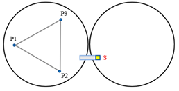 |  |
 |  | |
| Type II |  | 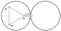 |
 |  |
Disclaimer/Publisher’s Note: The statements, opinions and data contained in all publications are solely those of the individual author(s) and contributor(s) and not of MDPI and/or the editor(s). MDPI and/or the editor(s) disclaim responsibility for any injury to people or property resulting from any ideas, methods, instructions or products referred to in the content. |
© 2023 by the authors. Licensee MDPI, Basel, Switzerland. This article is an open access article distributed under the terms and conditions of the Creative Commons Attribution (CC BY) license (https://creativecommons.org/licenses/by/4.0/).
Share and Cite
Huo, Y.; Yang, F.; Wang, F.; Guo, P.; Zhu, J.; Liu, Y. A Novel Tandem Differential Edge Sensor Layout for Segmented Mirror Telescopes. Sensors 2023, 23, 7252. https://doi.org/10.3390/s23167252
Huo Y, Yang F, Wang F, Guo P, Zhu J, Liu Y. A Novel Tandem Differential Edge Sensor Layout for Segmented Mirror Telescopes. Sensors. 2023; 23(16):7252. https://doi.org/10.3390/s23167252
Chicago/Turabian StyleHuo, Yinlong, Fei Yang, Fuguo Wang, Peng Guo, Jiakang Zhu, and Yuanguo Liu. 2023. "A Novel Tandem Differential Edge Sensor Layout for Segmented Mirror Telescopes" Sensors 23, no. 16: 7252. https://doi.org/10.3390/s23167252
APA StyleHuo, Y., Yang, F., Wang, F., Guo, P., Zhu, J., & Liu, Y. (2023). A Novel Tandem Differential Edge Sensor Layout for Segmented Mirror Telescopes. Sensors, 23(16), 7252. https://doi.org/10.3390/s23167252