

Improving APT Systems’ Performance in Air via Impedance Matching and 3D-Printed Clamp


Abstract
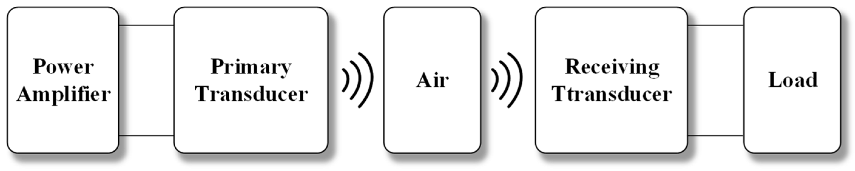
1. Introduction
2. Matching Theory of Acoustic Impedance
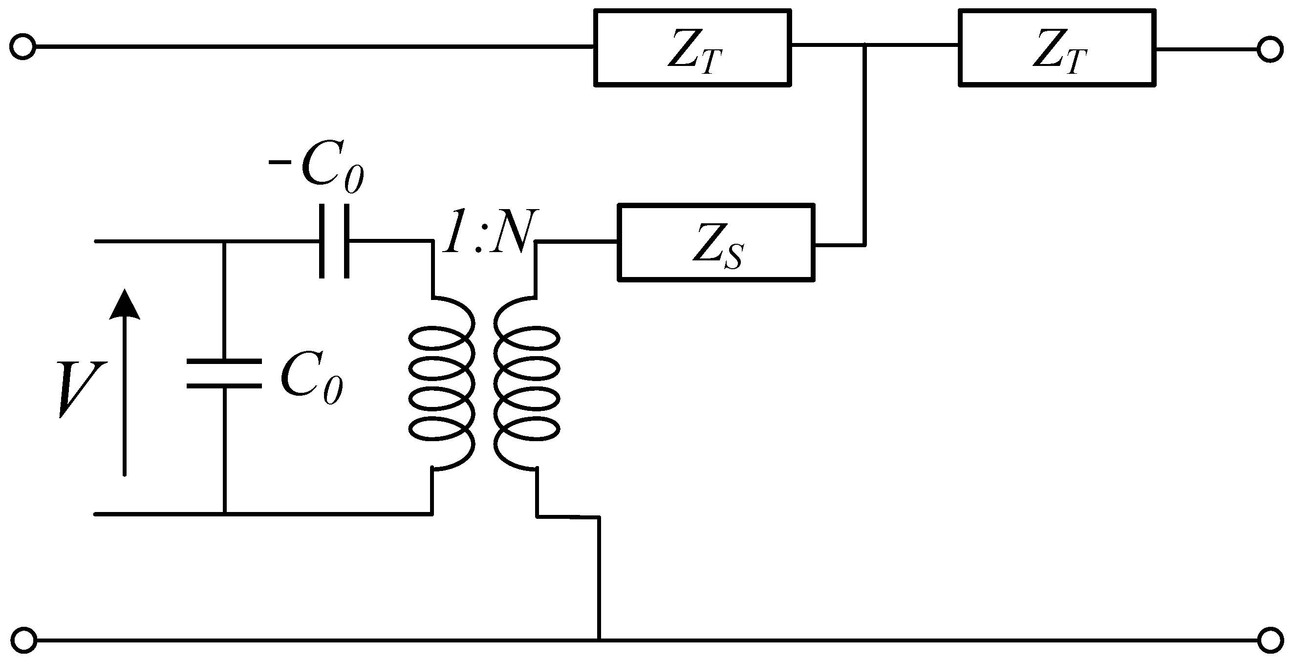
2.1. Impedance Matching Equivalent Circuit
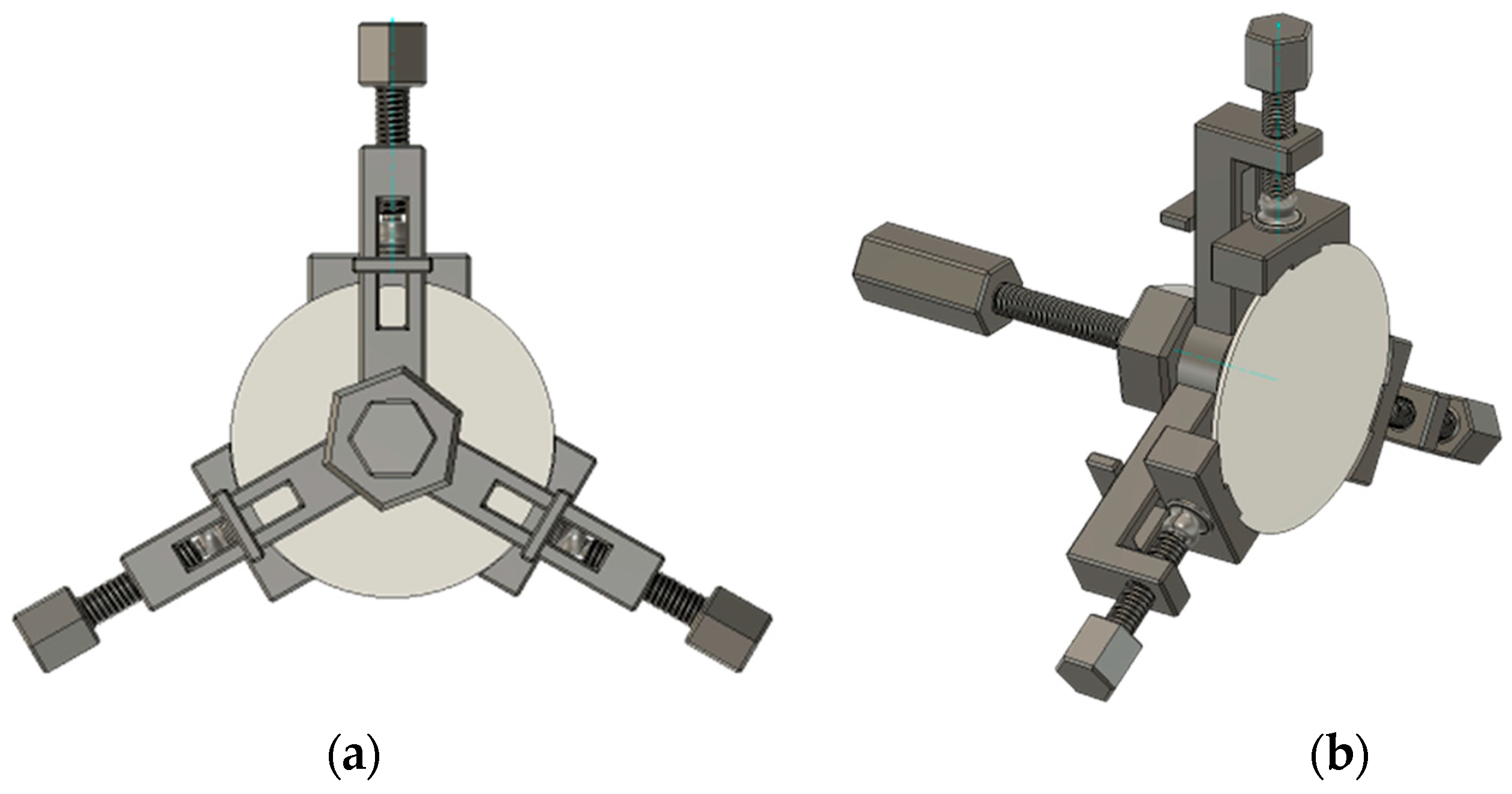
2.2. Proposed Approach for Impedance Matching—The Clamp of Piezoelectric Transducer
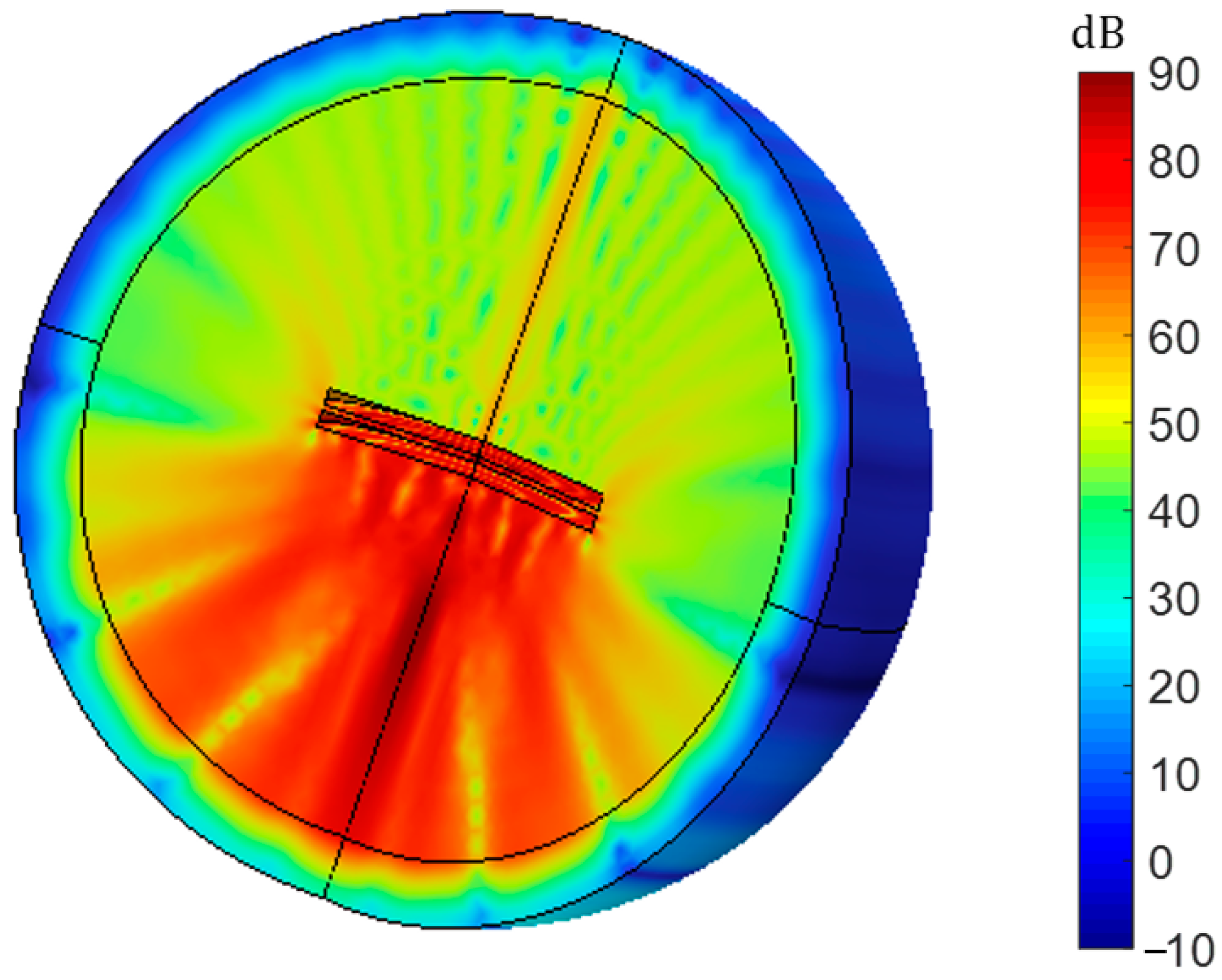
3. Simulation and Experimental Verification
3.1. The Clamp of Piezoelectric Transducers
3.1.1. No Clamp
3.1.2. Back Clamp
3.1.3. Peripheral Clamp
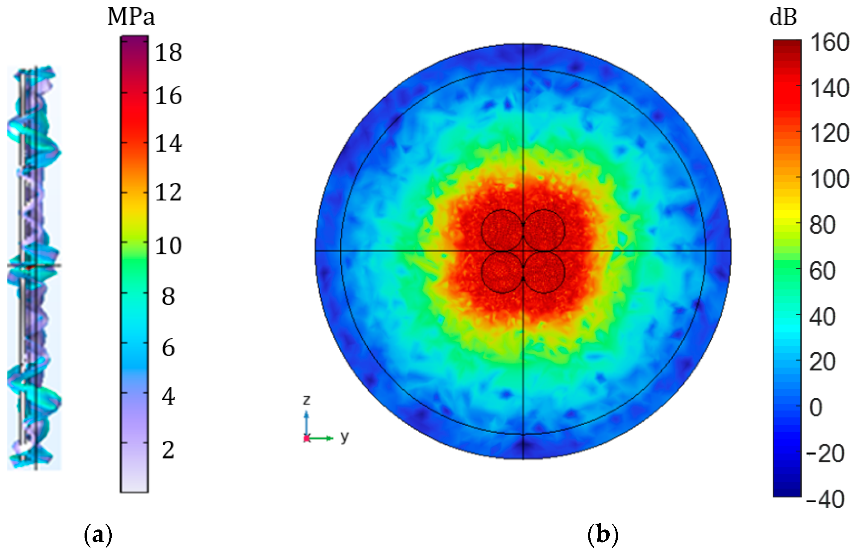
3.1.4. Piezoelectric Transducer Array
3.2. Experimental Verification
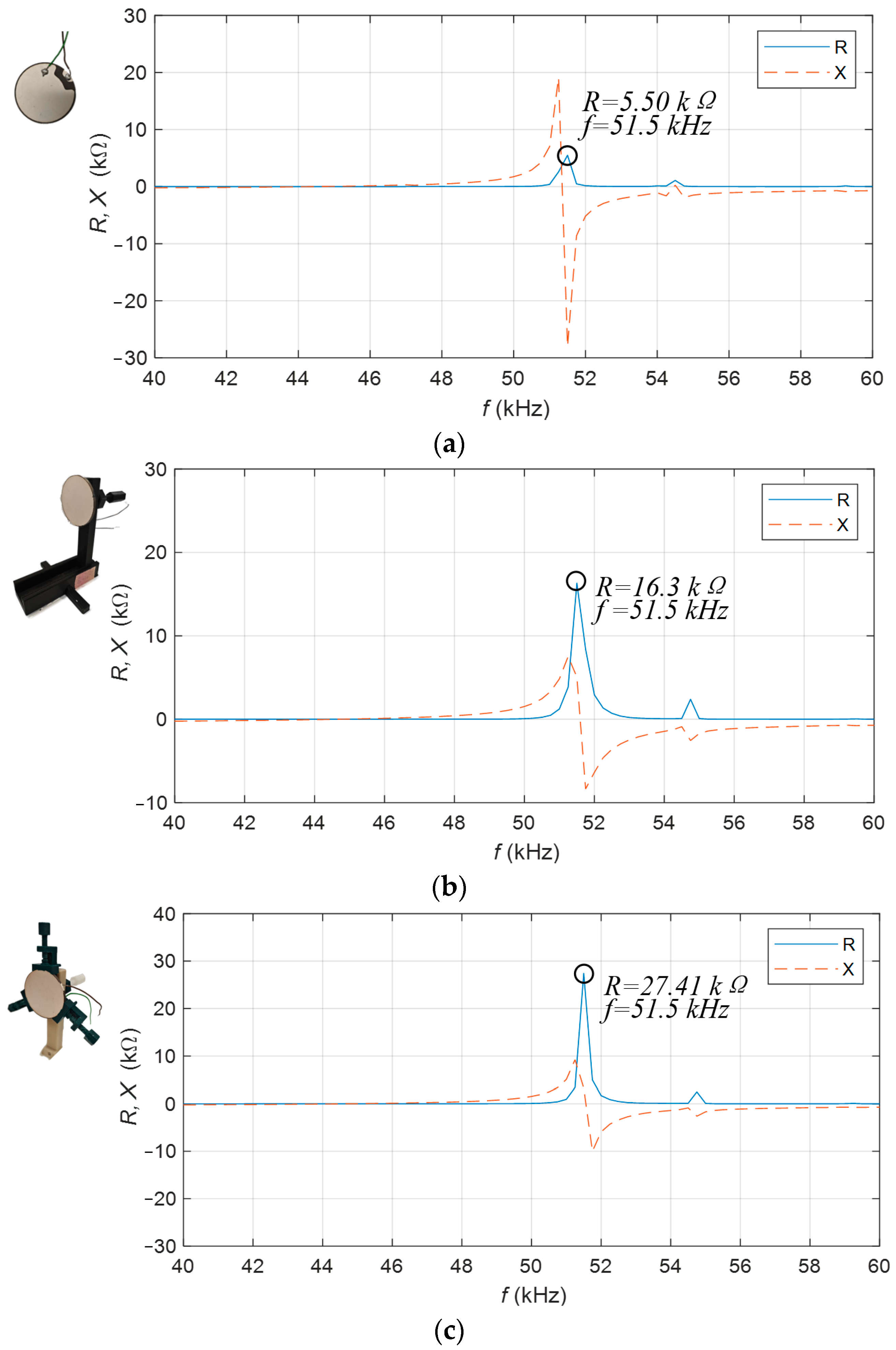
3.2.1. Impedance Characteristics
3.2.2. Distance Characteristics
4. Conclusions
Author Contributions
Funding
Institutional Review Board Statement
Informed Consent Statement
Data Availability Statement
Conflicts of Interest
References
- Rim, C.T.; Mi, C. Wireless Power Transfer for Electric Vehicles and Mobile Devices; John Wiley & Sons: New York, NY, USA, 2017. [Google Scholar]
- Hui, S.Y.R.; Zhong, W.; Lee, C.K. A critical review of recent progress in mid-range wireless power transfer. IEEE Trans. Power Electron. 2013, 29, 4500–4511. [Google Scholar] [CrossRef]
- Bhardwaj, A.; Allam, A.; Erturk, A.; Sabra, K.G. Enhancing underwater Acoustic Identification Tag design using concurrent wireless ultrasonic power transfer and backscatter communication. J. Acoust. Soc. Am. 2022, 152, A214. [Google Scholar] [CrossRef]
- Roes, M.G.; Duarte, J.L.; Hendrix, M.A.; Lomonova, E.A. Acoustic energy transfer: A review. IEEE Trans. Ind. Electron. 2012, 60, 242–248. [Google Scholar] [CrossRef]
- Basaeri, H.; Christensen, D.B.; Roundy, S. A review of acoustic power transfer for bio-medical implants. Smart Mater. Struct. 2016, 25, 123001. [Google Scholar] [CrossRef]
- Kim, K.; Jang, S.G.; Lim, H.G.; Kim, H.H.; Park, S.M. Acoustic Power Transfer Using Self-Focused Transducers for Miniaturized Implantable Neurostimulators. IEEE Access 2021, 9, 153850–153862. [Google Scholar] [CrossRef]
- Turner, B.L.; Senevirathne, S.; Kilgour, K.; McArt, D.; Biggs, M.; Menegatti, S.; Daniele, M.A. Ultrasound-Powered Implants: A Critical Review of Piezoelectric Material Selection and Applications. Adv. Healthc. Mater. 2021, 10, 2100986. [Google Scholar] [CrossRef]
- Zaid, T.; Saat, S.; Jamal, N.; Husin, S.H.; Yusof, Y.; Nguang, S. A development of acoustic energy transfer system through air medium using push-pull power converter. WSEAS Trans. Power Syst. 2016, 11, 35–42. [Google Scholar]
- Freychet, O.; Frassati, F.; Boisseau, S.; Garraud, N.; Gasnier, P.; Despesse, G. Analytical optimization of piezoelectric acoustic power transfer systems. Eng. Res. Express 2020, 2, 045022. [Google Scholar] [CrossRef]
- Zhou, J.; Bai, J.; Liu, Y. Fabrication and modeling of matching system for air-coupled transducer. Micromachines 2022, 13, 781. [Google Scholar] [CrossRef]
- Toda, M. New type of matching layer for air-coupled ultrasonic transducers. IEEE Trans. Ultrason. Ferroelectr. Freq. Control. 2002, 49, 972–979. [Google Scholar] [CrossRef]
- Kelly, S.P.; Hayward, G.; Álvarez-Arenas, T.G. Characterization and assessment of an integrated matching layer for air-coupled ultrasonic applications. IEEE Trans. Ultrason. Ferroelectr. Freq. Control. 2004, 51, 1314–1323. [Google Scholar] [CrossRef]
- Alvarez-Arenas, T.G. Acoustic impedance matching of piezoelectric transducers to the air. IEEE Trans. Ultrason. Ferroelectr. Freq. Control. 2004, 51, 624–633. [Google Scholar] [CrossRef]
- Gomez Alvarez-Arenas, T.E. Air-coupled piezoelectric transducers with active polypropylene foam matching layers. Sensors 2013, 13, 5996–6013. [Google Scholar] [CrossRef] [PubMed]
- Saito, K.; Nishihira, M.; Imano, K. Experimental Study on Intermediate Layer for Air-Coupled Ultrasonic Transducer with (0-3) Composite Materials. Proc. Symp. Ultrason. Electron 2006, 27, 213–214. [Google Scholar] [CrossRef]
- Bovtun, V.; Döring, J.; Bartusch, J.; Beck, U.; Erhard, A.; Yakymenko, Y. Ferroelectret non-contact ultrasonic transducers. Appl. Phys. A 2007, 88, 737–743. [Google Scholar] [CrossRef]
- Kazys, R.J.; Sliteris, R.; Sestoke, J. Air-coupled low frequency ultrasonic transducers and arrays with PMN-32% PT piezoelectric crystals. Sensors 2017, 17, 95. [Google Scholar] [CrossRef] [PubMed]
- Kazys, R.; Sliteris, R.; Sestoke, J.; Vladisauskas, A. Air-coupled Ultrasonic Transducers based on an Application of the PMN-32% PT Single Crystals. Ferroelectrics 2015, 480, 85–91. [Google Scholar] [CrossRef]
- Li, Y.; Yu, G.; Liang, B.; Zou, X.; Li, G.; Cheng, S.; Cheng, J. Three-dimensional ultrathin planar lenses by acoustic metamaterials. Sci. Rep. 2014, 4, 6830. [Google Scholar] [CrossRef]
- Zhu, Y.; Fan, X.; Liang, B.; Cheng, J.; Jing, Y. Ultrathin acoustic metasurface-based Schroeder diffuser. Phys. Rev. X 2017, 7, 021034. [Google Scholar] [CrossRef]
- Kim, J.; Park, S.; Anzan-Uz-Zaman, M.; Song, K. Holographic acoustic admittance surface for acoustic beam steering. Appl. Phys. Lett. 2019, 115, 193501. [Google Scholar] [CrossRef]
- Bok, E.; Park, J.J.; Choi, H.; Han, C.K.; Wright, O.B.; Lee, S.H. Metasurface for water-to-air sound transmission. Phys. Rev. Lett. 2018, 120, 044302. [Google Scholar] [CrossRef] [PubMed]
- Yang, T.; Lin, Z.; Yang, T. Experimental Evidence of High-Efficiency Nonlocal Waterborne Acoustic Metasurfaces. Adv. Eng. Mater. 2023, 25, 2200805. [Google Scholar] [CrossRef]
- Leung, H.F.; Hu, A.P. Modeling the contact interface of ultrasonic power transfer system based on mechanical and electrical equivalence. IEEE J. Emerg. Sel. Top. Power Electron. 2017, 6, 800–811. [Google Scholar] [CrossRef]
- Tseng, V.F.G.; Radice, J.J.; Drummond, T.E.; Goodrich, S.; Diamond, D.; Lazarus, N.; Bedair, S.S. Self-detachable through-metal acoustic wireless power transfer. IEEE Trans. Ultrason. Ferroelectr. Freq. Control. 2022, 69, 2381–2389. [Google Scholar] [CrossRef] [PubMed]
- Shatalov, M.; Marais, J.; Fedotov, I.; Tenkam, M.D.; Schmidt, M. Longitudinal vibration of isotropic solid rods: From classical to modern theories. Adv. Comput. Sci. Eng. 2011, 1877, 187–216. [Google Scholar]
- Fedotov, I.A.; Polyanin, A.D.; Shatalov, M.Y. Theory of Free and Forced Vibrations of a Rigid Rod Based on the Rayleigh Model. Dokl. Phys. 2007, 52, 607–612. [Google Scholar] [CrossRef]
- Bishop, R.E.D. Longitudinal Waves in Beams. Aeronaut. Q. 1952, 3, 280–293. [Google Scholar] [CrossRef]
- Allam, A.; Sabra, K.; Erturk, A. Comparison of various models for piezoelectric receivers in wireless acoustic power transfer. In Proceedings of the Active and Passive Smart Structures and Integrated Systems XIII, Denver, CO, USA, 27 March 2019; Volume 10967, pp. 198–205. [Google Scholar]
- Mason, W.P. An electromechanical representation of a piezoelectric crystal used as a transducer. Proc. Inst. Radio Eng. 1935, 23, 1252–1263. [Google Scholar]
- Mason, W.P. A dynamic measurement of the elastic, electric and piezoelectric constants of rochelle salt. Phys. Rev. 1939, 55, 775. [Google Scholar] [CrossRef]
- Wu, M.; Chen, X.; Qi, C.; Mu, X. Considering losses to enhance circuit model accuracy of ultrasonic wireless power transfer system. IEEE Trans. Ind. Electron. 2019, 67, 8788–8798. [Google Scholar] [CrossRef]
- Chubachi, N.; Kamata, H. Various equivalent circuits for thickness mode piezoelectric transducers. Electron. Commun. Jpn. Part II Electron. 1996, 79, 50–59. [Google Scholar] [CrossRef]
- Thorvaldsson, T.; Nyffeler, F.M. Rigorous derivation of the Mason equivalent circuit parameters from coupled mode theory. In Proceedings of the IEEE 1986 Ultrasonics Symposium, Williamsburg, VA, USA, 17–19 November 1986; pp. 91–96. [Google Scholar]
- Jin, P.; Fu, J.; Wang, F.; Zhang, Y.; Wang, P.; Liu, X.; Feng, X. A flexible, stretchable system for simultaneous acoustic energy transfer and communication. Sci. Adv. 2021, 7, eabg2507. [Google Scholar] [CrossRef] [PubMed]
- Gokhale, V.J.; Downey, B.P.; Katzer, D.S.; Hardy, M.T.; Nepal, N.; Meyer, D.J. Engineering efficient acoustic power transfer in HBARs and other composite resonators. J. Microelectromech. Syst. 2020, 29, 1014–1019. [Google Scholar] [CrossRef]
- Bakhtiari-Nejad, M.; Hajj, M.R.; Shahab, S. Dynamics of acoustic impedance matching layers in contactless ultrasonic power transfer systems. Smart Mater. Struct. 2020, 29, 035037. [Google Scholar] [CrossRef]
- Song, K.; Kwak, J.H.; Park, J.J.; Hur, S. Acoustic metasurfaces for efficient matching of non-contact ultrasonic transducers. Smart Mater. Struct. 2021, 30, 085011. [Google Scholar] [CrossRef]


| Medium | Acoustic Impendence | Density | Sound Speed |
|---|---|---|---|
| Steel | 39 × 106 | 7700 | 5000 |
| Aluminium | 14 × 106 | 2700 | 5200 |
| Water | 1.44 × 10⁶ | 1000 | 1440 |
| Air | 410 | 1.2 | 340 |
| PZT-5H | 36 × 106 | 7500 | 4800 |
| Material Properties | Symbol | Meaning | |
|---|---|---|---|
| Density | |||
| t | Thickness | ||
| Permittivity | |||
| Electromechanical coupling | |||
| A | Area | ||
| Elastic stiffness | |||
| Method | Ref | Medium | Power/Sound | Detachable | |
|---|---|---|---|---|---|
| Author | Year | ||||
| Special material | [9] Freychet 2020 | Wall | Power | Non-detachable | |
| [10] Zhou 2022 | Air | Power | Non-detachable | ||
| [17] Rymantas 2017 | Air | Sound | Detachable | ||
| Metasurface | [22] Eun 2018 | Air/water | Sound | Detachable | |
| Clamp | [25] Tseng 2022 | Metal | Power | Detachable | |
| This Research | Air | Power | Detachable | ||
| Boundary | Mechanical Status | Electrical Status |
|---|---|---|
| A | Axisymmetric | Axisymmetric |
| B | Free | Terminal Voltage |
| C | Free | Ground |
| D | Roller Support | Zero Charge |
| Physical Quantity | Unit |
|---|---|
| p (Sound pressure) | Pa |
| Lp (Sound pressure level) | dB |
| I (Sound intensity) | W/m2 |
| P (Sound power) | W |
| T (Stress) | Pa |
Disclaimer/Publisher’s Note: The statements, opinions and data contained in all publications are solely those of the individual author(s) and contributor(s) and not of MDPI and/or the editor(s). MDPI and/or the editor(s) disclaim responsibility for any injury to people or property resulting from any ideas, methods, instructions or products referred to in the content. |
© 2023 by the authors. Licensee MDPI, Basel, Switzerland. This article is an open access article distributed under the terms and conditions of the Creative Commons Attribution (CC BY) license (https://creativecommons.org/licenses/by/4.0/).
Share and Cite
Liu, L.; Abdulla, W. Improving APT Systems’ Performance in Air via Impedance Matching and 3D-Printed Clamp. Sensors 2023, 23, 5347. https://doi.org/10.3390/s23115347
Liu L, Abdulla W. Improving APT Systems’ Performance in Air via Impedance Matching and 3D-Printed Clamp. Sensors. 2023; 23(11):5347. https://doi.org/10.3390/s23115347
Chicago/Turabian StyleLiu, Liu, and Waleed Abdulla. 2023. "Improving APT Systems’ Performance in Air via Impedance Matching and 3D-Printed Clamp" Sensors 23, no. 11: 5347. https://doi.org/10.3390/s23115347
APA StyleLiu, L., & Abdulla, W. (2023). Improving APT Systems’ Performance in Air via Impedance Matching and 3D-Printed Clamp. Sensors, 23(11), 5347. https://doi.org/10.3390/s23115347