Dynamic Evaluation of the Degradation Process of Vibration Performance for Machine Tool Spindle Bearings

Abstract

Real-time condition monitoring and fault diagnosis of spindle bearings are critical to the normal operation of the matching machine tool. In this work, considering the interference of random factors, the uncertainty of the vibration performance maintaining reliability (VPMR) is introduced for machine tool spindle bearings (MTSB). The maximum entropy method and Poisson counting principle are combined to solve the variation probability, so as to accurately characterize the degradation process of the optimal vibration performance state (OVPS) for MTSB. The dynamic mean uncertainty calculated using the least-squares method by polynomial fitting, fused into the grey bootstrap maximum entropy method, is utilized to evaluate the random fluctuation state of OVPS. Then, the VPMR is calculated, which is used to dynamically evaluate the failure degree of accuracy for MTSB. The results show that the maximum relative errors between the estimated true value and the actual value of the VPMR are 6.55% and 9.91%, and appropriate remedial measures should be taken before 6773 min and 5134 min for the MTSB in Case 1 and Case 2, respectively, so as to avoid serious safety accidents that are caused by the failure of OVPS.

1. Introduction

Precision, as one of the most important performance indicators of spindle bearings, has a significant impact on the normal operation of machine tools. Super-precision spindle bearings (SPSB) refer to spindle bearings with low vibration, a wide speed range, a high rotational accuracy, low heating, high system rigidity, and low noise. SPSB works at the OVPS, which is the basis for a machine tool to achieve optimal performance. The failure of MTSB are not only due to fatigue. A variety of performance failures, such as stuck, sintering, plastic deformation, crack, or fracture may occur before fatigue failure [1,2,3]. The probability distribution of these failure modes is unknown, and the characteristic data of the spindle bearings are scarce. In particular, the non-linear dynamic contact and collision between the parts inside the spindle bearings, the non-linear damage, viscous-temperature and viscous-pressure characteristics of lubricating medium, and the accuracy loss, all present uncertain and non-linear characteristics [4,5,6,7]. These uncertainties bring new challenges to analyze the degradation trend of vibration performance. Therefore, it is of great significance to evaluate the degradation process of vibration performance dynamically before the MTSB fail.

When analyzing the degradation process of bearings, the mathematical statistical methods generally assume that the amount of data are limited, and then extract characteristic parameters of bearings [8,9,10]. Based on the vibration signal collected, Ye et al. [11] used the maximum entropy method to calculate the PDF of bearings, which was regarded as degradation characteristics. Then, the Bayesian method, the bootstrap method and the maximum entropy method were fused to evaluate the reliability of bearings in service. Its performance degradation and reliability evaluation process are shown in Figure 1.

Figure 1. Performance degradation and reliability evaluation process of rolling bearings.

However, due to the differences of experimental data samples caused by random factors and interference factors in the experimental process, or the incompleteness of information of data samples, it is difficult to represent the entire distribution range of bearing life accurately. For two sets of bearings with the same batch and model, the prediction results may also be different, that is, the generalization ability and stability of the model cannot be guaranteed. In order to reduce the impact of random and interfering factors on the analysis results, many experts and scholars at home and abroad preprocess the experimental data. Huang et al. [12] fused empirical mode decomposition method and Hilbert transform method to analyze the time-frequency spectrum of signals, making up for the shortcomings of traditional statistical theory in analyzing nonlinear and non-stationary data. In order to avoid multiple spline curve fitting in the process of empirical mode decomposition, Feldman [13] proposed a time-varying vibration decomposition method based on Hilbert transform. In order to not affect the accuracy of condition monitoring and fault diagnosis, Guo et al. [14] proposed a signal compression method based on integrated empirical mode decomposition, which adaptively decomposes the vibration signal into signal components with different frequency bands. These preprocessing methods may reduce the influence of random and interference factors, while also filtering out some useful information, resulting in “distortion” of the analysis results, which in turn leads to the inability to evaluate the degradation process of bearings effectively.

Traditional machine learning and deep learning, as methods widely used in data preprocessing, have their own advantages and disadvantages. In the field of traditional machine learning, SVM has a low error rate of generalization, a low computational overhead, and it is easy to interpret its results [15,16]. However, SVM is too sensitive to parameters of kernel functions. The idea of KNN is simple, with no assumptions about data input, but its disadvantage is that the computational complexity is high [17]. The logistic regression method has low computational cost, and it is easy to understand and implement [18]. However, it is prone to underfitting and its classification accuracy is not high. The decision tree is insensitive to missing intermediate values, and can handle irrelevant feature data [19]. It is better than KNN in understanding the inherent meaning of the data. Its disadvantage is that it is prone to overfitting and the construction process is time-consuming.

Deep learning and traditional machine learning are similar in data preprocessing. The core difference lies in the feature extraction process, where deep learning does not require manual extraction and the extraction process is performed by a machine [20,21,22,23]. Although deep learning can learn the features of patterns automatically and achieve high recognition accuracy, the prerequisite is that amounts of data are provided. For a limited amount of data, deep learning algorithms cannot estimate the laws of data without bias. The weight parameters of CNN are less than those of DNN connected fully, which makes the training speed of CNN model faster and is not prone to overfitting [24]. Meanwhile, CNN requires less data to train. The disadvantage is that it requires large sample size and parameter adjustment, and its physical meaning is also unclear. RNN cannot solve the problem of long-term dependence, while LSTM implements temporal memory function and prevents gradient disappearance. At the same time, LSTM can better handle the tasks of time series than CNN. In addition, it also solves the long-term dependency problem [25,26,27]. However, the model structure of LSTM is complex relatively, and its training process is more time-consuming than CNN. The characteristics of RNNs determine that they cannot parallelize data well. It is also difficult for LSTM to handle longer data sequences.

Vibration data collected through the experiment vary with time, which can be regarded as a non-linear time series. From the beginning of service to the failure of accuracy, the vibration performance varies continuously, forming multiple time series. The intrinsic series refers to the time series with OPS. According to the time series of MTSB, the degradation process of accuracy is defined as a Poisson process, and the degradation probability is taken as a parameter of the counting process [28]. Influenced by many factors, the degradation process of bearings has the characteristics of non-linear dynamics [29,30]. For each time series of accuracy, the degradation probability relative to the intrinsic series also has the characteristics of non-linearity and diversity. This causes a dynamic change in information. In particular, the degradation probability functions of accuracy vary with time and environmental factors. In view of this, a polynomial is used to fit the parameters, and the data samples of the degradation probability of OVPS are obtained for each time series. Since it is difficult to obtain enough original information of degradation probability in a short time, the grey bootstrap method is used to generate a large set of sample data [31].

Information fusion technology and the real-time update method can improve the prediction accuracy, but most of the existing fusion methods focus on the fusion of homogeneous information collected by the sensors with same type. They rarely consider the fusion of heterogeneous information, especially the fusion and prediction of event single value data and waveform data monitored, which needs further in-depth study [32,33]. In addition, the current real-time update methods basically take Bayesian method as the theoretical framework. They can only apply the observed data to update the priori probability distribution, but cannot utilize other available information such as moments of parameters or functions of moments.

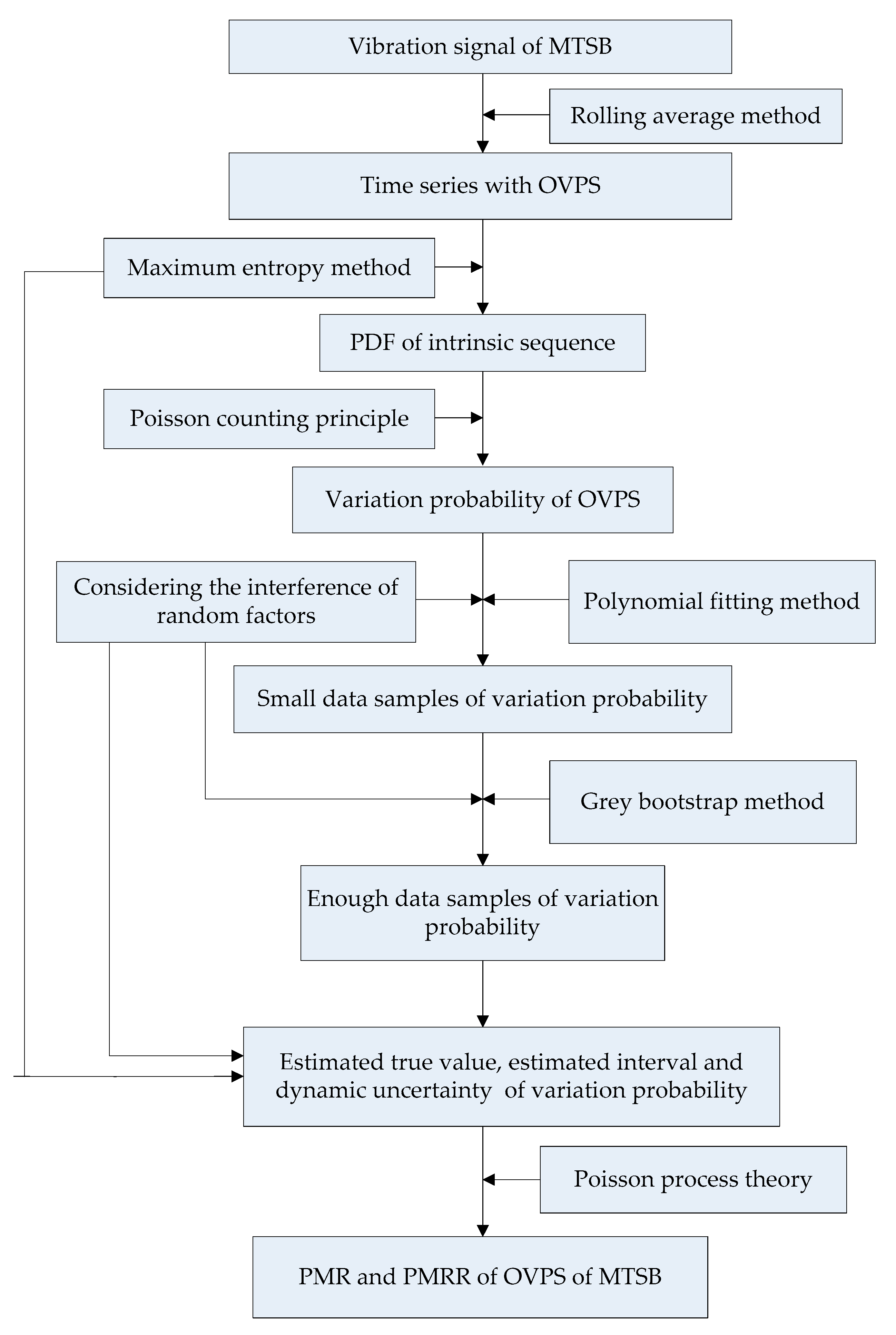
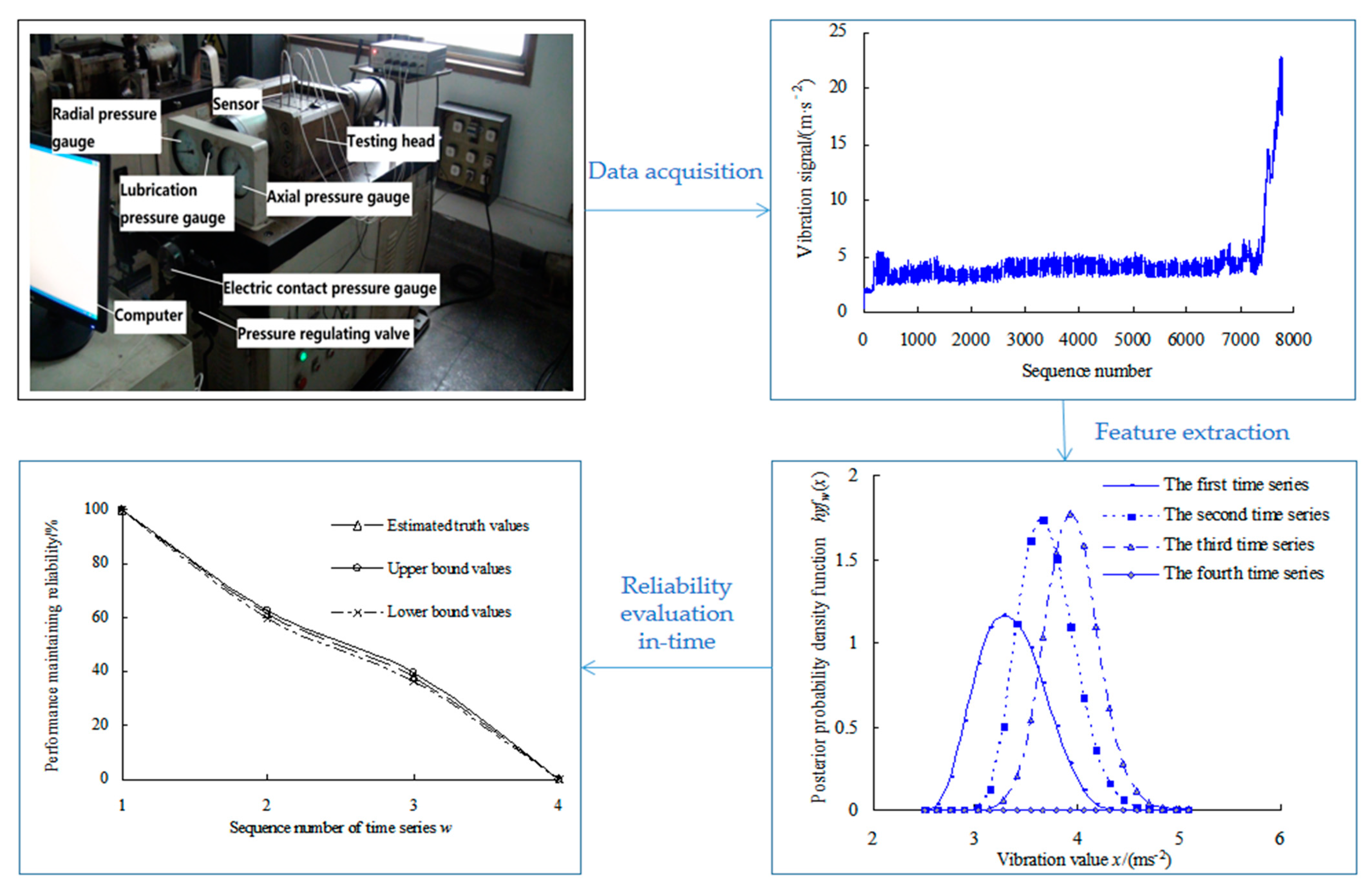
On the basis of this, a dynamic evaluation model is established to study the performance degradation process for MTSB. This model considers the interference of random factors during the service process of MTSB. First, the vibration signal are processed into segments to obtain the time series with OVPS based on rolling average method. The maximum entropy method is used to calculate the PDF of intrinsic sequence. Based on the Poisson counting principle, the variation probabilities of OVPS of each time series are calculated. Considering the interference of random factors, the small data sample of variation probability is obtained for each time series by polynomial fitting method. The grey bootstrap method (namely, GBM (1,1)) is applied to generate enough data samples of variation probability, so as to obtain the estimated true value, estimated interval and dynamic uncertainty of variation probability. The PMR and PMRR of OVPS of MTSB are calculated according to Poisson process theory. Experimental verification is utilized to verify that the proposed model can be used effectively to estimate the failure degree of OVPS to monitor and analyze the performance degradation process of MTSB.

The flow diagram of proposed method is shown in Figure 2.

Figure 2. Flow diagram of proposed method.

2. Mathematical Models

Based on the maximum entropy method and the Poisson counting principle, the variation probability of the OVPS is calculated for MTSB. The small data sample of variation probability is obtained by polynomial fitting for each time series. The estimated true value curve and the upper- and lower-bound curves of variation probability are obtained by fusing the grey bootstrap method into the maximum entropy method. The VPMR is calculated based on the Poisson process, which is used to dynamically evaluate the failure degree of OVPS for MTSB.

2.1. Calculating Variation Probability of OVPS

During the service period of the spindle bearings, r time sequences are obtained by periodic sampling vibration acceleration signals of spindle bearings. The time series collected after initially wearing is considered to be the intrinsic sequence, which is marked as the first time series and expressed by the vector X₁ as

$${\mathit{X}}_1=(x(1),x(2),\dots ,x(k),\dots ,x(N)).$$

(1)

where x(k) is kth performance data in the intrinsic sequence; k is the order number of performance data in intrinsic sequence, k = 1, 2, 3, …, N; N is the total number of performance data in the intrinsic sequence.

With the change of time variable, vibration acceleration data are collected continuously, and the nth time series vector X_n is obtained.

$${\mathit{X}}_n=(x_n(1),x_n(2),\dots ,x_n(k),\dots ,x_n(N)).$$

(2)

where x_n(k) is the kth performance data of the nth time series; n is the order number of time series, n = 1, 2, 3, …, r.

The maximum entropy method can make the optimal estimation for the unknown probability distribution with minimal subjective bias. Lagrange multipliers are introduced in the process of solving probability distributions, so the problem of solving probability distribution is transformed into the problem of solving Lagrange multipliers. For the convenience of description, the continuous variable x is used to express the discrete variable x(k) in the intrinsic sequence.

According to the maximum entropy method, the probability density function should meet the condition that the value of entropy function H(x) is the maximum.

$$H(x)=-{\displaystyle \underset{S}{\int }f\left(x\right)\ln f\left(x\right)}\mathrm{d}x$$

(3)

where f(x) is the probability density function of continuous variable x; lnf(x) is the logarithm of the probability density function f(x); S is the feasible domain of the performance random variable x, S = [S₁, S₂]; S₁ is the lower-bound value of the feasible domain, and S₂ is the upper-bound value of the feasible domain.

Then, the Lagrange multiplier method is used to solve this problem by adjusting the probability density function f(x) to maximize the value of entropy function H(x) [11]. Assume H is the Lagrange function.

$$\overline{H}=H(x)+(c_0+1\left)\right[{\displaystyle \underset{S}{\int }f\left(x\right)}\mathrm{d}x-1]+{\displaystyle \sum _{i=1}^j{c}_i[}{\displaystyle \underset{S}{\int }{x}^{i}f\left(x\right)}\mathrm{d}x-m_i]$$

(4)

where i is the order number of origin moment, i = 1, 2, …, j, usually j = 5; m_i is the ith order origin moment, m₀ = 1; xⁱ is the coefficient of the function f(x); c_i is the (i + 1)th Lagrange multiplier and c₀ is the first Lagrange multiplier, i = 1, 2, …, j.

The probability density function f(x) of data samples can be expressed as

$$f(x)=\exp (c_0+{\displaystyle \sum _{i=1}^j{c}_i{x}^i})$$

(5)

With

$$c_0=-\ln ({\displaystyle \underset{S}{\int }\exp ({\displaystyle \sum _{i=1}^j{c}_i{x}^i})}\mathrm{d}x)$$

(6)

The other j Lagrange multipliers should satisfy that

$$1-\frac{{\displaystyle \underset{S}{\int }{x}^i\exp ({\displaystyle \sum _{i=1}^j{c}_i{x}^i})}\mathrm{d}x}{m_i{\displaystyle \underset{S}{\int }\exp ({\displaystyle \sum _{i=1}^j{c}_i{x}^i})}\mathrm{d}x}=0$$

(7)

To ensure the convergence of solution, the original data interval is mapped to interval [−e, e] by the substitution of variable. The sample data are divided into ξ groups in the incremental order, and the histogram can be drawn. At the same time, the values z_μ and frequency Γ_μ can be calculated, and u = 2, 3, …, ξ + 1. Then, the histogram is extended into (ξ + 2) group and let Γ₁ = Γ_ξ+2.

Let

$$\psi =ax+b$$

(8)

where ψ is the variable to be transformed, ψ ∈ [−e, e]; a and b are the mapping parameters; e has a value of 2.71828.

$$x=\frac{\psi -b}{a}$$

(9)

The mapping parameters a and b can be calculated based on dx = dψ/a.

$$a=\frac{2\mathrm{e}}{z_{\xi +2}-z_1}$$

(10)

$$b=\mathrm{e}-a{z}_{\xi +2}$$

(11)

Therefore, the probability density function f(x) can be transformed into

$$f(x)=\exp [c_0+{\displaystyle \sum _{i=1}^j{c}_i{(ax+b)}^i}\left)\right]$$

(12)

Set a significant level α, α ∈ [0, 1], so the confidence level P is given by

$$\alpha =(1-P)\times 100\%$$

(13)

The maximum entropy estimated interval is [X_L, X_U] for a given confidence level P, and the lower-bound value X_L should meet that X_L = X_α/2.

And

$$\frac{1}{2}\alpha ={\displaystyle {\int }_{S_1}^{{\mathit{X}}_{\mathrm{L}}}f\left(x\right)}\mathrm{d}x$$

(14)

The upper-bound value should meet that X_U = X_(1−α)/2. And

$$\frac{1}{2}\alpha ={\displaystyle {\int }_{X_{\mathrm{U}}}^{S_2}f\left(x\right)}\mathrm{d}x$$

(15)

So the maximum entropy estimated interval for continuous variable x can be given by

$$\left[X_L,X_U\right]=[X_{\frac{\alpha }{2}},X_{1-\frac{\alpha }{2}}]$$

(16)

According to Equation (16), the maximum entropy estimated interval [X_L1, X_U1] can be calculated for the intrinsic time series, where X_L1 is the lower-bound value and X_U1 is the upper-bound value of the maximum entropy estimated interval of the intrinsic time series.

Based on the Poisson counting principle, record the number N_n that performance data of the nth time series is outside the estimated interval [X_L1, X_U1]. Then, the variation frequency λ_n can be given as Equation (17) for the nth time series.

$${\lambda }_n=\frac{N_n}{N}$$

(17)

With

$$N_n=N_{n1}+N_{n2}.$$

(18)

where N_n1 is the number showing that performance data are less than X_L1 for the nth time series; N_n2 is the number showing that performance data are more than X_U1 for the nth time series; n is the sequence number of time series, n = 1, 2, 3, …, r.

2.2. Calculating Estimated Truth Value and Estimated Interval of Variation Probability

The least-squares method is used to fit the variation probability with different order polynomials. The fitting effect depends on the correlation coefficient R². The closer the correlation coefficient R² is to 1, the better the polynomial fitting effect. If the correlation coefficient R² is less than 0.8, the fitting effect is worse, so the polynomial will not be used in the later analysis process.

The polynomial function G_q(λ) is given by

$$G_q\left(\lambda \right)=p_{q0}{\lambda }^0+p_{q1}{\lambda }^1+p_{q2}{\lambda }^2\dots +p_{q\gamma }{\lambda }^{\gamma }+\dots +p_{qq}{\lambda }^q;\gamma =0,1,2,\dots ,q;q=1,2,\dots ,6;$$

(19)

where G_q(λ) is the qth order polynomial; q is the order number of polynomial function; p_qγ is the coefficient of the power function λ^γ.

According to the above polynomial function models, small data samples of variation probability of OVPS are obtained for each time series.

$$\mathit{Y}\left(n\right)=\left(y_n\left(1\right),y_n\left(2\right),\dots ,y_n\left(6\right)\right)=\left(y_n\left(u\right)\right);u=1, 2,\dots ,6;n=1,2,\dots ,r;$$

(20)

where Y(n) is the data sample of variation probability of OVPS for the n time series; y_n(u) is the uth data in the variation probability data sample for the n time series.

Using the bootstrap method, B bootstrap re-sampling samples of size z, namely the bootstrap re-sampling samples V_Bootstrap, can be obtained by an equiprobable sampling as

$${\mathit{V}}_{\mathrm{Bootstrap}}=\left({\mathit{V}}_1,{\mathit{V}}_2,\dots ,{\mathit{V}}_{\beta },\dots ,{\mathit{V}}_B\right)$$

(21)

where V_β is the βth bootstrap re-sampling sample, β = 1, 2, …, B; B is the times of the bootstrap re-sampling, and also the number of bootstrap samples, with

$${\mathit{V}}_{\beta }=\left[v_{\beta }(\mathrm{\Theta })\right];\mathrm{\Theta }=1,2,\dots ,z$$

(22)

where v_β(Θ) is the Θth data in the βth bootstrap re-sampling sample.

According to the grey model GM (1,1) [34], suppose the first-order accumulated generating operator (1-AGO) of V_β is given by

$${\mathit{Y}}_{\beta }=\left[y_{\xi \beta }\left(u\right)\right]={\displaystyle \sum _{j=1}^{\mathrm{\Theta }}{v}_{\xi \beta }\left(j\right)}$$

(23)

The grey generated model can be described as the differential equation as follows:

$$\frac{\mathrm{d}{y}_{\xi \beta }\left(u\right)}{\mathrm{d}u}+c_1{y}_{\xi \beta }\left(u\right)=c_2$$

(24)

where u is the time variable, and c₁ and c₂ are the coefficients to be estimated.

Use the increment to replace the differential, viz.,

$$\frac{\mathrm{d}{y}_{\xi \beta }\left(u\right)}{\mathrm{d}u}=\frac{\Delta y_{\xi \beta }\left(u\right)}{\Delta u}=y_{\xi \beta }\left(u+1\right)-y_{\xi \beta }\left(u\right)=v_{\xi \beta }\left(u+1\right)$$

(25)

where Δu is equal to the unit interval, 1. Furthermore, assume the generated vector of the mean series as follows

$$Z_{\beta }=\left[z_{\beta }\left(u\right)\right]=\left[0.5y_{\xi \beta }\left(u\right)+0.5y_{\xi \beta }(u-1)\right]$$

(26)

The least-squares solution with the initial condition y_ξβ(1) = v_ξβ(1) is given by

$${\widehat{y}}_{\xi \beta }\left(z+1\right)=\left(v_{\xi \beta }\left(1\right)-c_2/c_1\right){\mathrm{e}}^{{-\mathrm{c}}_{1}z}+c_2/c_1$$

(27)

where the coefficients c₁ and c₂ are as follows

$${\left(c_1,c_2\right)}^{\mathrm{T}}={\left({\mathit{D}}^{\mathrm{T}}\mathit{D}\right)}^{-1}{\mathit{D}}^{\mathrm{T}}{\left({\mathit{V}}_{\beta }\right)}^{\mathrm{T}}$$

(28)

with

$$\mathit{D}={\left(-{\mathit{Z}}_{\beta },\mathit{I}\right)}^{\mathrm{T}}$$

(29)

$$\mathit{I}=\left(1,1,\dots ,1\right)$$

(30)

According to the inverse AGO [34], the βth generated data are expressed as

$$\widehat{\nu }\left(z+1\right)={\widehat{y}}_{\mathit{\xi }\mathit{\beta }}\left(z+1\right)-{\widehat{y}}_{\mathit{\xi }\mathit{\beta }}\left(z\right)-c$$

(31)

Therefore, B generated data for the vibration performance can be obtained as

$${\mathit{Y}}_B=\left(w_1,w_2,\dots ,w_{\mathit{\beta }},\dots ,w_B\right)=\left({\widehat{\nu }}_1\left(z+1\right),{\widehat{\nu }}_2\left(z+1\right),\dots ,{\widehat{\nu }}_{\mathit{\beta }}\left(z+1\right),\dots ,{\widehat{\nu }}_B\left(z+1\right)\right)$$

(32)

where w_β is the βth generated data.

The maximum entropy method is used to calculate the probability density function of the generated sample Y_B. According to the probability density function, the true value and upper- and lower-bound values are estimated for the data sample of variation probability of each time series.

The probability density function of variation probability data sample can be calculated as

$$f({\lambda }_n)=\exp [c_{0n}+{\displaystyle \sum _{i=1}^j{c}_{in}{(a_n{\lambda }_n+b_n)}^i}\left)\right]$$

(33)

The estimated true value of the variability probability is obtained as

$${\lambda }_{n0}={\displaystyle \underset{S}{\int }{\lambda }_{n}f\left({\lambda }_n\right)}\mathrm{d}{\lambda }_n$$

(34)

Set a significant level and let α ∈ (0, 1). The maximum entropy estimated interval is given as

$$[{\lambda }_{n\mathrm{L}},{\lambda }_n{}_{\mathrm{U}}]=[{\lambda }_n{}_{\frac{\alpha }{2}},{\lambda }_n{}_{{{}_{1-}}_{\frac{\alpha }{2}}}]$$

(35)

where λ_nL is the lower-bound value and λ_nU is the upper-bound value of the variation probability data sample for the nth time series.

2.3. Evaluation of the Uncertainty of Variation Probability

The fluctuation range of variation probability can be expressed as

$$U_{\lambda }{}_{{}_n}={\lambda }_n{}_{\mathrm{U}}-{\lambda }_n{}_{\mathrm{L}}$$

(36)

where U_λn is the estimated uncertainty of variation probability, namely, the instantaneous uncertainty at the confidence level P.

The number η is calculated for variation probability sample data more than the upper-bound value λ_nU based on the Poisson counting process, and the reliability of evaluation result is defined as

$$P_R=\left(1-\eta /r\right)\times 100\%$$

(37)

where P_R is the reliability of the polynomials fitting effect using the least-squares method.

Define

$$U_{\mathrm{mean}}=\left(1/r\right){\displaystyle \sum _{n=1}^r{U}_{{\lambda }_n}}|{}_{P_R=100\%}$$

(38)

where U_mean is the dynamic average uncertainty; |_PR=100% stands for that the calculation process is under the condition of P_R = 100% [9].

2.4. Evaluation of PMR and PMRR

Any counting process can be described by the Poisson process [28] as

$$Q=\exp (-\theta \xi )\frac{{(\theta \xi )}^e}{e!}$$

(39)

where ξ stands for the time variable with ξ = 1, 2, 3, …, and ξ ≥ 1; e is the number of occurring failure events with e = 0, 1, 2, 3, …, namely, the serious variation in working condition that may cause the OVPS failure; Q is the probability of failure events occurring e times. Thus, the reliability R for events occurring can be obtained by the Poisson process.

When solving for the PMR of bearings working at the OVPS, let e = 0, viz., which indicates that R is the probability before the OVPS fails. Let ξ = 1, which indicates that R is the PMR of time series in current time. According to Equation (40), PMR can be expressed as

$$R\left({\lambda }_n\right)=\exp \left(-{\lambda }_n\right)$$

(40)

where R(λ_n) is a function of the variation probability λ_n.

The upper- and lower-bound values of variation probability are applied into the reliability Equation (41), so the estimated true values R₀ and upper- and lower-bound intervals [R_L, R_U] are gained for performance maintaining reliability during the time intervals corresponding to the performance time series. The range of variation probability λ_n is [0, 1]. 0 represents the OVPS of bearings without any variation, which is an ideal state and the reliability is 100% for bearing working at the OVPS. 1 represents that the OVPS of rolling bearings fail completely and the performance state is very unreliable. Therefore, if the value of λ_nL is less than 0, let λ_nL = 0 artificially in the process of solving the performance maintaining reliability.

R₀ = exp(−λ_n0), R_L = exp(−λ_nU), R_U = exp(−λ_nL)

(41)

According to the concept of relative error in measurement theory, performance maintaining relative reliability (PMRR) d(λ_n) of MTSB is obtained to characterize the failure degree of OVPS [11].

$$d\left({\lambda }_n\right)=\frac{R\left({\lambda }_n\right)-R\left({\lambda }_1\right)}{R\left({\lambda }_1\right)}\times 100\%$$

(42)

where R(λ₁) is the PMR for the intrinsic series of MTSB, R(λ_n) is the PMR for the nth time series of MTSB; d(λ_n) is the PMRR for the nth time series of MTSB.

The basic classification principle of degree failure of OVPS for MTSB is as follows:

(1)

If d(λ_n) is not less than 0%, which shows that the PMR during this period is not less than PMR of OVPS, and it cannot deny that the performance has reached its optimal state; otherwise, it can deny that the performance has achieved its optimal state.

(2)

When d(λ_n) is less than 0%, if the absolute value of d(λ_n) is in (0%, 15%], this indicates that the error between the evaluation value and the optimum value is very small. If the absolute value of d(λ_n) is in (15%, 30%], this indicates that the error between the evaluation value and the optimum value is gradually increasing. If the absolute value of d(λ_n) is greater than 30%, this indicates that the error between the evaluation value and the optimum value is very large.

Based on that, the degree failure of OVPS for MTSB is divided into S1, S2, S3, S4 for a total of four levels:

S1: If d(λ_n) ≥ 0%, it indicates the performance states of MTSB reaches the optimum and has almost no failure possibility.

S2: If d(λ_n) ∈ [−15%, 0%), it indicates the performance states of MTSB is normal, and the degree failure of OVPS is very small.

S3: If d(λ_n) ∈ [−30%, −15%), it indicates the performance states of MTSB is gradually becoming worse, and the degree failure of OVPS is gradually increasing.

S4: If d(λ_n) < −30%, it indicates the performance states of MTSB is worse, and the degree failure of OVPS is very large.

The negative value of d(λ_n) indicates the performance states has attenuation, namely, PMR currently is less than PMR during the optimum period, and the positive value indicates no attenuation. The smaller d(λ_n) is, the worse the performance states of MTSB is, and the larger the degree failure of OVPS is. Therefore, the time corresponding to d(λ_n) = −30%, is the critical time where OVPS becomes poor. Taking corresponding measures before the critical time can avoid serious safety accidents that are caused by the failure of OVPS.

3. Experimental Verification

3.1. Case 1

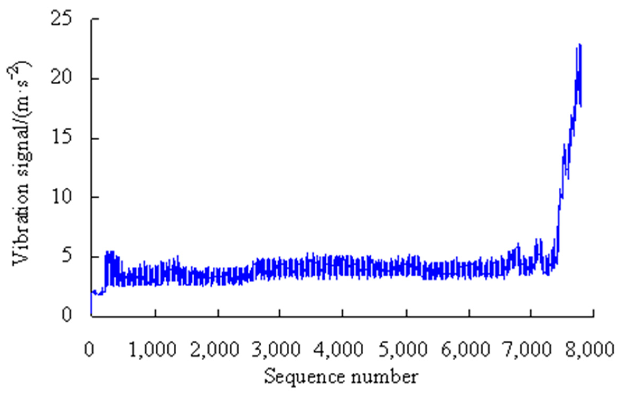
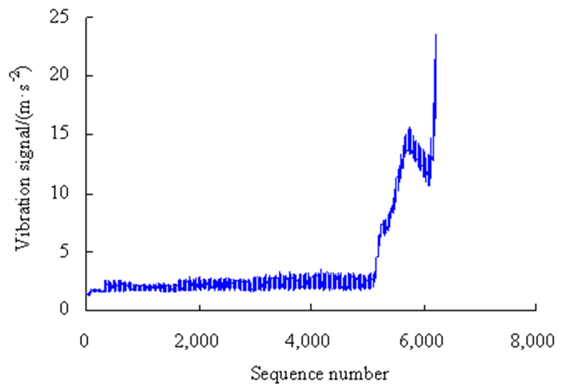
This is a strength lifetime test on the machine tool spindle bearings, which is conducted at a radial load of 4.58 kN, an axial load of 4.17 kN, and a motor speed 6000 r/min. The vibration acceleration sensor has a measuring range of ±2000 g and a resolution of 0.0001 g. The data-acquisition rate is 20 KHz. The test machine, the bearing used and the vibration data in this case are exactly the same as those of Case 1 in Reference [11]. The vibration signals are automatically collected by the computer control system, as shown in Figure 3.

Figure 3. Vibration signals of MTSB.

As shown in Figure 3, based on the rolling average method, the performance degradation stages are divided as shown in Table 1.

Table 1. Performance degradation stage divided.

Data Point	Degradation Stage
1st to 472nd	Initial wear stage
473rd to 2574th	Optimal performance state
2575th to 6659th	Normal wear stage
6660th to 7446th	Degeneration stage
7447th to 7793rd	Deterioration stage

From the OVPS of the bearing, there are 7321 vibration signals. Among them, the 473rd to 7472nd data points are divided into 10 segments at 700 data intervals. The 7473rd to 7793rd data are separated into one segment, that is, the 11th segment.

It is worth noting that if the vibration data are divided into fewer segments, the specific variation process of characteristic parameter cannot be obtained. If the vibration data are divided into a large number of segments, it will cause large computational workload and complex calculation process. At the same time, each segment of data contain less information, which makes the calculation error of the probability density function larger. Therefore, the vibration data are divided into ten segments usually in the analysis process.

3.1.1. Variation Probability of OVPS of MTSB

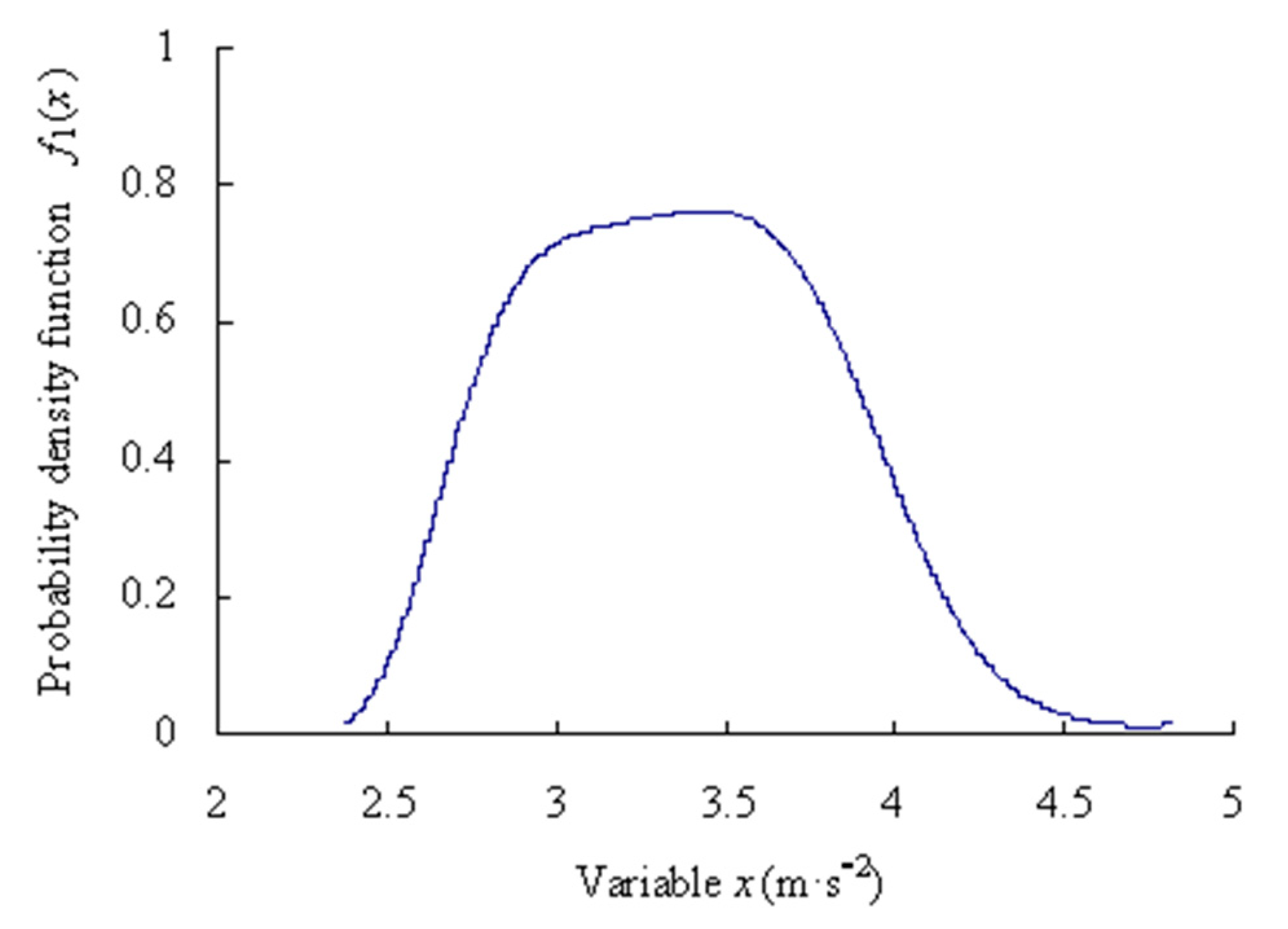
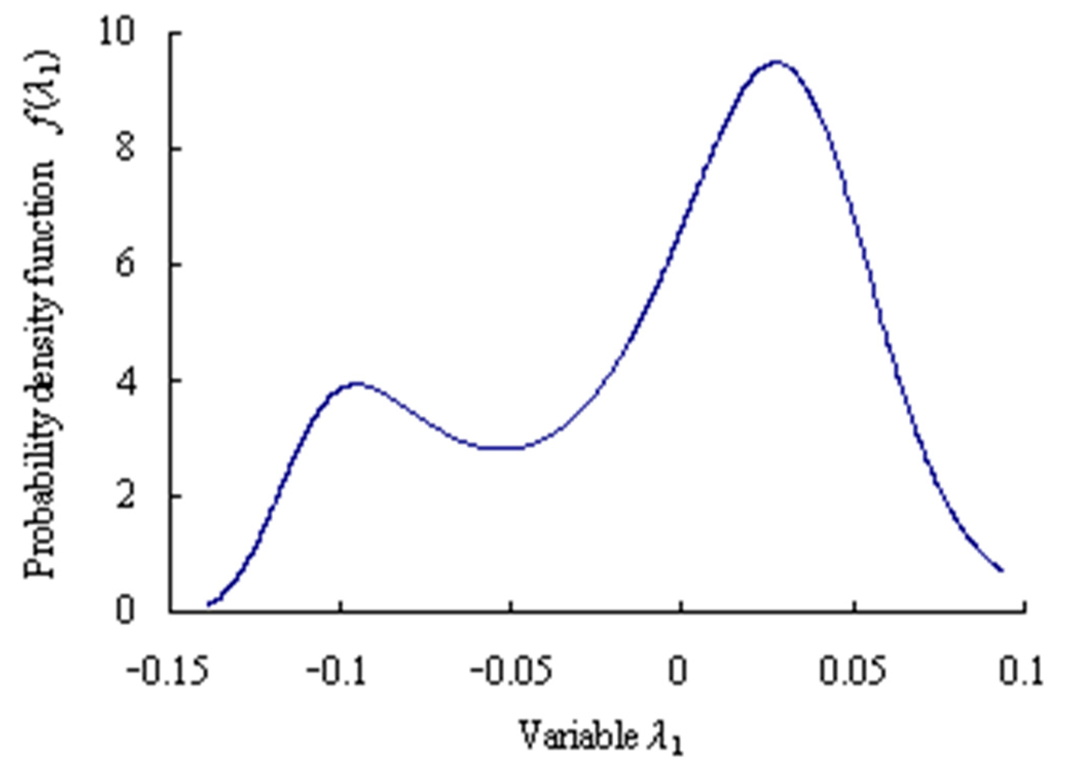
For the first time series, based on the Equations (1)–(12), the origin moments are obtained as [m₁₁, m₂₁, m₃₁, m₄₁, m₅₁] = [−0.5266, 1.2312, −1.4627, 3.5077, −5.2016]. Lagrange multipliers are calculated as [c₀₁, c₁₁, c₂₁, c₃₁, c₄₁, c₅₁] = [−0.2975, −0.1981, −0.4370, −0.2928, −0.0111, 0.0430]. Mapping parameter are gained as a₁ = 2.2241; b₁ = −8.0066. The estimated truth function f₁(x) is calculated as shown in Figure 4.

Figure 4. Probability density function of data samples of intrinsic series.

Assume that the significance level α is 0.01 and the confidence level is P = 99%, based on the Equations (13)–(16), the maximum entropy estimated interval of the intrinsic series is [2.4867, 4.5127] m·s⁻².

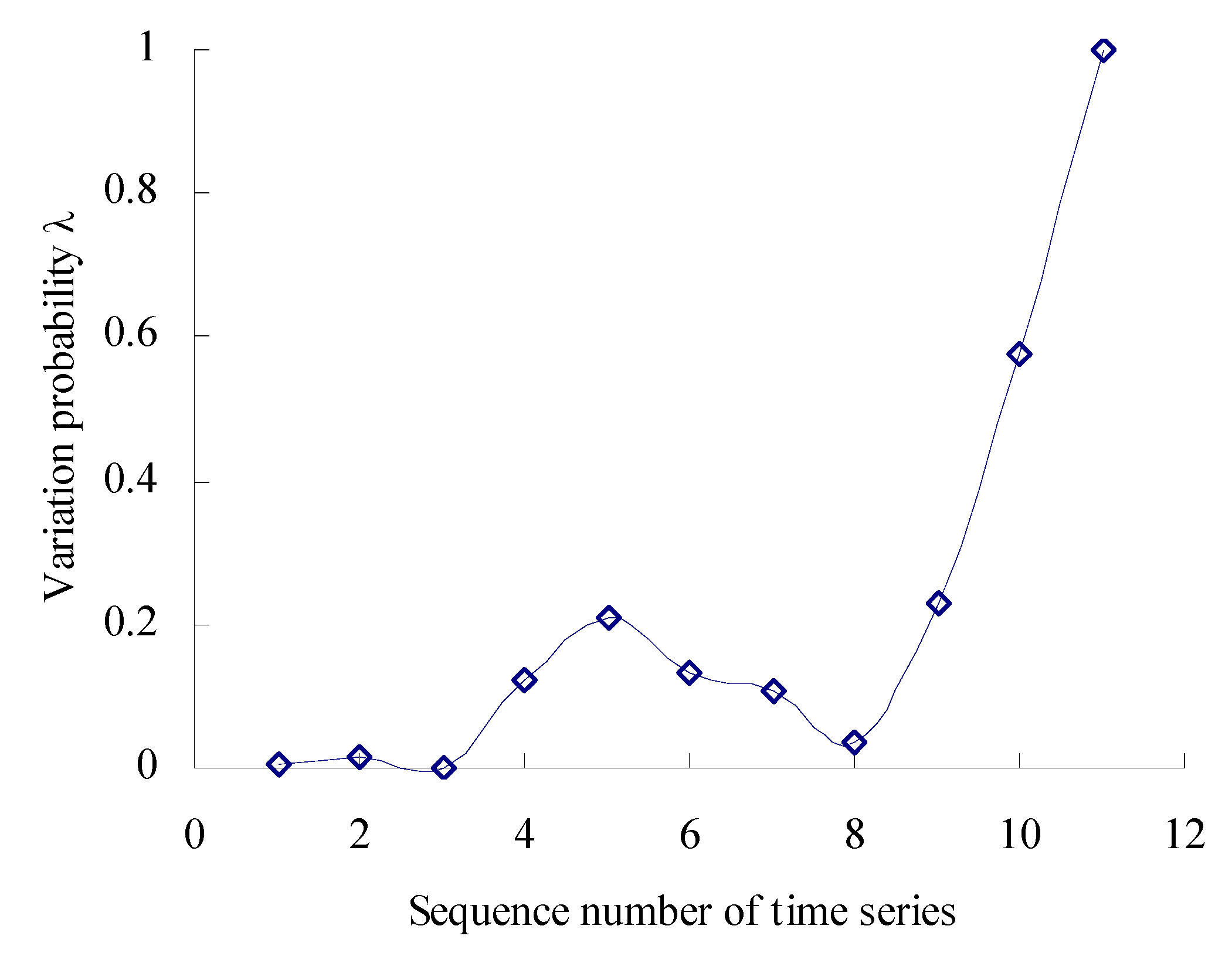
Based on the Equations (17) and (18), the numbers are calculated, respectively, that the 11 data samples fall outside the maximum entropy estimated interval [X_L1, X_U1] of intrinsic time series. According to the Poisson counting principle, the variation frequencies [λ₁, λ₂, λ₃, λ₄, λ₅, λ₆, λ₇, λ₈, λ₉, λ₁₀, λ₁₁] are as shown in Figure 5.

Figure 5. Variation probability curve.

As shown in Figure 5, the performance variation probability is non-linear and uncertain–relative to the intrinsic time series. Before the corresponding time interval of the third time series, the variation probability of the MTSB vibration performance is almost zero. Between the corresponding time interval of the third time series and the fifth time series, the variation probability has an increased trend. Between the corresponding time interval of the fifth time series and the eighth time series, the variation probability has a decreasing trend. Between the corresponding time interval of the eighth time series and the eleventh time series, the variation probability has a rapidly increasing trend.

3.1.2. Estimated Truth Value and Estimated Interval of Variation Probability of MTSB

The least-squares method is used to fit the variation probability with second-, third-, fourth-, fifth- and sixth-order polynomials. Based on the Equation (19), the fitting results are shown in Table 2 and Table 3, and Figure 6.

Table 2. Fitting using least-square method.

Order Number q of Polynomials	Expressions of Polynomials	Correlation Coefficient R2
Second order	G2(λn) = 0.0155λn2 − 0.1162λn + 0.2065	0.7863
Third order	G3(λn) = 0.0048λn3 − 0.0712λn2 + 0.3181λn − 0.3193	0.9390
Fourth order	G4(λn) = 0.0009λn4 − 0.0162λn3 + 0.0958λn2 − 0.1751λn + 0.0900	0.9725
Fifth order	G5(λn) = −0.0002λn5 + 0.0076λn4 − 0.0900λn3 + 0.4533λn2 − 0.9059λn + 0.5576	0.9860
Sixth order	G6(λn) = −0.00008λn6 + 0.0027λn5 − 0.0335λn4 + 0.1897λn3 − 0.4996λn2 + 0.5821λn − 0.2323	0.9955

Table 3. Fitting results of polynomials.

Sequence Number of Time Series	Variation Probability
	Third-Order Polynomial	Fourth-Order Polynomial	Fifth-Order Polynomial	Sixth-Order Polynomial
1	−0.0676	−0.00457	0.0224	0.0090
2	0.0707	0.0078	−0.0462	−0.0033
3	0.1243	0.0615	0.0524	0.0266
4	0.1222	0.1120	0.1477	0.1161
5	0.0933	0.1358	0.1712	0.1833
6	0.0665	0.1303	0.1293	0.1682
7	0.0706	0.1138	0.0764	0.0932
8	0.1346	0.1259	0.0879	0.0664
9	0.2873	0.2268	0.2331	0.2247
10	0.5577	0.4980	0.5486	0.6187
11	0.9746	1.0418	1.0108	1.0379

Figure 6. Variation probability curve fitting using least-square method.

The closer the correlation coefficient R² is to 1, the better the polynomial fitting. As shown in Table 4, the correlation coefficient R² for the second-order polynomial is less than 0.8. This shows that the fitting is worse than other higher-order polynomials. Therefore, the second-order polynomial is not used in further analysis.

Table 4. Estimated uncertainties U_λn of fitting effect using polynomials.

Sequence Number of Time Series n	Estimated Uncertainties Uλn	Sequence Number of Time Series n	Estimated Uncertainties Uλn
1	0.2010	7	0.1016
2	0.2361	8	0.1537
3	0.2088	9	0.1478
4	0.0878	10	0.2538
5	0.1935	11	0.1491
6	0.2194

Figure 6 shows that the fitted variation probability is almost identical with the actual variation probability for the fourth, tenth and eleventh time series. The fitting was performed using the least-square method by the third-order polynomial. With fittings using the least-square method by the fourth-order polynomial, the fitted variation probability values are basically identical with the actual values for the second, fourth, sixth, seventh and ninth time series. The fitted variation probability values are almost identical with the actual variation probability values for the third, sixth, ninth and eleventh time series when fitting was performed using the least-square method by the fifth-order polynomial. When fitting was performed using the least-square method by the sixth-order polynomial, the fitted variation probability values are basically identical with the actual values for the first, third, fourth, fifth, seventh, eighth and ninth time series. In short, the above four polynomials have their own advantages in fitting. Therefore, relevant information should be fully fused to effectively monitor the evolution process of rolling bearing vibration performance.

3.1.3. The Uncertainty of Variation Probability of MTSB

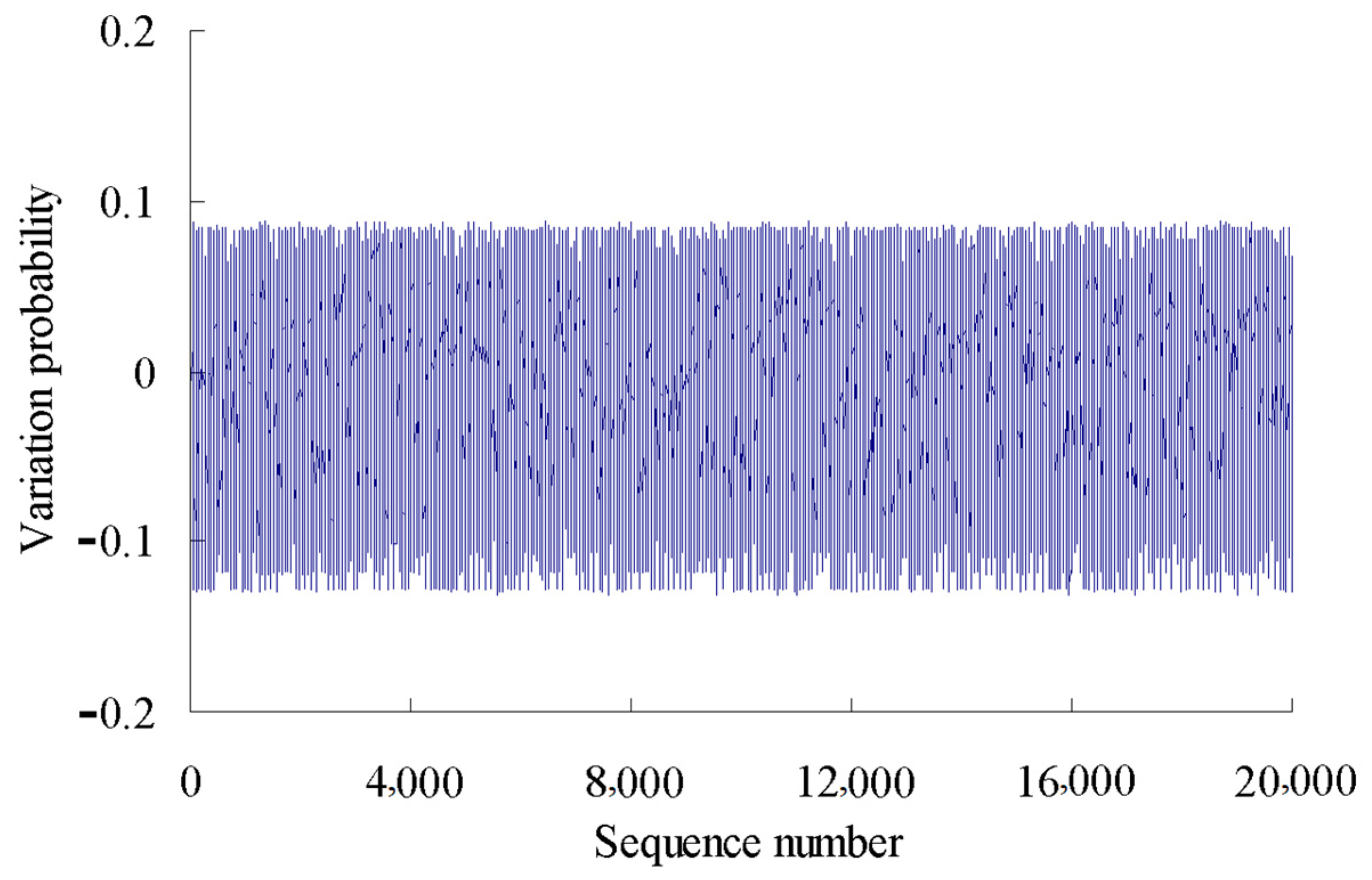
The variation probability of the first time series is taken as an example here. According to the grey bootstrap method, the number of bootstrap re-sampling is taken to be B = 20,000, and confidence level is taken to be P = 95%. Based on the Equations (20)–(32), the grey bootstrap sample Y_Bootstrap is obtained by sampling the sample data of fitting the variation probability values using the above four polynomials, as shown in Figure 7.

Figure 7. Sample data generated using grey bootstrap method.

Based on the maximum entropy method, the origin moments are obtained as [m₁₁, m₂₁, m₃₁, m₄₁, m₅₁] = [0.3813, 1.7553, 0.7854, 5.5473, 2.5368] for the grey bootstrap sample of variation probability. Lagrange multipliers are calculated as [c₀₁, c₁₁, c₂₁, c₃₁, c₄₁, c₅₁] = [1.3756, 0.8973, 0.3771, −0.3693, −0.0993, 0.0395] for the grey bootstrap sample of variation probability. Mapping parameter are gained as a₁ = 23.3049; b₁ = 0.5263.

The probability density function of the grey bootstrap sample Y_Bootstrap is shown in Figure 8.

Figure 8. Maximum entropy probability density function of grey bootstrap samples.

Assume that the confidence level α = 0.05 and the confidence level P = 95%. Based on the Equations (33)–(35), the estimated truth value and the estimated interval are obtained as λ₁₀ = 0.0057 and [λ_1L, λ_1U] = [−0.1299, 0.0711] for the grey bootstrap sample of variation probability of the first time series.

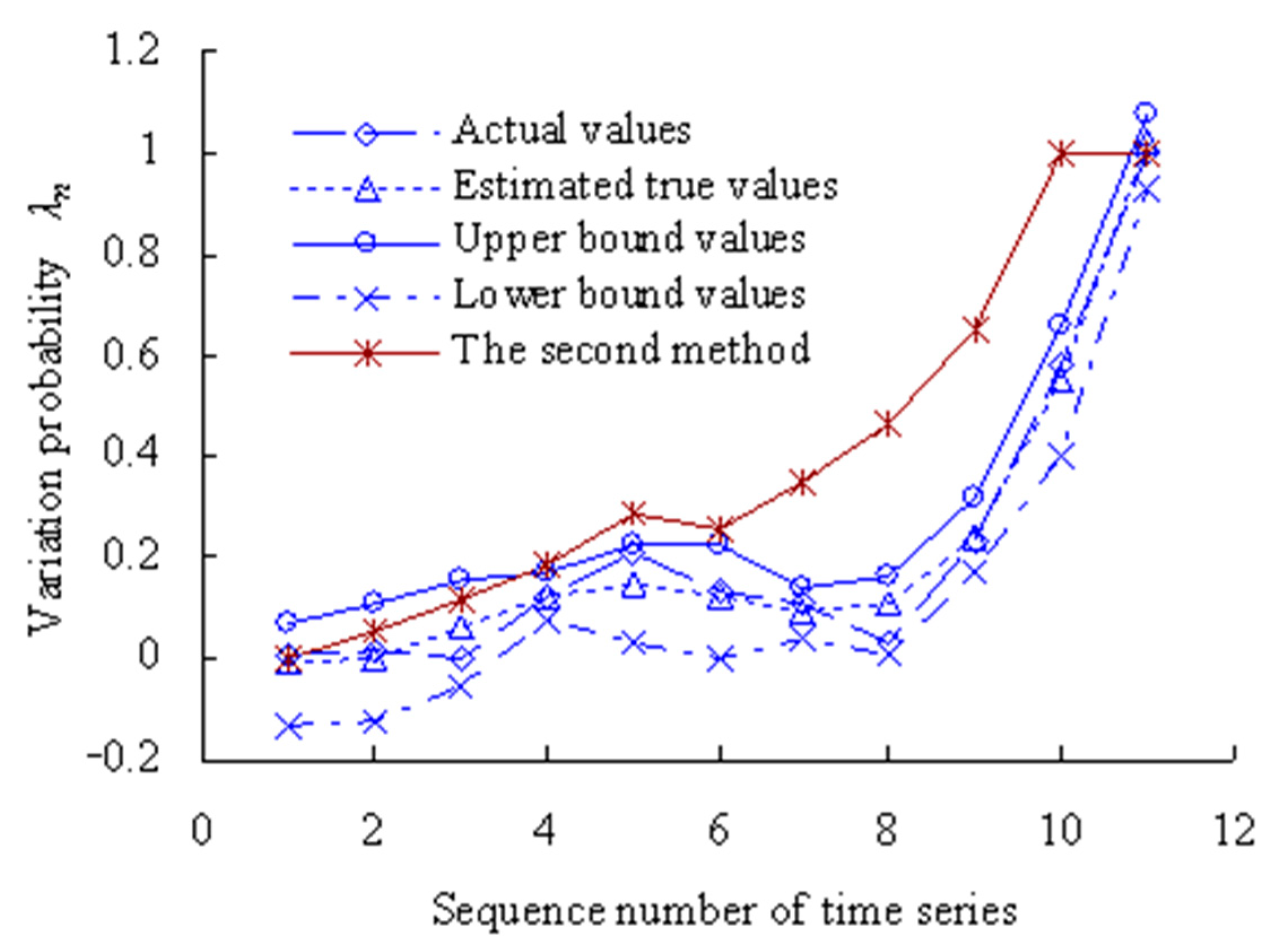
The grey bootstrap maximum entropy method is used to obtain the weighted average values, upper- and lower-bound values for the 11 time series under the condition that the confidence level is 0.05, as shown in Figure 9.

Figure 9. Estimated results of degradation probability of OVPS of MTSB.

Figure 9 shows that the values of variation probability calculated using the method in the Reference [34] (The second method) are larger than those calculated using this method. The variation probability has reached 1 for the 10th time series using the second method, which is less in line with the actual degradation process of OVPS of MTSB. Because the interference of random factors during the service process of MTSB was not taken into account.

Based on the Poisson counting process, the total number is calculated as η = 0 for variation probability sample data falling outside the upper-bound value λ_nU. That is, the reliability of the evaluation results is P_R = 100%, which satisfies P_R > P.

The estimated uncertainties are calculated for the variation probability of rolling bearing vibration performance, as shown in Table 4.

Based on the Equations (36)–(38), the dynamic average U_mean is calculated for the variation probability of time series as U_mean = 1.7515/11 = 0.1775.

3.1.4. PMR and PMRR of MTSB

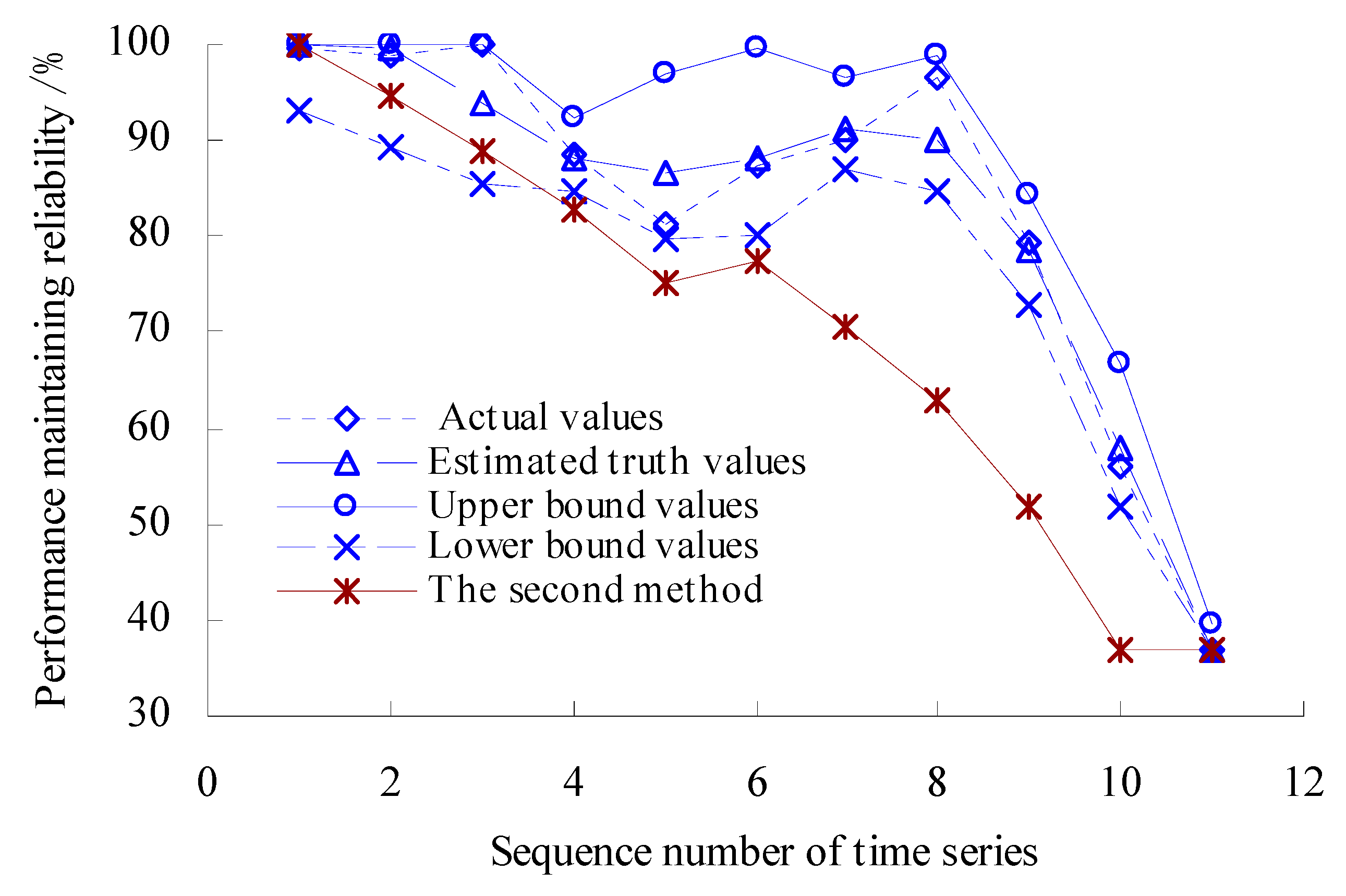
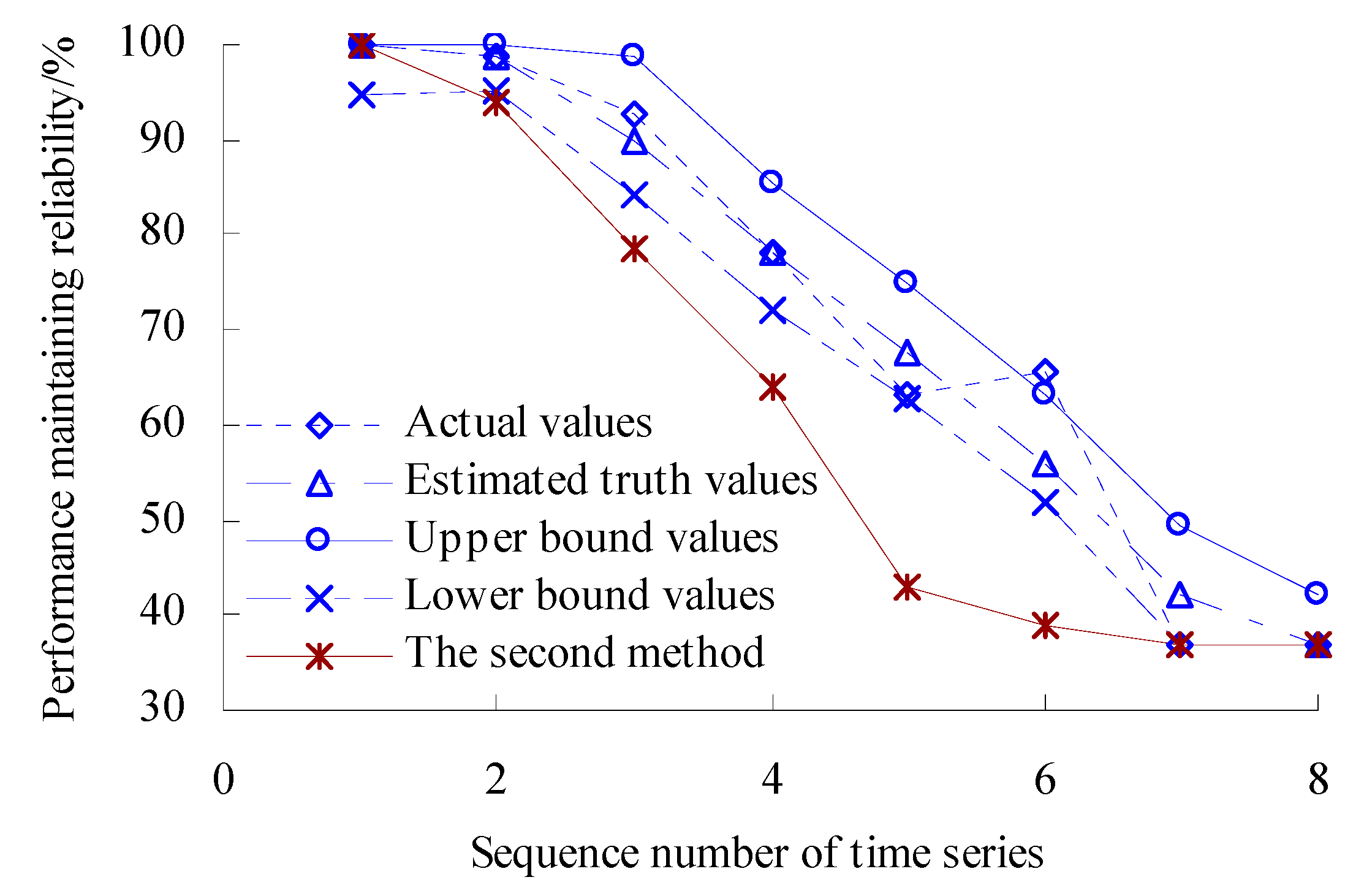
According to the calculated results of variation probability, the estimated true values R₀ and upper- and lower-bound intervals [R_L, R_U] are found as R₀ = exp(−λ_n0), R_L = exp(−λ_nU), R_U = exp(−λ_nL). The range of variation probability λ is [0, 1]. Here, 0 represents the OVPS of bearings without any variation, which is an ideal state with the reliability of bearing performance at 100%. On the other hand, 1 represents that the OVPS of spindle bearings fail completely and the performance is very unreliable. Therefore, if the value of λ_L is less than 0, let λ_L = 0 (artificially) in the process of solving the performance maintaining reliability. Based on the Equations (39)–(41), the dynamic evaluation results of the VPMR are shown in Figure 10.

Figure 10. Dynamic evaluation results of PMR.

As shown in Figure 10, the values of PMR remain unchanged before the time point corresponding to the third time series. During the period corresponding to the third time series to the fifth time series, the values of PMR have a decreasing trend. The value of PMR reaches the minimum, that is, 81.17442% for the fifth time series. The values of PMR have an increasing trend during the period corresponding to the fifth time series to the eighth time series. The values of PMR have a rapidly decreasing trend during the period corresponding to the eighth time series to the eleventh time series. Figure 10 shows that the values of PMR calculated using the second method are smaller than those calculated using this method.

The estimated true value curve coincides with the actual value curve for the PMR of spindle bearings, but the estimated true value curve is smoother. Moreover, the upper- and lower-bound curves envelope the actual value curves fully for the PMR, which verifies the rationality of the evaluation model again.

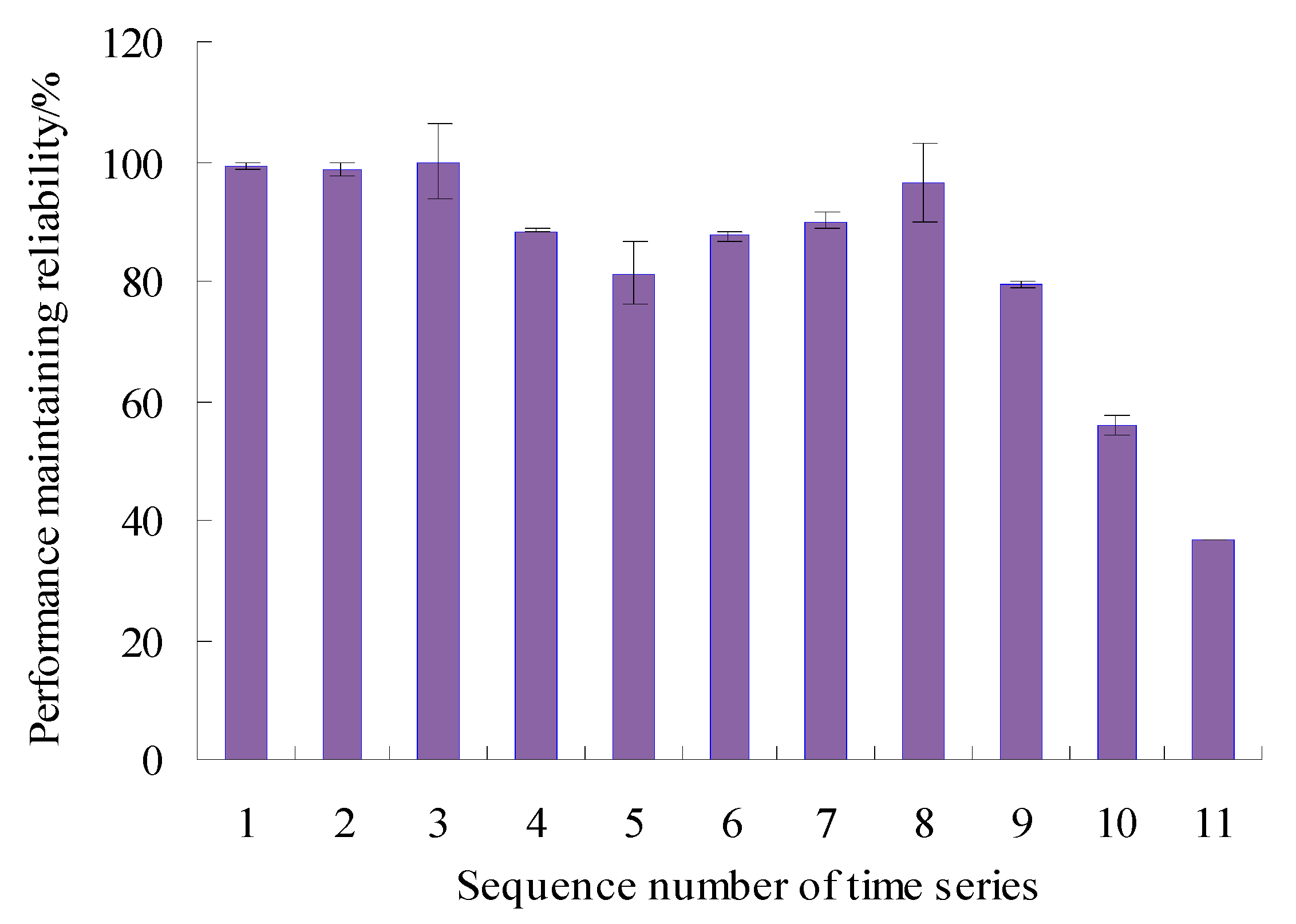
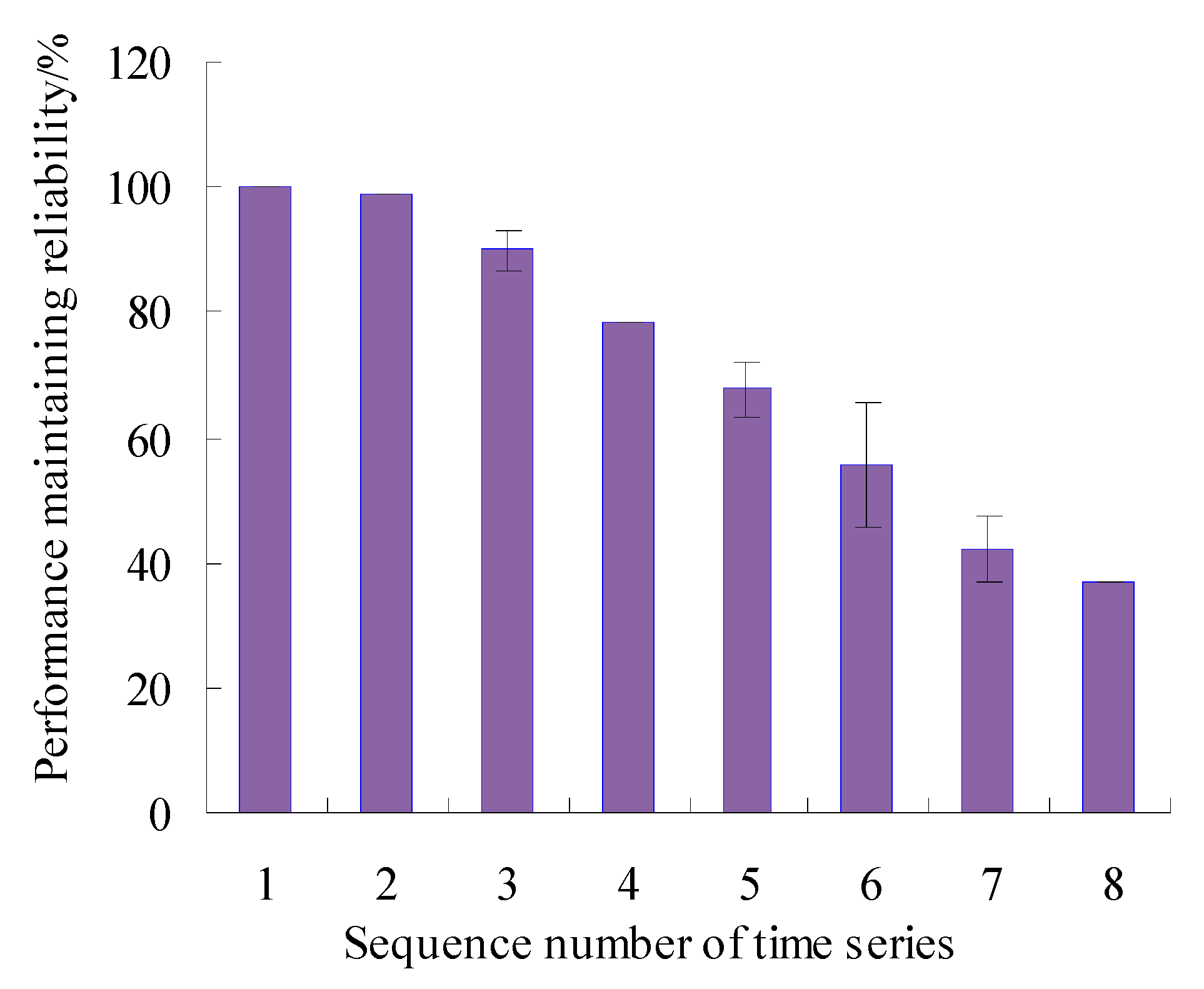
In order to visualize the difference between the estimated true value and the actual value of the PMR, the error bars of PMR are calculated, as shown in Figure 11.

Figure 11. Error bars of PMR.

As can be seen from Figure 11, the maximum error appears in the eighth time series, but is only 6.55%, and the errors were lower than 1.00% for the first, fourth, sixth, ninth, and tenth time series, which shows that the analysis results of the proposed method have good consistency. By analyzing the vibration data in Figure 3, it can be seen that the vibration performance has a sudden change or a large fluctuation during the period corresponding to these time series. Therefore, it is difficult to accurately estimate the values of PMR during the corresponding period.

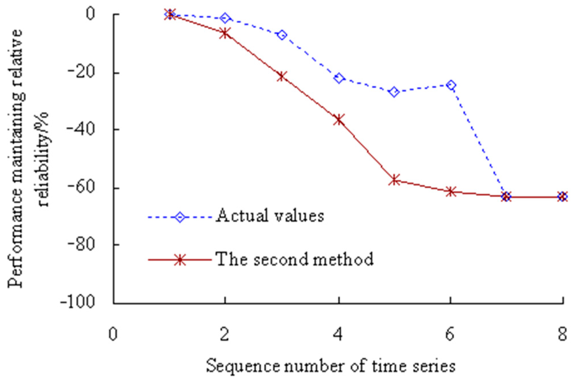
According to Equation (42), the dynamic evaluation results of the PMRR are shown in Figure 12.

Figure 12. Dynamic evaluation results of PMRR.

Figure 12 shows that the actual value of PMRR, d(λ₁), d(λ₃) ≥ 0%, which shows that the performance states of MTSB reaches the optimum and has almost no failure possibility at the corresponding stage; d(λ₂), d(λ₇), d(λ₈) ∈ [−15%, 0%), which shows that the performance states of MTSB is normal, and the degree failure of OVPS is very small; d(λ₄), d(λ₅), d(λ₆), d(λ₉) ∈ [−30%, −15%), which shows that the performance states of MTSB is gradually becoming worse, and the degree failure of OVPS is gradually increasing; d(λ₁₀), d(λ₁₁) < −30%, which shows that the performance states of MTSB is worse, and the degree failure of OVPS is very large. Thus, taking appropriate remedial measures are necessary steps before 6773 min, which can avoid serious safety accidents that are caused by the failure of OVPS.

Figure 12 also shows that the values of PMRR calculated using the second method are smaller than those calculated using this method. The values of PMRR, d(λ₇), d(λ₈), d(λ₉), d(λ₁₀), d(λ₁₁) < −30%, which shows that the degree failure of OVPS is very large after the corresponding time period of the 7th time series. However, this is less in line with the actual degradation process of OVPS of MTSB. Because the interference of random factors during the service process of MTSB was not taken into account.

3.2. Case 2

The test machine and the bearing used in this case are exactly the same as those of Case 1. The vibration data are shown in Figure 13 by changing the test conditions of the motor to a speed of 4000 r/min, an axial load of 4.17 kN, and a radial load of 4.58 kN.

Figure 13. Vibration signals of bearing performance (Case 2).

From the OVPS of the bearing, there are 5883 vibration signals. Among them, the 334th to 5933rd data points are divided into seven segments at 800 data intervals. The 5934th to 6216th data are separated into one segment, that is, the 8th segment.

3.2.1. Variation Probability of OVPS of MTSB (Case 2)

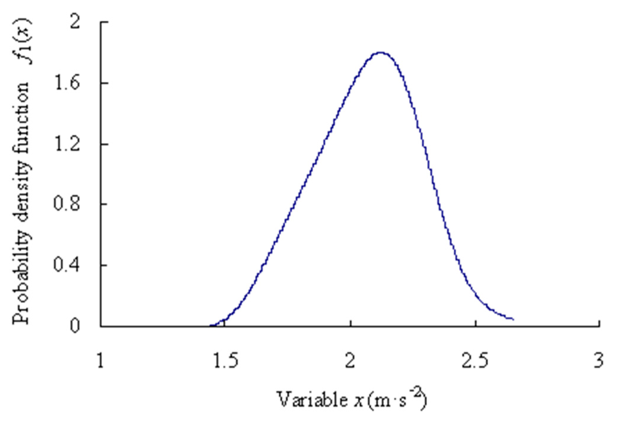
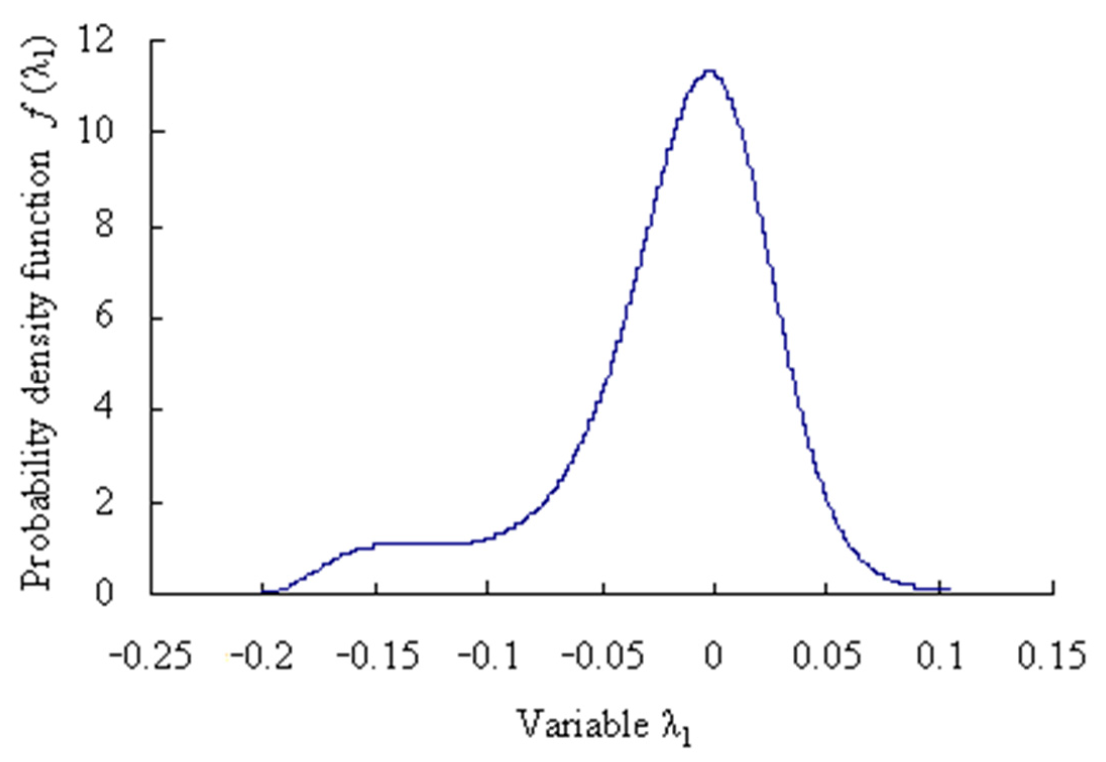
For the first time series, based on the Equations (1)–(12), the origin moments are obtained as [m₁₁, m₂₁, m₃₁, m₄₁, m₅₁] = [0.0768, 0.9388, 0.1046, 2.2771, 0.3843]. Lagrange multipliers are calculated as [c₀₁, c₁₁, c₂₁, c₃₁, c₄₁, c₅₁] = [0.5329, 0.3193, −0.3891, −0.1865, −0.0271, 0.0252]. Mapping parameter are gained as a₁ = 4.4481 and b₁ = −9.1186.

Assume that the significance level α is 0.05 and the confidence level is P = 95%, based on the Equations (13)–(16), the maximum entropy estimated interval of the intrinsic series is [1.5435, 2.5871] m·s⁻².

The probability density estimated truth function f₁(x) is calculated as shown in Figure 14.

Figure 14. Probability density function of data samples of intrinsic series (Case 2).

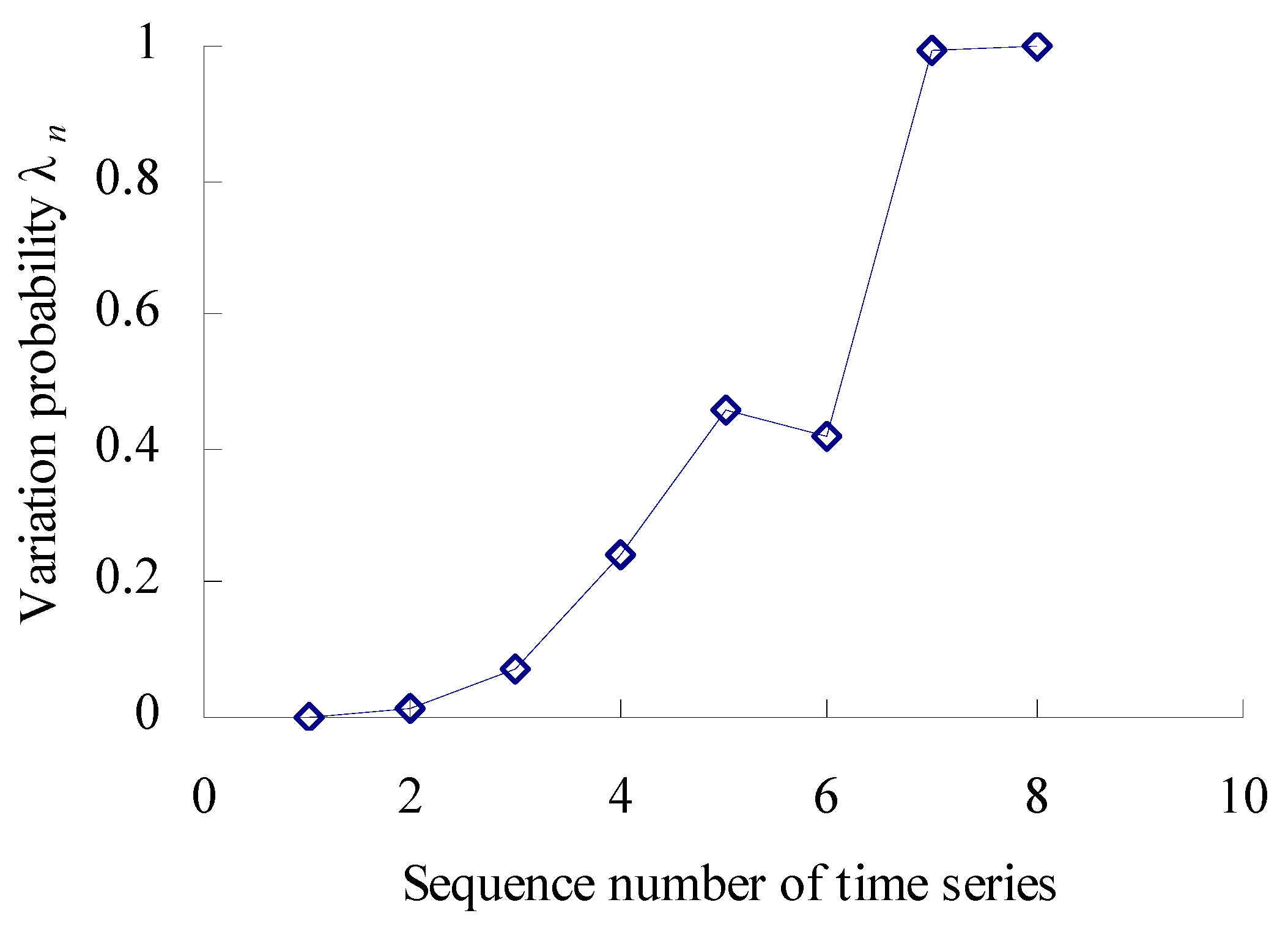
Based on the Equations (17) and (18), the numbers are calculated, respectively, that the 8 data samples fall outside the maximum entropy estimated interval of intrinsic time series. According to the Poisson counting principle, the variation frequencies [λ₁, λ₂, λ₃, λ₄, λ₅, λ₆, λ₇, λ₈, λ₉, λ₁₀, λ₁₁] = [0, 0.0136, 0.0738, 0.2450, 0.4563, 0.4370, 0.4213, 0.9963, 1], as shown in Figure 15.

Figure 15. Variation probability curve (Case 2).

As shown in Figure 15, the performance variation probability is non-linear and uncertain–relative to the intrinsic time series. Before the corresponding time interval of the second time series, the variation probability of the bearings’ vibration performance is almost zero. Between the corresponding time interval of the second time series and the fifth time series, the variation probability has an increased trend. Between the corresponding time interval of the fifth time series and the sixth time series, the variation probability has a decreasing trend. Between the corresponding time interval of the sixth time series and the seventh time series, the variation probability has a rapidly increasing trend.

3.2.2. Estimated Truth Value and Estimated Interval of Variation Probability of MTSB (Case 2)

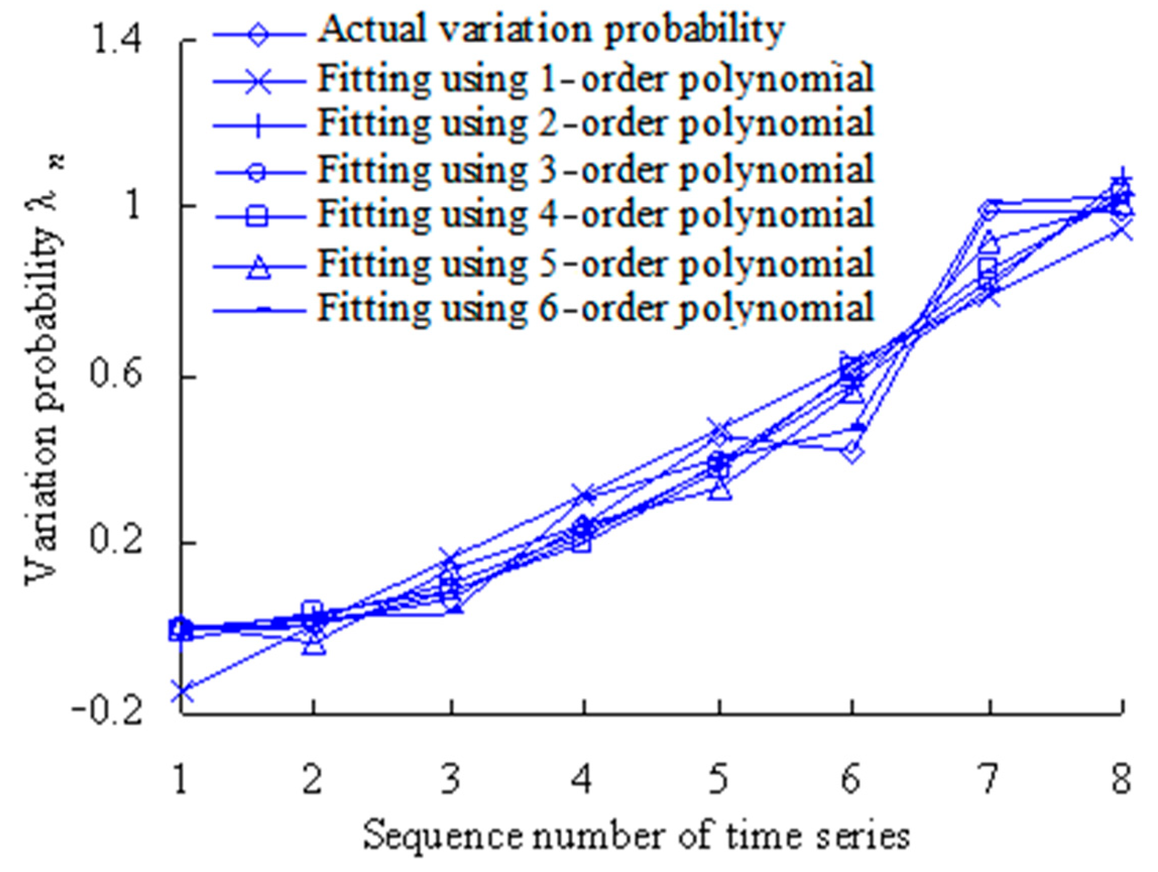
The least-squares method is used to fit the variation probability with first-, second-, third-, fourth-, fifth- and sixth-order polynomials. Based on the Equation (19), the fitting results are shown in Table 5 and Table 6, and Figure 16.

Table 5. Fitting using least-square method (Case 2).

Order Number q of Polynomials	Expressions of Polynomials	Correlation Coefficient R2
First order	G1(λn) = 0.1567λn − 0.3046	0.8905
Second order	G2(λn) = 0.0180λn2 − 0.0050λn − 0.0350	0.9373
Third order	G3(λn) = −0.0025λn3 + 0.0513λn2 − 0.1323λn + 0.0873	0.9404
Fourth order	G4(λn) = −0.0012λn4 + 0.0197λn3 − 0.0829λn2 + 0.1757λn − 0.1222	0.9428
Fifth order	G5(λn) = −0.0021λn5 + 0.0458λn4 − 0.3704λn3 + 1.3750λn2 − 2.1970λn + 1.1590	0.9596
Sixth order	G6(λn) = −0.0021λn6 + 0.0561λn5 − 0.5690λn4 + 2.8454λn3 − 7.2531λn2 + 8.8018λn − 3.8808	0.9910

Table 6. Fitting results of polynomials (Case 2).

Sequence Number n of Time Series	Variation Probability
	First-Order Polynomial	Second-Order Polynomial	Third-Order Polynomial	Fourth-Order Polynomial	Fifth-Order Polynomial	Sixth-Order Polynomial
1	−0.1479	−0.0220	0.0039	−0.0109	0.0103	−0.0017
2	0.0088	0.0269	0.0083	0.0359	−0.0324	0.0263
3	0.1655	0.1118	0.0857	0.0922	0.1433	0.0391
4	0.3222	0.2326	0.2213	0.2024	0.2475	0.3113
5	0.4789	0.3893	0.4003	0.3812	0.3365	0.4069
6	0.6356	0.5820	0.6078	0.6138	0.5626	0.4782
7	0.7923	0.8107	0.8290	0.8556	0.9230	1.0136
8	0.949	1.0752	1.0490	1.0325	1.0089	1.0357

Figure 16. Variation probability curve fitting using least-square method (Case 2).

The closer the correlation coefficient R² is to 1, the better the polynomial fitting. As shown in Table 5, the correlation coefficients R² for all polynomials are more than 0.8. Therefore, the first-order, second-order, third-order, fourth-order, fifth-order, and sixth-order polynomials will be used in further analysis.

Figure 16 shows that the fitted variation probability is almost identical with the actual variation probability for the second and fifth time series. The fitting was performed using the least-square method by the first-order polynomial. With fittings using the least-square method by the second-order polynomial, the fitted variation probability value is basically identical with the actual value for the fourth time series. The fitted variation probability values are almost identical with the actual variation probability values for the first, second and third time series when fitting was performed using the least-square method by the third-order polynomial. When fitting was performed using the least-square method by the fourth-order polynomial, the fitted variation probability value is basically identical with the actual value for the third time series. With fittings using the least-square method by the fifth-order polynomial, the fitted variation probability values are basically identical with the actual values for the fourth, seventh and eighth time series. The fitted variation probability values are almost identical with the actual variation probability values for the first, fifth, sixth, seventh and eighth time series when fitting was performed using the least-square method by the sixth-order polynomial. In short, the above six polynomials have their own advantages in fitting. Therefore, relevant information should be fully fused to effectively monitor the evolution process of rolling bearing vibration performance.

3.2.3. Uncertainty of Variation Probability of MTSB (Case 2)

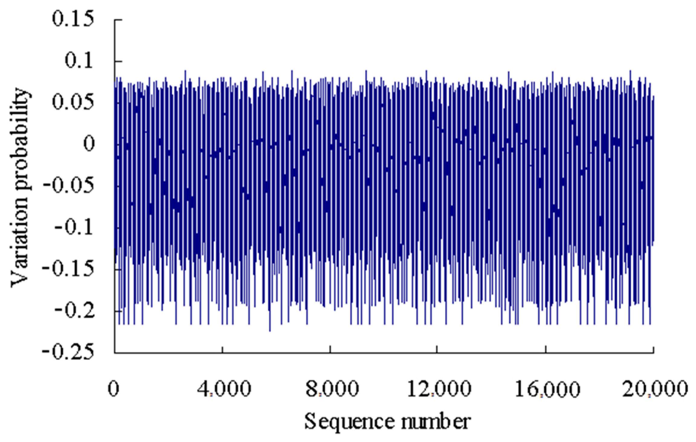
The variation probability of the first time series is taken as an example here. According to the grey bootstrap method, the number of bootstrap re-sampling is taken to be B = 20,000, and confidence level is taken to be P = 95%. Based on the Equations (20)–(32), the grey bootstrap sample Y_Bootstrap is obtained by sampling the sample data of fitting the variation probability values using the above six polynomials, as shown in Figure 17.

Figure 17. Sample data using grey bootstrap method (Case 2).

Based on the maximum entropy method, the origin moments are obtained as [m₁₁, m₂₁, m₃₁, m₄₁, m₅₁] = [0.7513, 1.1631, 1.2737, 2.3929, 3.1825] for the grey bootstrap sample of variation probability. Lagrange multipliers are calculated as [c₀₁, c₁₁, c₂₁, c₃₁, c₄₁, c₅₁] = [0.9174, 1.8886, 0.6202, −0.8485, −0.2844, 0.1335] for the grey bootstrap sample of variation probability. Mapping parameter are gained as a₁ = 15.7153; b₁ = 1.0616.

The probability density function of the grey bootstrap sample Y_Bootstrap is shown in Figure 18.

Figure 18. Maximum entropy probability density function of grey bootstrap samples (Case 2).

Assume that the confidence level α = 0.05 and the confidence level P = 95%. Based on the Equations (33)–(35), the estimated truth value and the estimated interval are obtained as λ₁₀ = −0.0197 and [λ_1L, λ_1U] = [−0.1534, 0.0536] for the grey bootstrap sample of variation probability of the first time series.

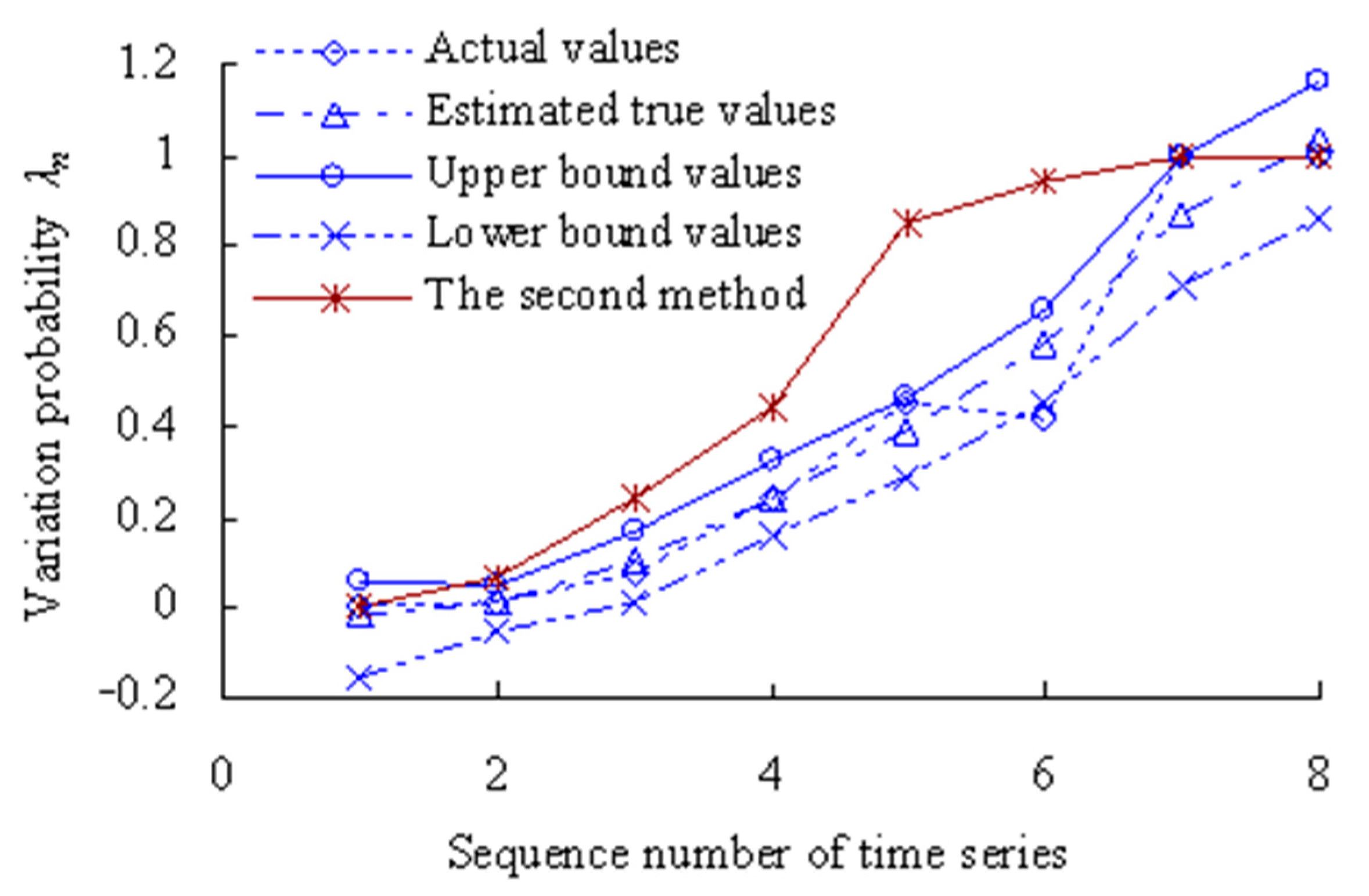
The grey bootstrap maximum entropy method is used to obtain the weighted average values, upper- and lower-bound values for the 8 time series under the condition that the confidence level is 0.05, as shown in Figure 19.

Figure 19. Estimated results of degradation probability of OVPS of MTSB (Case 2).

Figure 19 shows that the values of variation probability calculated using the method in the Reference [34] (The second method) are larger than those calculated using this method. The variation probability has reached 1 for the 7th time series using the second method, which is less in line with the actual degradation process of OVPS of MTSB. Because the interference of random factors during the service process of MTSB was not taken into account.

Based on the Poisson counting process, the total number is calculated as η = 0 for variation probability sample data falling outside the estimated upper-bound curve λ_nU. That is, the reliability of the evaluation results is P_R = 100%, which satisfies P_R > P.

The estimated uncertainty is calculated for the variation probability of rolling bearing vibration performance, as shown in Table 7.

Table 7. Estimated uncertainties U_λn of fitting effect using polynomials (Case 2).

Sequence Number n of Time Series	Estimated Uncertainties Uλn	Sequence Number n of Time Series	Estimated Uncertainties Uλn
1	0.2071	5	0.1751
2	0.1058	6	0.1950
3	0.1605	7	0.2890
4	0.1734	8	0.3041

Based on the Equations (36)–(38), the dynamic average U_mean is calculated for the variation probability of time series as U_mean = 1.4030/8 = 0.1169.

3.2.4. PMR and PMRR of MTSB (Case 2)

According to the calculated results of variation probability, the estimated true values R₀ and upper- and lower-bound intervals [R_L, R_U] are found as R₀ = exp(−λ_n0), R_L = exp(−λ_nU), R_U = exp(−λ_nL). The range of variation probability λ is [0, 1]. Here, 0 represents the OVPS of bearings without any variation, which is an ideal state with the reliability of bearing performance at 100%. On the other hand, 1 represents that the OVPS of spindle bearings fail completely and the performance is very unreliable. Therefore, if the value of λ_L is less than 0, let λ_L = 0 (artificially) in the process of solving the performance maintaining reliability. Based on the Equations (39)–(41), the dynamic evaluation results of the VPMR are shown in Figure 20.

Figure 20. Dynamic evaluation results of PMR (Case 2).

As shown in Figure 20, the values of VPMR remain unchanged before the time point corresponding to the second time series. During the period corresponding to the second time series to the fifth time series, the values of VPMR have a decreasing trend. The value of VPMR reaches the minimum, that is, 63.36544% for the fifth time series. The values of VPMR have an increasing trend during the period corresponding to the fifth time series to the sixth time series. The values of VPMR have a rapidly decreasing trend during the period corresponding to the sixth time series to the seventh time series. Figure 20 shows that the values of PMR calculated using the second method are smaller than those calculated using this method.

The estimated true value curve coincides with the actual value curve for the VPMR of spindle bearings, but the estimated true value curve is smoother. Moreover, the upper- and lower-bound curves envelope the actual value curves fully for the VPMR, which verifies the rationality of the evaluation model again.

In order to visualize the difference between the estimated true value and the actual value of the VPMR, the error bars of PMR are calculated, as shown in Figure 21.

Figure 21. Error bars of PMR (Case 2).

As can be seen from Figure 21, the maximum error appears in the sixth time series, but is only 9.91%, and the errors were lower than 0.05% for the first, second, fourth and eighth time series, which shows that the analysis results of the proposed method have good consistency. By analyzing the vibration data in Figure 13, it can be seen that the vibration performance has a sudden change or a large fluctuation during the period corresponding to these time series. Therefore, it is difficult to accurately estimate the values of VPMR during the corresponding period.

According to Equation (42), the dynamic evaluation results of the PMRR are shown in Figure 22.

Figure 22. Dynamic evaluation results of PMRR (Case 2).

Figure 22 shows that the actual value of PMRR, d(λ₁) ≥ 0%, which shows that the performance states of MTSB reaches the optimum and has almost no failure possibility at the corresponding stage; d(λ₂), d(λ₃) ∈ [−15%, 0%), which shows that the performance states of MTSB is normal, and the degree failure of OVPS is very small; d(λ₄), d(λ₅), d(λ₆) ∈ [−30%, −15%), which shows that the performance states of MTSB is gradually becoming worse, and the degree failure of OVPS is gradually increasing; d(λ₇), d(λ₈) < −30%, which shows that the performance states of MTSB is worse, and the degree failure of OVPS is very large. Thus, taking appropriate remedial measures are necessary steps before 5134 min, which can avoid serious safety accidents that are caused by the failure of OVPS.

Figure 22 also shows that the values of PMRR calculated using the second method are smaller than those calculated using this method. The values of PMRR, d(λ₄), d(λ₅), d(λ₆), d(λ₇), d(λ₈) < −30%, which shows that the degree failure of OVPS is very large after the corresponding time period of the 4th time series. However, this is less in line with the actual degradation process of OVPS of MTSB. Because the interference of random factors during the service process of machine tool spindle bearings (MTSB) was not taken into account.

In summary, the model realizes on-line monitoring of the degradation process of OVPS, which can give timely feedback so as to take preventive and remedial measures before the failure of OVPS for MTSB. Compared to the method in the Reference [8], the vibration threshold does not need to be set manually. Compared to other AI prediction methods, it does not require training on vibration signals, and the adjustment process of parameter is also omitted. In addition, there is no requirement for the length of time series. It is worth noting that, if there is an amount of missing data in the process of signal acquisition, the evaluation results of this approach may be inaccurate, and it cannot diagnose which component of bearings the fault occurred on.

4. Conclusions

By means of the Poisson process theory and taking variation probability as a time variable, the proposed model can effectively realize the dynamic evaluation for the degradation process of the OVPS for MTSB. This provides a technical and theoretical basis for on-line health detection and fault diagnosis of spindle bearings.

• The variation probability, obtained using the maximum entropy method and the Poisson counting principle, can accurately describe the degradation information and evolution process of the OVPS of MTSB.
• Considering the interference of random factors, the least-squares method by polynomial fitting, fused into the grey bootstrap maximum entropy method, can be used to calculate the dynamic mean uncertainty, so as to evaluate the random fluctuation state of OVPS.
• The results show the maximum relative errors between the estimated true value and the actual value of the PMR are 6.55% and 9.91% for the MTSB in the two studied cases: Case 1 and Case 2, respectively. Appropriate remedial measures should be taken before 6773min and 5134 min for the MTSB in the two studied cases: Case 1 and Case 2, respectively, which can avoid serious safety accidents caused by the failure of OVPS.

References

- Liu, J. A dynamic modelling method of a rotor-roller bearing-housing system with a localized fault including the additional excitation zone. J. Sound Vib. 2020, 469, 115144. [Google Scholar] [CrossRef]
- Zhang, W.H.; Deng, S.E.; Zhang, S.; Wang, J.; Zheng, J.T. Abnormal wear mechanism and improvement of high-speed cylindrical roller bearing. Shock Vib. 2021, 2021, 2522386. [Google Scholar] [CrossRef]
- Liu, J.; Xu, Y.; Pan, G. A combined acoustic and dynamic model of a defective ball bearing. J. Sound Vib. 2021, 501, 116029. [Google Scholar] [CrossRef]
- Nataraj, C.; Harsha, S.P. The effect of bearing cage run-out on the nonlinear dynamics of a rotating shaft. Commun. Nonlinear Sci. 2008, 13, 822–838. [Google Scholar] [CrossRef]
- Xia, X.T. Reliability analysis of zero-failure data with poor information. Qual. Reliab. Eng. Int. 2012, 28, 981–990. [Google Scholar] [CrossRef]
- Sinou, J.J. Non-linear dynamics and contacts of an unbalanced flexible rotor supported on ball bearings. Mech. Mach. Theory 2009, 44, 1713–1732. [Google Scholar] [CrossRef]
- Harris, T.A. Rolling Bearing Analysis, 3rd ed.; John Wiley & Sons, Inc.: New York, NY, USA, 1991. [Google Scholar]
- Ye, L.; Xia, X.T.; Chang, Z. Dynamic prediction for accuracy maintaining reliability of super-precision rolling bearing in service. Shock Vib. 2018, 2018, 7396293. [Google Scholar]
- Xia, X.T.; Meng, Y.Y.; Shi, B.J.; Qiu, M. Bootstrap forecasting method of uncertainty for rolling bearing vibration performance based on GM (1, 1). J. Grey Syst. 2015, 27, 78–92. [Google Scholar]
- Luo, Z.; Wang, Y.Q.; Zhou, W.H.; Wang, Z.Y. The grey relational approach for evaluating measurement uncertainty with poor information. Meas. Sci. Technol. 2015, 26, 125002. [Google Scholar] [CrossRef]
- Ye, L.; Hu, Y.S.; Deng, S.; Zhang, W.H.; Cui, Y.C.; Xu, J. A novel model for evaluating the operation performance status of rolling bearings based on hierarchical maximum entropy bayesian method. Lubricants 2022, 10, 97. [Google Scholar] [CrossRef]
- Huang, N.E.; Shen, Z.; Long, S.R. A new view of nonlinear water waves: The Hilbert spectrum. Annu. Rev. Fluid Mech. 1999, 31, 417–457. [Google Scholar] [CrossRef]
- Feldman, M. Time-varying vibration decomposition and analysis based on the Hilbert transform. J. Sound Vib. 2006, 295, 518–530. [Google Scholar] [CrossRef]
- Guo, W.; Tse, P.W. A novel signal compression method based on optimal ensemble empirical mode decomposition for bearing vibration signals. J. Sound Vib. 2013, 332, 423–441. [Google Scholar] [CrossRef]
- Zhou, S.H.; Qian, S.L.; Chang, W.B.; Xiao, Y.Y.; Cheng, Y. A novel bearing multi-fault diagnosis approach based on weighted permutation entropy and an improved SVM ensemble classifier. Sensors 2018, 18, 1934. [Google Scholar] [CrossRef] [PubMed]
- Zhou, J.B.; Xiao, M.H.; Niu, Y.; Ji, G.J. Rolling bearing fault diagnosis based on WGWOA-VMD-SVM. Sensors 2022, 22, 6281. [Google Scholar] [CrossRef]
- Fei, S.W. The hybrid method of VMD-PSR-SVD and improved binary PSO-KNN for fault diagnosis of bearing. Shock Vib. 2019, 2019, 4954920. [Google Scholar] [CrossRef]
- Pandya, D.H.; Upadhyay, S.H.; Harsha, S.P. Fault diagnosis of rolling element bearing by using multinomial logistic regression and wavelet packet transform. Soft Comput. 2014, 18, 255–266. [Google Scholar] [CrossRef]
- Lee, H.; Nguyen, N.T. Decision tree with optimal feature selection for bearing fault detection. J. Power Electron. 2008, 8, 101–107. [Google Scholar]
- Mian, T.; Choudhary, A.; Fatima, S. Vibration and infrared thermography based multiple fault diagnosis of bearing using deep learning. Nondestruct. Test. Eval. 2022, 38, 275–296. [Google Scholar] [CrossRef]
- Hoang, D.T.; Kang, H.J. A survey on deep learning based bearing fault diagnosis. Neurocomputing. 2019, 335, 327–335. [Google Scholar] [CrossRef]
- Zhang, B. Rolling bearing fault detection system and experiment based on deep learning. Comput. Intel. Neurosci. 2022, 2022, 8913859. [Google Scholar] [CrossRef] [PubMed]
- Tian, Y.L.; Liu, X.Y. A deep adaptive learning method for rolling bearing fault diagnosis using immunity. Tsinghua Sci. Technol. 2019, 24, 750–762. [Google Scholar] [CrossRef]
- Ruan, D.W.; Wang, J.; Yan, J.P.; Guhmann, C. CNN parameter design based on fault signal analysis and its application in bearing fault diagnosis. Adv. Eng. Inform. 2023, 55, 101877. [Google Scholar] [CrossRef]
- Sun, J.K.; Zhang, X.; Wang, J.X. Lightweight bidirectional long short-term memory based on automated model pruning with application to bearing remaining useful life prediction. Eng. Appl. Artif. Intel. 2023, 118, 105662. [Google Scholar] [CrossRef]
- Gu, K.; Zhang, Y.; Liu, X.B.; Li, H.; Ren, M.F. DWT-LSTM-Based fault diagnosis of rolling bearings with multi-sensors. Electronics 2021, 10, 2076. [Google Scholar] [CrossRef]
- Hao, S.J.; Ge, F.X.; Li, Y.M.; Jiang, J.Y. Multisensor bearing fault diagnosis based on one-dimensional convolutional long short-term memory networks. Measurement 2020, 159, 107802. [Google Scholar] [CrossRef]
- Xia, X.T.; Meng, Y.Y.; Qiu, M. Forecasting for variation process of reliability of rolling bearing vibration performance using grey bootstrap Poisson method. J. Mech. Eng. 2015, 51, 97–103. [Google Scholar] [CrossRef]
- Cong, F.Y.; Chen, J.; Pan, Y.N. Kolmogorov-Smirnov test for rolling bearing performance degradation assessment and prognosis. J. Vib. Control 2011, 17, 1337–1347. [Google Scholar] [CrossRef]
- Zhao, W.; Li, M.; Xiao, L. Nonlinear dynamic behaviors of a marine rotor-bearing system coupled with air bag and floating-raft. Shock Vib. 2015, 2015, 620968. [Google Scholar] [CrossRef]
- Chen, Y.S.; Yang, J.L.; Xu, Y.H.; Jiang, S.D.; Liu, X.D.; Wang, Q. Status self-validation of sensor arrays using gray forecasting model and bootstrap method. IEEE Trans. Instrum. Meas. 2016, 65, 1626–1640. [Google Scholar] [CrossRef]
- Bazilevs, Y.; Deng, X.; Korobenko, A.; Scalea, F.L.; Todd, M.D.; Taylor, S.G. Isogeometric fatigue damage prediction in large-scale composite structures driven by dynamic sensor data. J. Appl. Mech. T. ASME 2015, 82, 091008. [Google Scholar] [CrossRef]
- Rosunally, Y.Z.; Stoyanov, S.; Bailey, C.; Mason, P.; Campbell, S.; Monger, G.; Bell, I. Fusion approach for prognostics framework of heritage structure. IEEE Trans. Reliab. 2011, 60, 3–13. [Google Scholar] [CrossRef]
- Xia, X.T.; Zhu, W.H.; Liu, B. Reliability evaluation for the running state of the manufacturing system based on poor information. Math. Probl. Eng. 2016, 2016, 7627641. [Google Scholar] [CrossRef]
Disclaimer/Publisher’s Note: The statements, opinions and data contained in all publications are solely those of the individual author(s) and contributor(s) and not of MDPI and/or the editor(s). MDPI and/or the editor(s) disclaim responsibility for any injury to people or property resulting from any ideas, methods, instructions or products referred to in the content. |
© 2023 by the authors. Licensee MDPI, Basel, Switzerland. This article is an open access article distributed under the terms and conditions of the Creative Commons Attribution (CC BY) license (https://creativecommons.org/licenses/by/4.0/).