
Center of Mass Estimation Using a Force Platform and Inertial Sensors for Balance Evaluation in Quiet Standing


Abstract
1. Introduction
2. Estimation Methods
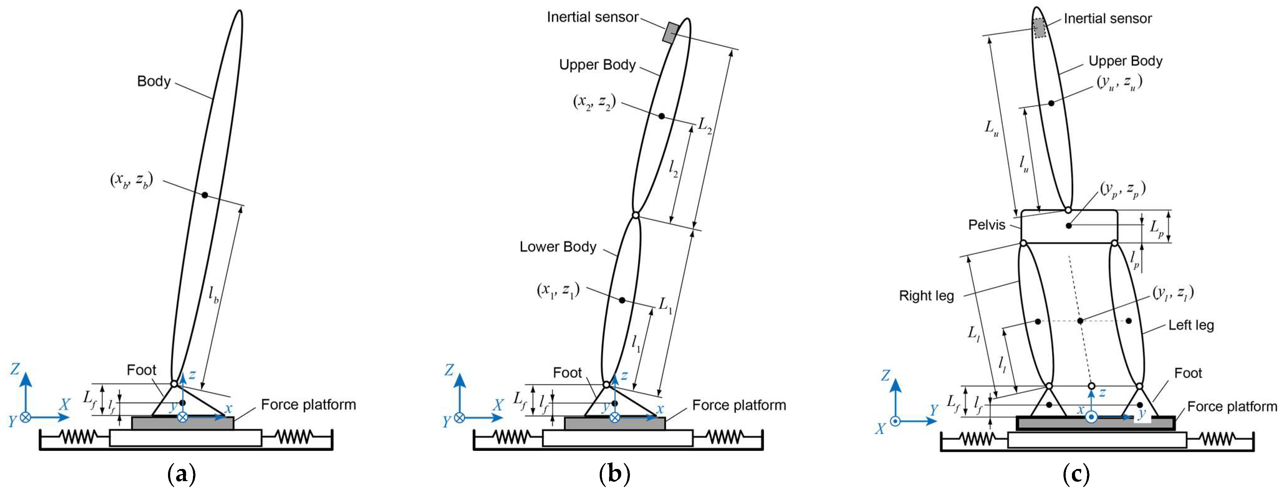
2.1. Modeling
2.2. COM Estimation Method
3. Verification Methods
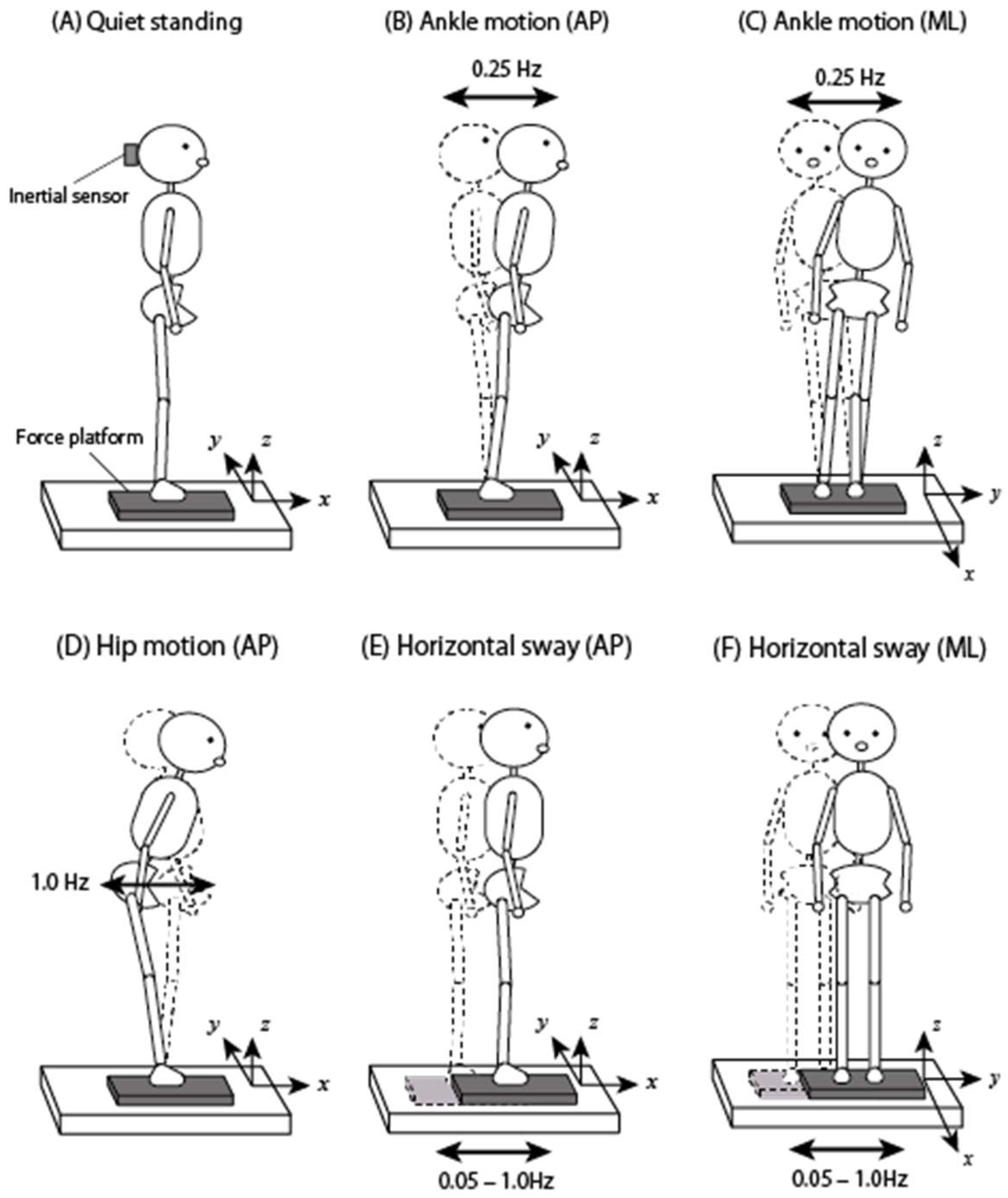
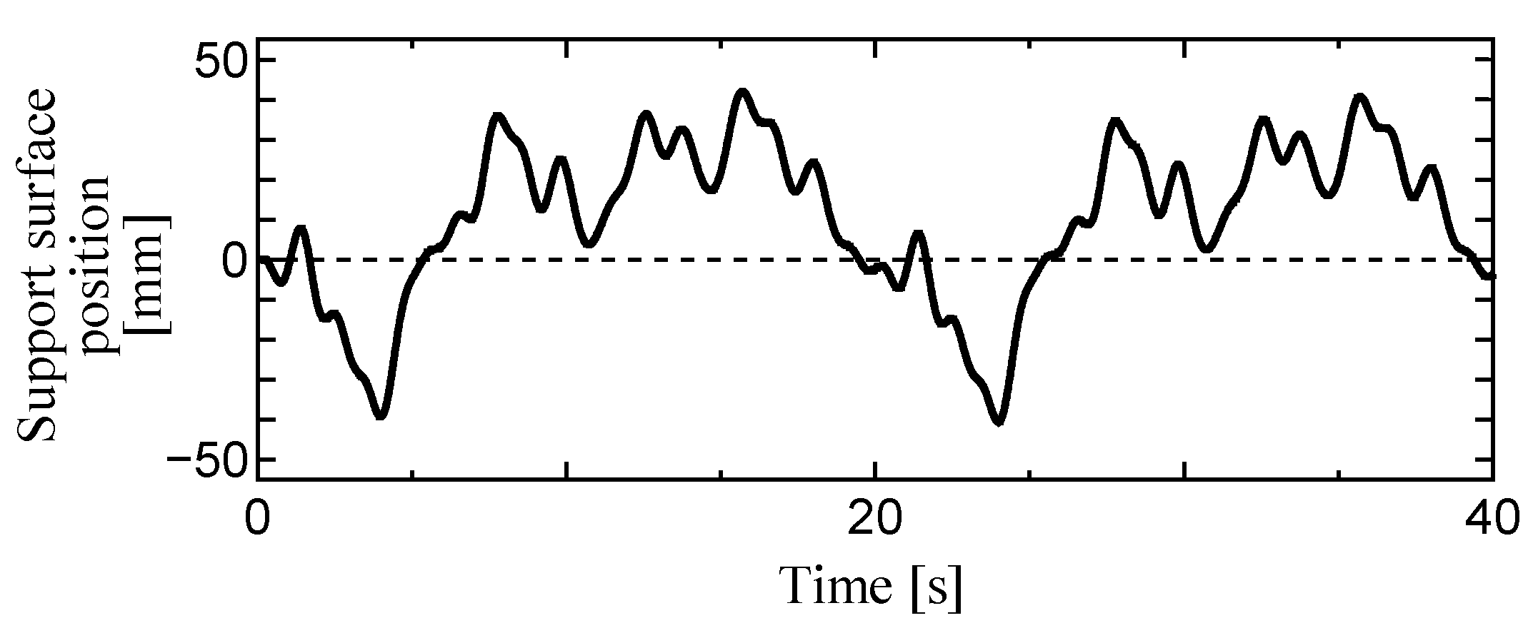
3.1. Experimental Protocol
3.2. Experimental Equipment
3.3. Post-Processing
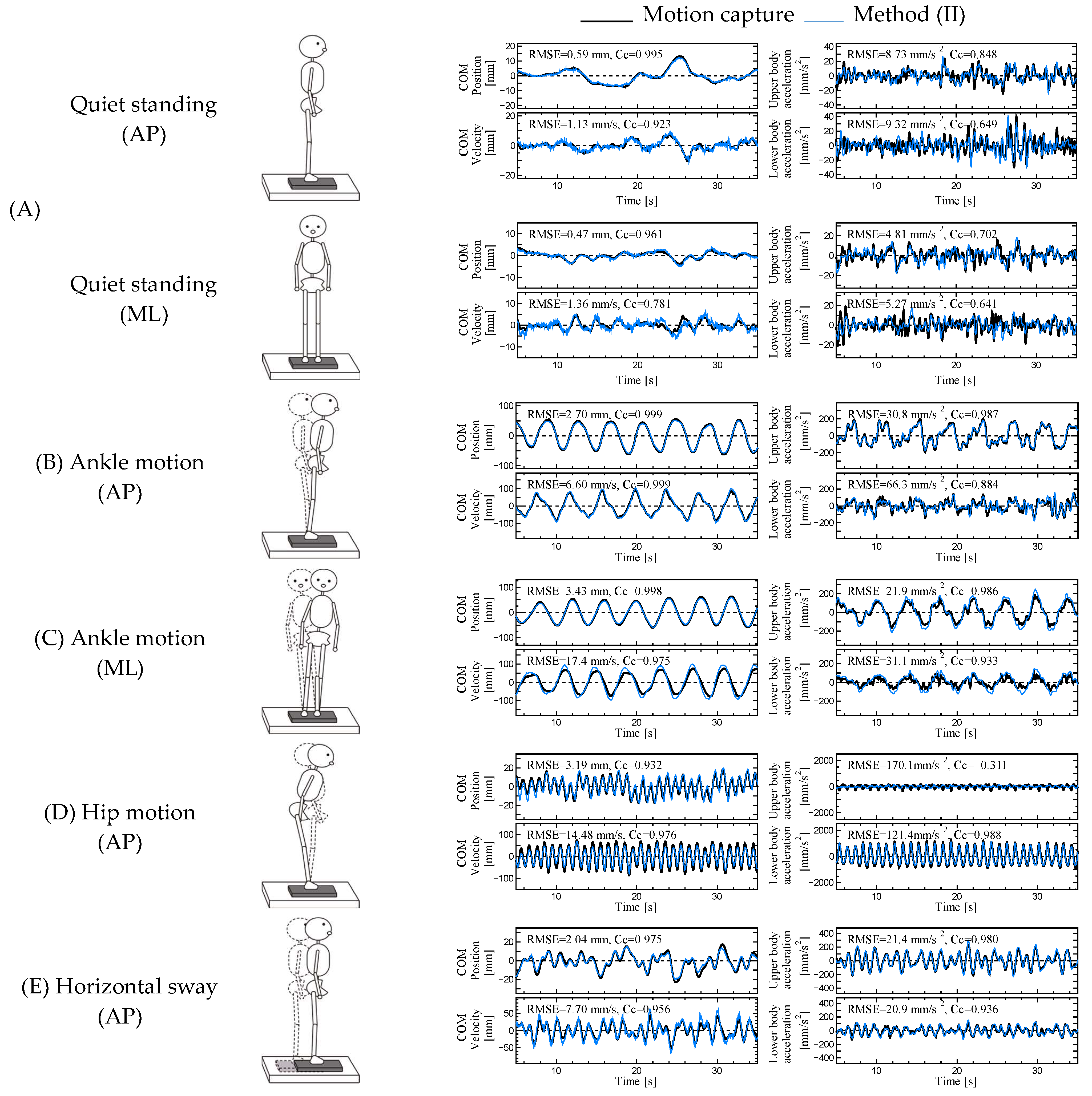
4. Results
5. Discussion
6. Conclusions
7. Patents
Author Contributions
Funding
Institutional Review Board Statement
Informed Consent Statement
Data Availability Statement
Conflicts of Interest
Appendix A
References
- Mansfield, A.; Danells, C.J.; Inness, E.; Mochizuki, G.; McIlroy, W.E. Between-limb synchronization for control of standing balance in individuals with stroke. Clin. Biomech. 2011, 26, 312–317. [Google Scholar] [CrossRef] [PubMed]
- Baratto, L.; Morasso, P.G.; Re, C.; Spada, G. A new look at posturographic analysis in the clinical context: Sway-density versus other parameterization techniques. Mot. Control 2002, 6, 246–270. [Google Scholar] [CrossRef] [PubMed]
- Kantner, R.M.; Rubin, A.M.; Armstrong, C.W.; Cummings, V. Stabilometry in balance assessment of dizzy and normal subjects. Am. J. Otolaryngol.-Head Neck Med. Surg. 1991, 12, 196–204. [Google Scholar] [CrossRef] [PubMed]
- Ludwig, O.; Kelm, J.; Hammes, A.; Schmitt, E.; Fröhlich, M. Neuromuscular performance of balance and posture control in childhood and adolescence. Heliyon 2020, 6, e04541. [Google Scholar] [CrossRef] [PubMed]
- Fino, P.C.; Mojdehi, A.R.; Adjerid, K.; Habibi, M.; Lockhart, T.E.; Ross, S.D. Comparing Postural Stability Entropy Analyses to Differentiate Fallers and Non-fallers. Ann. Biomed. Eng. 2016, 44, 1636–1645. [Google Scholar] [CrossRef]
- Zhou, J.; Habtemariam, D.; Iloputaife, I.; Lipsitz, L.A.; Manor, B. The Complexity of Standing Postural Sway Associates with Future Falls in Community-Dwelling Older Adults: The MOBILIZE Boston Study. Sci. Rep. 2017, 7, 2924. [Google Scholar] [CrossRef]
- Crétual, A. Which biomechanical models are currently used in standing posture analysis? Neurophysiol. Clin./Clin. Neurophysiol. 2015, 45, 285–295. [Google Scholar] [CrossRef]
- Błaszczyk, J.W. The use of force-plate posturography in the assessment of postural instability. Gait Posture 2016, 44, 1–6. [Google Scholar] [CrossRef]
- Chen, B.; Liu, P.; Xiao, F.; Liu, Z.; Wang, Y. Review of the upright balance assessment based on the force plate. International J. Environ. Res. Public Health 2021, 18, 2696. [Google Scholar] [CrossRef]
- Vette, A.H.; Sayenko, D.G.; Jones, M.; Abe, M.O.; Nakazawa, K.; Masani, K. Ankle muscle co-contractions during quiet standing are associated with decreased postural steadiness in the elderly. Gait Posture 2017, 55, 31–36. [Google Scholar] [CrossRef]
- Richmond, S.B.; Fling, B.W.; Lee, H.; Peterson, D.S. The assessment of center of mass and center of pressure during quiet stance: Current applications and future directions. J. Biomech. 2021, 123, 110485. [Google Scholar] [CrossRef] [PubMed]
- Winter, D.A. Human balance and posture control during standing and walking. Gait Posture 1995, 3, 193–214. [Google Scholar] [CrossRef]
- Yu, E.; Abe, M.; Masani, K.; Kawashima, N.; Eto, F.; Haga, N.; Nakazawa, K. Evaluation of Postural Control in Quiet Standing Using Center of Mass Acceleration: Comparison Among the Young, the Elderly, and People With Stroke. Arch. Phys. Med. Rehabil. 2008, 89, 1133–1139. [Google Scholar] [CrossRef]
- Oba, N.; Sasagawa, S.; Yamamoto, A.; Nakazawa, K. Difference in postural control during quiet standing between young children and adults: Assessment with center of mass acceleration. PLoS ONE 2015, 10, e0140235. [Google Scholar] [CrossRef] [PubMed]
- Ghai, S.; Nardone, A.; Schieppati, M. Human balance in response to continuous, predictable translations of the support base: Integration of sensory information, adaptation to perturbations, and the effect of age, neuropathy and Parkinson’s disease. Appl. Sci. 2019, 9, 5310. [Google Scholar] [CrossRef]
- Winberg, T.B.; Martel, D.R.; Hoshizaki, T.B.; Laing, A.C. Evaluation of amplitude- and frequency-based techniques for attenuating inertia-based movement artifact during surface translation perturbations. Gait Posture 2021, 86, 299–302. [Google Scholar] [CrossRef]
- van der Kooij, H.; van Asseldonk, E.; van der Helm, F.C.T. Comparison of different methods to identify and quantify balance control. J. Neurosci. Methods 2005, 145, 175–203. [Google Scholar] [CrossRef]
- Akçay, M.E.; Lippi, V.; Mergner, T. Visual Modulation of Human Responses to Support Surface Translation. Front. Hum. Neurosci. 2021, 15, 615200. [Google Scholar] [CrossRef]
- Nicolai, A.; Audiffren, J. Estimating Center of Mass Trajectory in Quiet Standing: A Review. In Proceedings of the Annual International Conference of the IEEE Engineering in Medicine and Biology Society, EMBS, Berlin, Germany, 23–27 July 2019; pp. 6854–6859. [Google Scholar]
- Zatsiorsky, V.M.; King, D.L. An algorithm for determining gravity line location from posturographic recordings. J. Biomech. 1997, 31, 161–164. [Google Scholar] [CrossRef]
- Caron, O.; Faure, B.; Brenière, Y. Estimating the centre of gravity of the body on the basis of the centre of pressure in standing posture. J. Biomech. 1997, 30, 1169–1171. [Google Scholar] [CrossRef]
- Gruben, K.G.; Boehm, W.L. Mechanical interaction of center of pressure and force direction in the upright human. J. Biomech. 2012, 45, 1661–1665. [Google Scholar] [CrossRef] [PubMed]
- Sopa, M.; Sypniewska-Kamińska, G.; Walczak, T.; Kamiński, H. Two-Dimensional Mechanical Model of Human Stability in External Force-Caused Fall. Appl. Sci. 2023, 13, 5068. [Google Scholar] [CrossRef]
- Gage, W.H.; Winter, D.A.; Frank, J.S.; Adkin, A.L. Kinematic and kinetic validity of the inverted pendulum model in quiet standing. Gait Posture 2004, 19, 124–132. [Google Scholar] [CrossRef] [PubMed]
- Fok, K.L.; Lee, J.; Vette, A.H.; Masani, K. Kinematic error magnitude in the single-mass inverted pendulum model of human standing posture. Gait Posture 2018, 63, 23–26. [Google Scholar] [CrossRef] [PubMed]
- King, D.L.; Zatsiorsky, V.M. Extracting gravity line displacement from stabilographic recordings. Gait Posture 1997, 6, 27–38. [Google Scholar] [CrossRef]
- Ae, M.; Tang, H.; Yokoi, T. Estimation of inertia properties of the body segments in Japanese athletes. Biomechanisum 1992, 11, 23–33. [Google Scholar] [CrossRef]
- Contini, R. Body segment parameters, Part II. Artif. Limbs 1972, 16, 1–19. [Google Scholar]
- Horak, F.B.; Nashner, L.M. Central programming of postural movements: Adaptation to altered support-surface configurations. J. Neurophysiol. 1986, 55, 1369–1381. [Google Scholar] [CrossRef]
- Sotirakis, H.; Patikas, D.A.; Papaxanthis, C.; Hatzitaki, V. Resilience of visually guided weight shifting to a proprioceptive perturbation depends on the complexity of the guidance stimulus. Gait Posture 2022, 95, 22–29. [Google Scholar] [CrossRef]
- Cofré Lizama, L.E.; Pijnappels, M.; Reeves, N.P.; Verschueren, S.M.; van Dieën, J.H. Centre of pressure or centre of mass feedback in mediolateral balance assessment. J. Biomech. 2015, 48, 539–543. [Google Scholar] [CrossRef]
- Kilby, M.C.; Slobounov, S.M.; Newell, K.M. Augmented feedback of COM and COP modulates the regulation of quiet human standing relative to the stability boundary. Gait Posture 2016, 47, 18–23. [Google Scholar] [CrossRef] [PubMed]
- Hirono, T.; Ikezoe, T.; Yamagata, M.; Kato, T.; Kimura, M.; Ichihashi, N. Relationship between postural sway on an unstable platform and ankle plantar flexor force steadiness in community-dwelling older women. Gait Posture 2021, 84, 227–231. [Google Scholar] [CrossRef] [PubMed]
- Komiya, M.; Maeda, N.; Narahara, T.; Suzuki, Y.; Fukui, K.; Tsutsumi, S.; Yoshimi, M.; Ishibashi, N.; Shirakawa, T.; Urabe, Y. Effect of 6-Week Balance Exercise by Real-Time Postural Feedback System on Walking Ability for Patients with Chronic Stroke: A Pilot Single-Blind Randomized Controlled Trial. Brain Sci. 2021, 11, 1493. [Google Scholar] [CrossRef] [PubMed]
- Lenzi, D.; Cappello, A.; Chiari, L. Influence of body segment parameters and modeling assumptions on the estimate of center of mass trajectory. J. Biomech. 2003, 36, 1335–1341. [Google Scholar] [CrossRef]
- Hof, A.L. Comparison of three methods to estimate the center of mass during balance assessment. J. Biomech. 2005, 38, 2134–2135. [Google Scholar] [CrossRef]
- Hof, A.L.; Gazendam, M.G.J.; Sinke, W.E. The condition for dynamic stability. J. Biomech. 2005, 38, 1–8. [Google Scholar] [CrossRef]


| Sagittal Plane | Frontal Plane | ||||
|---|---|---|---|---|---|
| Segment | Symbol | Value | Segment | Symbol | Value |
| Body | mb | 0.978 M | Legs | ml | 0.161 M |
| Jb | 0.0425 MH2 | Jl | 0.00524 MH2 | ||
| lb | 0.531 H | ll | 0.285 H | ||
| Lower body | m1 | 0.322 M | Ll | 0.460 H | |
| J1 | 0.00223 MH2 | Pelvis | mp | 0.187 M | |
| l1 | 0.285 H | lp | 0.056 H | ||
| L1 | 0.460 H | Lp | 0.144 H | ||
| Upper body | m2 | 0.656 M | Upper body | mu | 0.469 M |
| J2 | 0.0114 MH2 | Ju | 0.00714 MH2 | ||
| l2 | 0.191 H | lu | 0.109 H | ||
| L2 | 0.434 H | Lu | 0.290 H | ||
| Foot | Lf | 0.038 H | Foot | Lf | 0.038 H |
| Motion | Method | COM Position | COM Velocity | Lower Body Acceleration | Upper Body Acceleration |
|---|---|---|---|---|---|
| mm | mm/s | mm/s2 | mm/s2 | ||
| (A) Quiet Standing | RMS | 3.25 ± 1.09 | 2.36 ± 0.59 | 10.2 ± 4.2 | 11.0 ± 4.1 |
| (I) | 0.65 ± 0.21 | 1.83 ± 0.56 | - | - | |
| (II) | 0.59 ± 0.18 | 1.75 ± 0.55 | 9.6 ± 4.0 | 8.3 ± 4.1 | |
| (III) | 0.31 ± 0.12 | 0.72 ± 0.44 | - | - | |
| (IV) | 1.03 ± 0.67 | 3.71 ± 1.18 | - | - | |
| (B) Ankle Motion (AP) | RMS | 26.89 ± 7.70 | 33.70 ± 9.81 | 48.2 ± 13.0 | 85.6 ± 24.2 |
| (I) | 2.89 ± 1.45 | 9.73 ± 3.86 | - | - | |
| (II) | 2.62 ± 1.17 | 8.86 ± 3.77 | 33.7 ± 8.3 | 27.9 ± 8.9 | |
| (III) | 1.50 ± 0.43 | 2.29 ± 0.52 | - | - | |
| (IV) | 9.32 ± 6.96 | 10.81 ± 3.04 | - | - | |
| (D) Hip Motion (AP) | RMS | 9.03 ± 2.64 | 35.65 ± 14.50 | 421.5 ± 202.9 | 119.3 ± 66.5 |
| (I) | 15.10 ± 6.86 | 32.59 ± 15.28 | - | - | |
| (II) | 3.47 ± 1.67 | 12.16 ±5.36 | 100.0 ± 37.4 | 103.9 ± 57.7 | |
| (III) | 4.44 ± 2.06 | 24.01 ± 11.28 | - | - | |
| (IV) | 5.17 ± 3.34 | 10.22 ± 6.27 | - | - | |
| (E) Horizontal Sway (AP) | RMS | 10.89 ± 2.44 | 16.36 ± 1.76 | 50.3 ± 11.6 | 99.2 ± 11.3 |
| (I) | 1.99 ± 0.44 | 7.44 ± 0.81 | - | - | |
| (II) | 1.60 ± 0.34 | 6.90 ± 0.79 | 30.6 ± 8.4 | 32.2 ± 8.8 | |
| (III) | 1.21 ± 0.24 | 2.33 ± 0.50 | - | - | |
| (IV) | 12.15 ± 7.24 | 15.09 ± 3.92 | - | - |
| Motion | Method | COM Position | COM Velocity | Lower Body Acceleration | Upper Body Acceleration |
|---|---|---|---|---|---|
| mm | mm/s | mm/s2 | mm/s2 | ||
| (A) Quiet Standing | RMS | 1.51 ± 0.62 | 1.55 ± 0.53 | 9.4 ± 4.9 | 10.4 ± 6.1 |
| (I) | 0.56 ± 0.15 | 1.76 ± 0.46 | - | - | |
| (II) | 0.56 ± 0.15 | 1.75 ± 0.45 | 8.7 ±4.9 | 9.3 ± 6.3 | |
| (III) | 0.17 ± 0.07 | 0.66 ± 0.44 | - | - | |
| (IV) | 2.48 ± 2.78 | 5.23 ± 2.20 | - | - | |
| (C) Ankle Motion (ML) | RMS | 34.47 ± 8.77 | 42.86 ± 10.47 | 53.1 ±11.9 | 93.7 ± 21.4 |
| (I) | 3.60 ± 2.50 | 20.93 ± 5.38 | - | - | |
| (II) | 3.33 ± 1.96 | 19.67 ± 5.11 | 34.6 ±8.1 | 32.2 ± 8.4 | |
| (III) | 1.41 ± 0.80 | 2.16 ± 1.05 | - | - | |
| (IV) | 25.95 ± 22.62 | 33.36 ± 9.14 | - | - | |
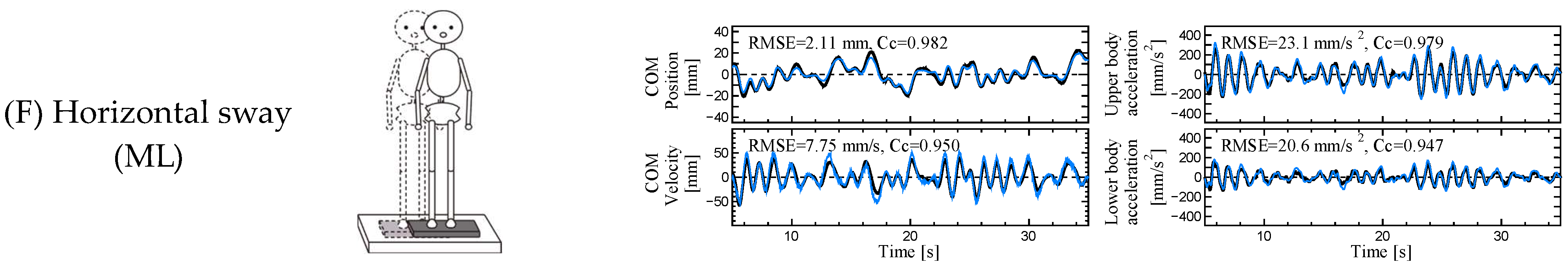
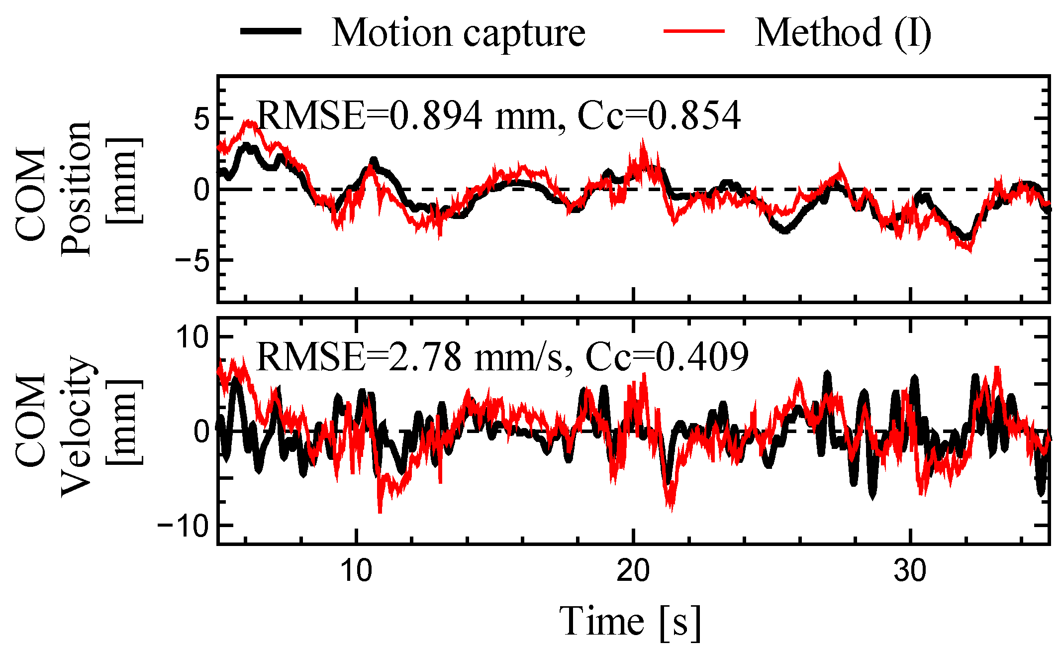
| (F) Horizontal Sway (ML) | RMS | 10.08 ± 1.98 | 19.10 ± 1.95 | 61.0 ±8.0 | 100.0 ± 11.9 |
| (I) | 2.32 ± 0.41 | 7.95 ± 1.16 | - | - | |
| (II) | 1.79 ± 0.36 | 7.38 ± 1.28 | 23.8 ±3.4 | 29.9 ± 5.8 | |
| (III) | 1.10 ± 0.24 | 1.91 ± 0.28 | - | - | |
| (IV) | 12.36 ± 7.71 | 16.39 ± 3.78 | - | - |
| Motion | Method | COM Position | COM Velocity | Lower Body Acceleration | Upper Body Acceleration |
|---|---|---|---|---|---|
| (A) Quiet Standing | (I) | 0.978 ± 0.023 | 0.778 ± 0.122 | - | - |
| (II) | 0.981 ± 0.020 | 0.781 ± 0.126 | 0.377 ± 0.136 | 0.446 ± 0.189 | |
| (III) | 0.997 ± 0.006 | 0.951 ± 0.073 | - | - | |
| (IV) | 0.954 ± 0.031 | 0.655 ± 0.152 | - | - | |
| (B) Ankle Motion (AP) | (I) | 0.998 ± 0.002 | 0.980 ± 0.024 | - | - |
| (II) | 0.998 ± 0.001 | 0.980 ± 0.025 | 0.689 ± 0.126 | 0.953 ± 0.031 | |
| (III) | 0.999 ± 0.001 | 0.999 ± 0.001 | - | - | |
| (IV) | 0.943 ± 0.060 | 0.970 ± 0.026 | - | - | |
| (D) Hip Motion (AP) | (I) | 0.102 ± 0.363 | 0.767 ± 0.071 | - | - |
| (II) | 0.938 ± 0.046 | 0.949 ± 0.043 | 0.958 ± 0.074 | 0.377 ± 0.429 | |
| (III) | 0.894 ± 0.063 | 0.893 ± 0.129 | - | - | |
| (IV) | 0.844 ± 0.183 | 0.942 ± 0.082 | - | - | |
| (E) Horizontal Sway (AP) | (I) | 0.984 ± 0.008 | 0.934 ± 0.013 | - | - |
| (II) | 0.989 ± 0.006 | 0.945 ± 0.011 | 0.813 ± 0.056 | 0.935 ± 0.028 | |
| (III) | 0.995 ± 0.002 | 0.992 ± 0.003 | - | - | |
| (IV) | 0.711 ± 0.196 | 0.840 ± 0.082 | - | - |
| Motion | Method | COM Position | COM Velocity | Lower Body Acceleration | Upper Body Acceleration |
|---|---|---|---|---|---|
| (A) Quiet Standing | (I) | 0.922 ± 0.062 | 0.636 ± 0.131 | - | - |
| (II) | 0.920 ± 0.068 | 0.623 ± 0.135 | 0.252 ± 0.125 | 0.339 ± 0.151 | |
| (III) | 0.991 ± 0.010 | 0.889 ± 0.100 | - | - | |
| (IV) | 0.713 ± 0.267 | 0.452 ± 0.159 | - | - | |
| (C) Ankle Motion (ML) | (I) | 0.998 ± 0.001 | 0.974 ± 0.017 | - | - |
| (II) | 0.998 ± 0.001 | 0.971 ± 0.019 | 0.872 ± 0.075 | 0.962 ± 0.034 | |
| (III) | 1.000 ± 0.000 | 0.999 ± 0.001 | - | - | |
| (IV) | 0.919 ± 0.120 | 0.975 ± 0.022 | - | - | |
| (E) Horizontal Sway (ML) | (I) | 0.974 ± 0.011 | 0.946 ± 0.019 | - | - |
| (II) | 0.985 ± 0.006 | 0.951 ± 0.022 | 0.924 ± 0.023 | 0.957 ± 0.022 | |
| (III) | 0.995 ± 0.002 | 0.996 ± 0.002 | - | - | |
| (IV) | 0.710 ± 0.195 | 0.873 ± 0.073 | - | - |
Disclaimer/Publisher’s Note: The statements, opinions and data contained in all publications are solely those of the individual author(s) and contributor(s) and not of MDPI and/or the editor(s). MDPI and/or the editor(s) disclaim responsibility for any injury to people or property resulting from any ideas, methods, instructions or products referred to in the content. |
© 2023 by the authors. Licensee MDPI, Basel, Switzerland. This article is an open access article distributed under the terms and conditions of the Creative Commons Attribution (CC BY) license (https://creativecommons.org/licenses/by/4.0/).
Share and Cite
Sonobe, M.; Inoue, Y. Center of Mass Estimation Using a Force Platform and Inertial Sensors for Balance Evaluation in Quiet Standing. Sensors 2023, 23, 4933. https://doi.org/10.3390/s23104933
Sonobe M, Inoue Y. Center of Mass Estimation Using a Force Platform and Inertial Sensors for Balance Evaluation in Quiet Standing. Sensors. 2023; 23(10):4933. https://doi.org/10.3390/s23104933
Chicago/Turabian StyleSonobe, Motomichi, and Yoshio Inoue. 2023. "Center of Mass Estimation Using a Force Platform and Inertial Sensors for Balance Evaluation in Quiet Standing" Sensors 23, no. 10: 4933. https://doi.org/10.3390/s23104933
APA StyleSonobe, M., & Inoue, Y. (2023). Center of Mass Estimation Using a Force Platform and Inertial Sensors for Balance Evaluation in Quiet Standing. Sensors, 23(10), 4933. https://doi.org/10.3390/s23104933