Article

Formation Control of Automated Guided Vehicles in the Presence of Packet Loss

School of Computer Science and Information Technology, University College Cork, T12 K8AF Cork, Ireland
*
Author to whom correspondence should be addressed.
Sensors 2022, 22(9), 3552; https://doi.org/10.3390/s22093552
Submission received: 30 March 2022 / Revised: 27 April 2022 / Accepted: 28 April 2022 / Published: 7 May 2022

Abstract

:
This paper presents the formation tracking problem for non-holonomic automated guided vehicles. Specifically, we focus on a decentralized leader–follower approach using linear quadratic regulator control. We study the impact of communication packet loss—containing the position of the leader—on the performance of the presented formation control scheme. The simulation results indicate that packet loss degrades the formation control performance. In order to improve the control performance under packet loss, we propose the use of a long short-term memory neural network to predict the position of the leader by the followers in the event of packet loss. The proposed scheme is compared with two other prediction methods, namely, memory consensus protocol and gated recurrent unit. The simulation results demonstrate the efficiency of the long short-term memory in packet loss compensation in comparison with memory consensus protocol and gated recurrent unit.

1. Introduction

Automated guided vehicles (AGVs) along with their formation control are a key technology for Industry 4.0 as they automate the coordinated movement of materials and components in manufacturing environments in a safe, secure, and operationally efficient manner [1,2]. In many applications, formation control refers to the process by which a group of autonomous vehicles follows a predefined trajectory while maintaining a desired spatial pattern [3]. Multi-agent formation control systems have received considerable attention in the research literature due to the inherent difficulties associated with the control and coordination strategies, especially in the absence of a central controller. AGV formation control has been extensively used in smart factories and warehouse environments in a mobile robot-based production line system [4]. Formation control has a wide range of applications, including vehicle platoon control [5], cooperative transportation of large or heavy loads carried by multiple mobile robots, or automated guided vehicles (AGVs) [6]. Formation control [7] addresses various sub-problems such as localization [8], obstacle avoidance [9], and distributed path planning [10], with numerous studies on these topics. Due to its simplicity and scalability, the leader–follower approach is a widely adopted formation control method [11]. This method selects one or more robots as leaders to guide and move along the desired trajectory, while the remaining robots are selected as followers to track the leader(s) paths. A leader–follower formation control problem can be considered a tracking problem in control systems, where the leader moves along the desired trajectory, and the followers track the leader, maintaining the required formation [3]. We consider that each robot’s (e.g., leader, follower) control procedure only uses local measurements and is not based on a centralized controller. Consensus control is another type of formation control in which all robots coordinate and make decisions based on information from their neighbours to achieve consensus [12].
Generally, the AGVs/robots exchange formation control information through a wireless network [10], which plays a vital role in interconnecting the AGVs. Formation control is vulnerable to wireless network uncertainties such as wireless channel noise, communication delay, and communication packet losses. These uncertainties can result in a variety of complex dynamic behaviours in control systems, such as divergence, oscillation, and instability [13]. Most existing studies assume ideal communication links and do not consider the effect of packet loss or delay [14,15,16]. There are only a few works that consider communication delay, while the packet loss is generally ignored [12,17,18,19,20,21].
However, packet loss in the communication network has a significant impact on the performance of any industrial process control system [22], specifically the trajectory tracking performance of a robotic formation. In the formation control of robots, holonomic and non-holonomic robots are two types of robots which are widely used in industry; while holonomic robots move regardless of their heading angle/orientation, non-holonomic robots such as differential drive robots are unable to move into arbitrary directions due to a non-holonomic constraint. As a result, they require sophisticated control mechanisms, and the impact of packet loss on the formation control of non-holonomic differential drive robots is significant. Holonomic robot formation is more resilient to network uncertainties than non-holonomic robot formation [23]. To mitigate the effects of packet loss, communication networks typically use re-transmissions to ensure that the data are received at the intended receiver. However, re-transmission will increase the transmission delay [18]. On the other hand, a range of control approaches such as robust control [24], model predictive control [25], sliding mode control [13], and various estimators [26] or filters [27] are widely used to address packet loss from a control perspective.
Machine learning can also be a useful tool to mitigate packet loss, and its efficiency has been demonstrated in a variety of wireless network applications within the Internet of Things context, including network management, congestion avoidance, and resource allocation optimization [28]. As a result, various studies have been conducted on the predictive capabilities of machine learning, particularly deep learning approaches such as long short-term memory (LSTM) [29]. To the best of our knowledge, no prior research has used deep learning techniques to address the effect of packet loss on formation control. Inspired by the above discussions, we propose using LSTM to control the formation of non-holonomic differential drive AGVs in the presence of packet loss. LSTM is a powerful technique for forecasting time series and classifying data [30]. The LSTM algorithm is capable of extracting features from time series over a longer time span and of solving the vanishing gradient problem [31]. In this study, the leader follows a trajectory, which is a sequence of locations over time. Thus, LSTM is proposed to forecast the leader’s position, and followers use this predicted value as needed (whenever the position data sent by the leader is lost by the wireless network). As the quality of the wireless communication deteriorates, followers frequently predict the leader’s position using LSTM for tracking the leader’s trajectory. Our results show that LSTM outperforms gated recurrent units (GRUs) and memory consensus protocol (MCP). MCP is a well-known technique that stores each neighbour’s previously received data and uses them when a packet is not received by a neighbour [32]. MCP becomes inefficient as the number of consecutive packet losses increases [33]. The GRU architecture is similar to the LSTM, but it lacks an output gate, which reduces the calculation burden and simplifies implementation [34]. However, LSTM prediction usually outperforms GRU prediction [35]. We model the packet loss using a Bernoulli distribution and evaluate LSTM predictions with a packet loss of 30 and 50 percent.
The following are the major contributions of this paper:
  • Study of decentralized leader–follower formation control for non-holonomic automated guided vehicles using linear quadratic regulator (LQR). LQR is a simple yet popular control approach that can be easily implemented and that has not yet been used for formation control.
  • Analysis of the impact of packet loss on the formation control of AGVs.
  • Improving the performance of a linear quadratic regulator (LQR) controller via machine learning, e.g., LSTM, to deal with packet losses, rather than using a highly non-linear and complicated controller such as a sliding mode controller.
  • Development of a mechanism to compensate for packet loss with LSTM and the application of the mechanism to the formation control of non-holonomic differential drive robots, which are more sensitive to network uncertainties due to non-holonomic constraints.
  • Comparing LSTM with GRU and MCP for the compensation of 30 and 50 percent packet loss through simulation in MATLAB/SIMULINK.
The rest of this paper is organized as follows. In Section 2, related work focused on the compensation of packet loss for AGVs is presented. Section 3 discusses how to model differential drive robots mathematically. A controller is designed in Section 4. In Section 5.1, the vulnerability of the system to packet loss is demonstrated. In Section 5.2, an LSTM network is used to counteract the negative impact of packet loss. Prediction accuracy of LSTM, GRU, and MCP are compared in Section 6.1. Simulations are used to evaluate the proposed method’s performance in Section 6.2. Finally, the conclusion and suggestions for future work are presented in Section 7.

2. Related Work

In this section, we mainly discuss prior research that has developed algorithms and controllers to deal with packet loss in the formation control of AGVs. The authors in [36] concluded that by reducing the number of control updates and transmissions, the wireless communication channel is less congested and hence packet losses can be minimized. However, the authors did not propose any mechanisms to address the effect of packet loss, which can affect the performance of their formation control.
In [33], a networked predictive controller and two algorithms are developed to cope with consecutive packet loss and communication delay for non-linear wheeled mobile robots. The authors simulated the effect of packet loss by considering a tunnel the robot travels through that is no longer detectable with cameras and associated servers [33]. A well-quantified analysis of packet loss and its effects is missing.
A consensus-based tracking control strategy was studied for leader–follower formation control of multiple mobile robots under packet loss [37]. A novel multiple Lyapunov functional candidate and linear matrix inequality (LMIs) ensure that the robots reach consensus when packet loss and communication weight (representing the rate of information flow between agents) are taken into account. Packet loss is modelled using a Bernoulli distribution and assumed to be 20% in the majority of scenarios. It is shown that the system can achieve consensus under high packet loss, but it also takes a long time to reach consensus. Their simulation results consider that one of the agents has access to the maximum amount of information, implying that their communication weight is equal to one.
In [13], event-triggered second-order sliding mode control is designed for consensus-based formation control of non-holonomic robots. Although sliding mode control is a robust method for counteracting packet loss and delay, the second-order sliding mode controller is a difficult controller to implement in real-world industrial scenarios. Furthermore, the main focus of this article is on event-triggered control, and the highest packet loss rate considered is 20%, modelled using the Bernoulli distribution for a circular trajectory.
Among the learning methods used to address packet loss, iterative learning control (ILC) design has been used to cope with packet loss in several articles [38,39]. ILC is based on the concept of learning from previous iterations in order to improve the performance of a system that repeatedly performs the same task [40]. In [41], ILC is applied to a linear system that suffers from 15% and 25% packet loss. The authors show that after 50 iterations, the system compensates for this packet loss. ILC is also used in non-linear multi-agent systems to solve the consensus problem of a leader–follower use case with packet dropouts of 10% and 40% [42]. None of these ILC studies [38,39,41,42] were conducted with non-holonomic AGV formation control, which is a more challenging system because of the non-holonomic constraints.
It is worth noting the difference between the methods proposed in this research and the dead reckoning method. They might seem similar in definition but they have totally different approaches and functions. Dead reckoning (the “deduced reckoning” of sailing days) is a simple and basic mathematical procedure for finding the present location of a vessel by advancing some previous position through a known course and using the velocity information of a given length of time [43]. In dead reckoning, the Global Positioning System (GPS) is not available, e.g., no GPS receiver, indoor environment, etc. [44]; therefore, dead reckoning is used as a localization method that estimates the robot’s position, orientation, and integrates local sensor information over time, which usually suffer from drifts [45]. In this research, we do not address localization, and it is considered that each robot knows its own position accurately (e.g., the global reference is available).
In contrast to previous research, this study focuses on the use of deep learning to compensate for packet loss while robots maintain their formation. When packet loss occurs, LSTM, GRUs, and MCP are optional methods for predicting the leader position. LSTM is used for AGVs in various fields such as path planning [46], state estimation and sensor fusion of holonomic robots [47], data fusion of the odometry and IMU [48] anomaly detection [49] and fault detection [50]; however, no research has been conducted to compensate for packet loss in the formation control of AGVs via deep learning.

3. Mathematical System Model

In this section, we consider the generic mathematical system model of non-holonomic robots moving in the X–Y plane [51]. We chose a non-holonomic differential drive robot, which is widely used for AGVs in industry, as detailed in Section 1. In non-holonomic robots, the number of control variables is less than the number of state variables, which complicates formation control. This section discusses non-holonomic constraints to derive a kinematic model of non-holonomic robots. The differential robot’s kinematics can be simplified using unicycle model equations [51] in which the wheel is assumed to have a desired velocity at a specified heading angle. As shown in Figure 1, the robot’s position is determined by the co-ordinate (x, y, θ ), which is the robot’s orientation relative to the axes (X and Y). There are also two control inputs denoted by v and ω , which correspond to linear and angular velocity, respectively.
x ˙ = v c o s θ y ˙ = v s i n θ θ ˙ = ω
The reference trajectory followed by the leader is represented by Equation ( x r e f , y r e f , θ r e f ), where θ r e f is the reference heading angle (tangent angle of each point on the path), which can be obtained from the reference positions ( x r e f , y r e f ) given by Equation (2).
θ r e f = arctan y ˙ r e f x ˙ r e f + k π , k ϵ ( 0 , 1 )
k = 0 represents the forward drive direction and k = 1 represents the reverse drive directions.
The linear velocity v r e f of the robot is obtained with Equation (3) and the reference angular velocity ω r e f is obtained with Equation (4).
v r e f = ± x ˙ r e f 2 + y ˙ r e f 2
where the sign relates to the desired drive direction (+ for the forward direction and − for the reverse direction)
ω r e f = x ˙ r e f . y ¨ r e f y ˙ r e f . x ¨ r e f ( x ˙ r e f ) 2 + ( y ˙ r e f 2 )

4. Controller Design

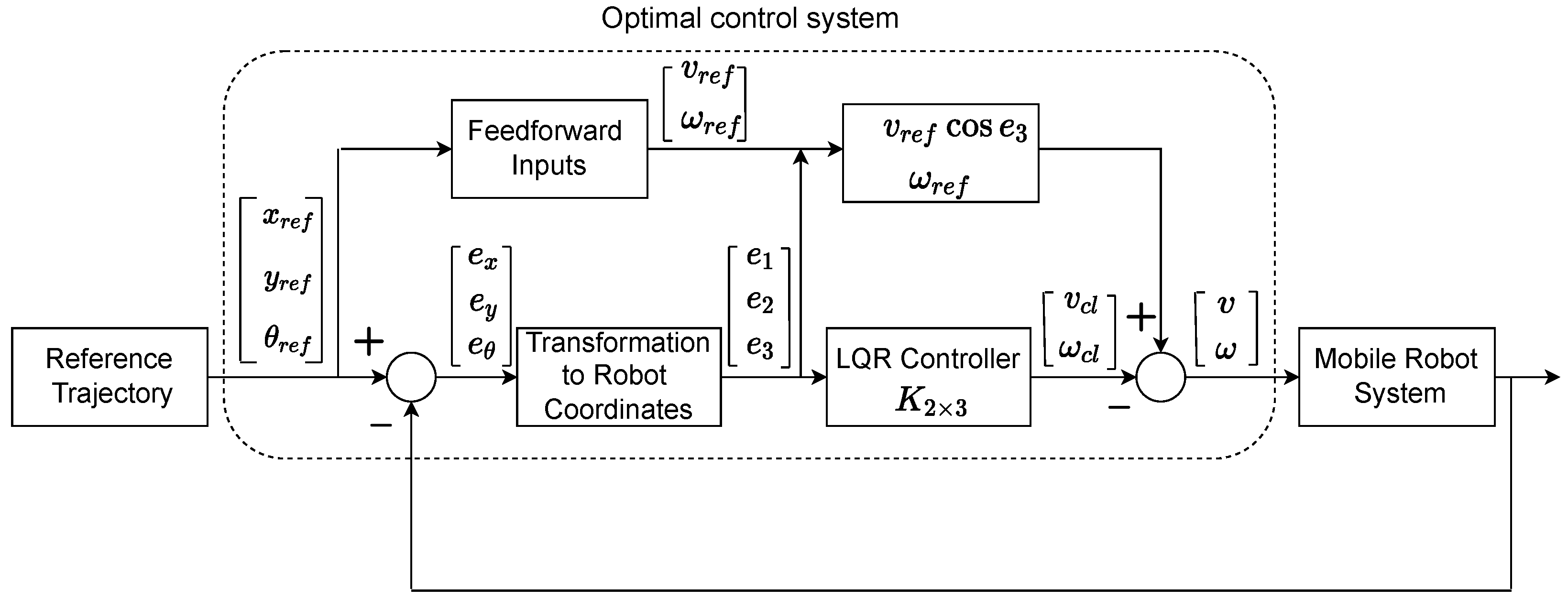
In this section, we detail the design of the linear quadratic regulator (LQR) tracking controller used for controlling the non-holonomic robots, so that they follow a desired trajectory through a leader–follower strategy. A similar design is detailed in [52] for a single robot following a reference trajectory. LQR is an optimal control technique which considers the states of the system and control inputs when making optimal control decisions and computes the state feedback control gain [53]. LQR was chosen because of its simplicity and ease of implementation, while providing good accuracy, as shown in [52] for a single AGV. The designed LQR is a simple controller in comparison with non-linear controllers such as a sliding controller, which has been widely used for AGVs in recent years. As shown in Figure 2, the kinematic controller (LQR controller) generates two control signals, the angular velocity ( ω c l ) and the linear velocity ( v c l ), for each robot’s trajectory tracking. The current position of the robot (x, y, and θ ) is compared with its expected reference trajectory ( x r e f , y r e f and θ r e f ) and the trajectory tracking errors are fed to the LQR controller after the required transformations [52].
To design the LQR controller, let us consider a linear time-invariant (LTI) system:
x ˙ = A x ( t ) + B u ( t ) , t 0 , x ( 0 ) = 0 y ˙ = C x ( t ) + D u ( t ) , t 0
where A R n × n , B R n × m , C R p × n , and D R p × m are the system matrix, control matrix, output matrix, and feed forward matrix, respectively, representing the state space model. The dimensions of these matrices are depicted with n state variables, m inputs, and p outputs. x is the state vector, u is the control vector, and y is the output vector. The LQR controller generates the control input that minimizes the cost function [54] given by Equation (6).
J ( u ) = 0 [ x T ( t ) Q x ( t ) + u T ( t ) R u ( t ) ] d t
where Q = Q T is a positive semi-definite matrix that penalizes the departure of system states from the equilibrium, and R = R T is a positive definite matrix that penalizes the control input [55]. The feedback control law that minimizes the value of the cost function is given by Equation (7):
u = K x
where K, the optimal state feedback control gain matrix, is obtained with Equation (8):
K = R 1 B T P
and P is found by solving the algebraic Riccati Equation (ARE) (9) [56]:
A T P + P A + Q P B R 1 B T P = 0
Thus, to design an LQR controller, the trajectory tracking problem should be written in the form of Equation (5). This gives the trajectory tracking errors in the form of Equation (10).
e x e y e θ = x r e f x y r e f y θ r e f t h e t a
where e x , e y , and e θ are errors in x, y, and heading angle, respectively. To transform these errors into robot coordinates, a rotation matrix was applied to the system as stated in Equation (11).
e 1 e 2 e 3 = cos θ sin θ 0 sin θ cos θ 0 0 0 1 . e x e y e θ
The transformed errors ( e 1 , e 2 , e 3 ) are fed to the LQR controller and it generates the required control signals ω c l and v c l , as shown in Figure 2.
Applying Equation (1) to the time derivative of Equation (11) yields the state space model given by Equation (12).
e 1 ˙ e 2 ˙ e 3 ˙ = cos e 3 0 sin e 3 0 0 1 . v r e f ω r e f + 1 e 2 0 e 1 0 1 . v ω
where
v s . = v r e f cos e 3 v c l ω = ω r e f ω c l
Applying Equation (13) to Equation (12) results in
e 1 ˙ e 2 ˙ e 3 ˙ = 0 ω 0 ω 0 0 0 0 0 . e 1 e 2 e 3 + 0 sin e 3 0 . v r e f + 1 0 0 0 0 1 . v c l ω c l
Linearizing Equation (14) around the operating point ( e 1 = e 2 = e 3 = 0 , v c l = ω c l = 0 ) [51], the state space model of the linear system given by Equation (15) is obtained.
e 1 ˙ e 2 ˙ e 3 ˙ = 0 ω r e f 0 ω r e f 0 v r e f 0 0 0 . e 1 e 2 e 3 + 1 0 0 0 0 1 . v c l ω c l
Comparing Equation (15) with the standard form in Equation (5), the system is controllable if and only if its controllability matrix (R = [ B , A B , A 2 B ]) has a full rank. However, rank (R) = 3 if either v r e f or ω r e f are non-zero, which is a sufficient condition only when the reference inputs v r e f and ω r e f are constant. This happens only when the trajectory is a line or a circular path. The controllability of a driftless system can be derived from Chow’s theorem if the system is completely non-holonomic [51]. The robot model represented by Equation (1) is completely non-holonomic since it has only one non-holonomic constraint, which is represented by Equation (16):
x ˙ sin θ y ˙ cos θ = 0
Therefore, the robot cannot move in a lateral direction due to its wheels and it is controllable [51], as shown in Figure 2, where the LQR controller is given by Equation (17) and K 2 × 3 is the gain matrix with three states and two inputs.
v c l ω c l = k 11 k 12 k 13 k 21 k 22 k 23 . e 1 e 2 e 3
To obtain the LQR controller gain ( K 2 × 3 ), matrices Q and R are tuned, where Q is a positive-definite/semi-definite diagonal matrix related to the state variables, and R is a positive-definite diagonal matrix related to the input variables [57]. The following Q and R were selected according to [52] for the evaluation of our tracking system.
Q = 1 0 0 0 1 0 0 0 10 , R = 0.0001 1 0 0 1

5. Formation Control under Packet Loss

In this section, we first evaluate the controller’s performance under various packet loss conditions. Following that, we discuss the application of an LSTM model to a follower in order to predict the position of the leader when packet loss occurs.

5.1. Impact of Packet Loss on Formation Control

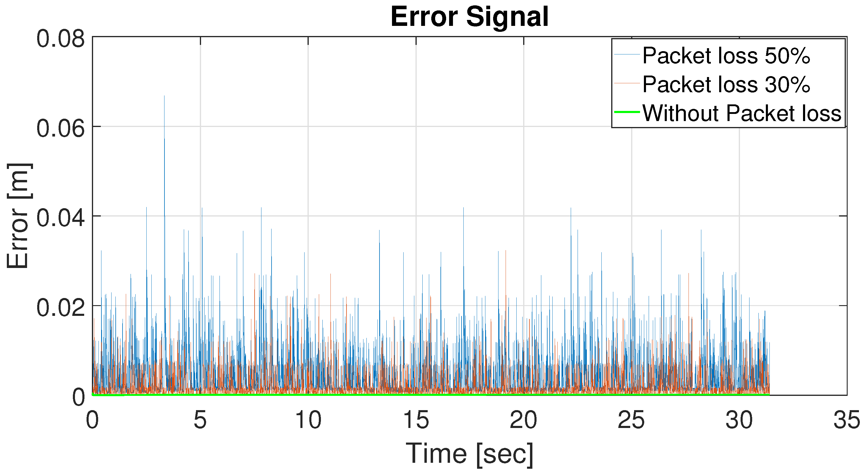
As demonstrated in [52], the LQR controller performs admirably in tracking the trajectory of a single robot along a variety of paths. Here, we extend the LQR tracking control problem [52] to the formation control of multiple robots in various packet loss scenarios. In the leader–follower approach, the leader’s position is communicated to all followers at regular intervals. The communication interval is considered to be 0.05 s and the sampling interval is 0.005 s. The effects of packet loss are depicted in Figure 3, which illustrates how packet loss results in an increased follower position error of around 4 cm. The simulation results in Figure 3 were obtained by considering a memory element in each follower robot that stores the most recent position of the leader. That is, whenever packet loss occurs, a follower makes use of the last received data stored in its memory to track the reference (leader) trajectory. This approach is called MCP, as detailed in Section 2. Here, we apply an LSTM prediction model to alleviate the impact of packet loss and we compare the system’s performance with MCP and GRU.

5.2. Long Short-Term Memory to Cope with Packet Loss

Our objective is to enhance the optimal control system (as shown in Figure 2) using LSTM rather than designing a highly non-linear tracking controller. We believe that, with the recent advancements in machine learning techniques, the existing industrial controller’s performance can be improved in the presence of various network uncertainties such as packet loss, delays, etc. We propose to use LSTM, a type of recurrent network that reuses previously stored data and its dependencies, for predicting the latest position of the reference trajectory (leader). LSTM has been widely used for the prediction of time series data [58,59,60]. As we are attempting to predict the leader’s trajectory, which is a time-based ordered sequence of locations, this problem fits within the LSTM framework. LSTM has been addressed in numerous articles [61,62,63] in order to learn and remember long-term dependency and information. By incorporating various gates, such as an input gate, an output gate, and a forget gate, LSTM is expected to improve traditional recurrent neural networks (RNNs). These various gates enable LSTM to achieve a trade-off between the current and the previous inputs while alleviating an RNN’s vanishing gradient and exploding gradient problems [61]. We detail the LSTM model along with various gates/parameters and evaluate the system’s performance in the following sections.

5.2.1. Architecture of LSTM Prediction and Control

A basic LSTM network for prediction begins with an input layer, followed by an LSTM layer, a fully connected layer, and finally, a regression output layer. The input layer provides the position of the leader to the LSTM layer. The hidden layer is in charge of storing and remembering the position data received from the leader. The output layer provides the leader robot’s predicted position. Since the position of the leader is characterized by its x and y position and heading angle, we use three independent LSTM neural network models for predicting each of these states.
As illustrated in Figure 4, LSTM is equipped with a “gate” structure that enables it to add or remove cell state information and selectively pass the information while passing through different gates as detailed below [61]:
  • Forget gate: The forget gate ( f t ), given by Equation (18), decides whether the information from the previous cell state C t 1 should be discarded or not.
    f t = σ ( W f . [ h t 1 , x t ] + b f )
    where f t is the forget gate, σ is the sigmoid function, W f is the weight matrix, b f is the bias term, h t 1 is the previous hidden layer output, and x t is the new input.
  • Input gate: This gate determines the information that has to be stored in the cell states that includes two parts given by Equation (19). The first part in Equation (19) consisting of σ identifies which value is to be updated, and the second part in Equation (19) including tanh generates the new candidate values.
    i t = σ ( W i . [ h t 1 , x t ] + b i ) C t ˜ = tanh ( W C . [ h t 1 , x t ] + b C )
    where i t is the input gate, C t ˜ is the candidate state of the input, and σ and tanh are the sigmoid and hyperbolic tangent functions, respectively. W i and W C are the weight matrices, b i and b C are the bias terms, h t 1 is the previous hidden layer output, and x t is the new input.
  • Updating cell state: Updating the cell state considers the new candidate memory and the long-term memory given by Equation (20).
    C t = f t × C t 1 + i t × C t ˜
    where C t and C t 1 are the current and previous memory states, f t is the forget gate, i t is the input gate, and C t ˜ is the input candidate state.
  • Output gate: This gate determines the output of the LSTM given by Equation (21).
    o t = σ ( W o . [ h t 1 , x t ] + b o ) h t = o t × tanh C t
    where o t is the output gate. W o and b o are the weight matrix and bias terms, respectively. h t 1 and h t are the previous and current hidden layer outputs, x t is the new input, and C t is the current state of the memory block. The first part in Equation (21), which includes σ , determines which part of the cell state will be output ( o t ), and the second part in Equation (21) processes the cell state by tanh multiplied by the output of the sigmoid layer.

5.2.2. Application of LSTM for Leader Position Prediction

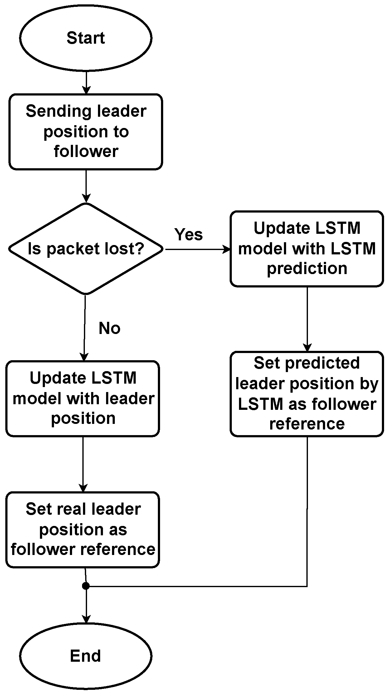
As previously stated, follower robots should have access to the latest position of the leader in order to maintain accurate formation control. When packet loss occurs, followers are unaware of the leader’s true position. To cope with this, we use an LSTM for predicting the leader’s trajectory. The LSTM network is trained using the leader trajectory and then its states are updated.
As shown in Figure 5, when no packets are lost, network states are updated with the actual observed leader position. In the event of packet loss, network states are updated using previous LSTM predictions, as observed leader position values are unavailable.

6. Performance Evaluation

In this section, we evaluate the performance of the different prediction schemes LSTM, GRU, and MCP. We also evaluate the performance of the leader–follower formation control system with these prediction methods in different packet loss scenarios. All the performance evaluations are carried out through MATLAB/SIMULINK simulations.

6.1. Prediction Accuracy of LSTM, GRU, and MCP

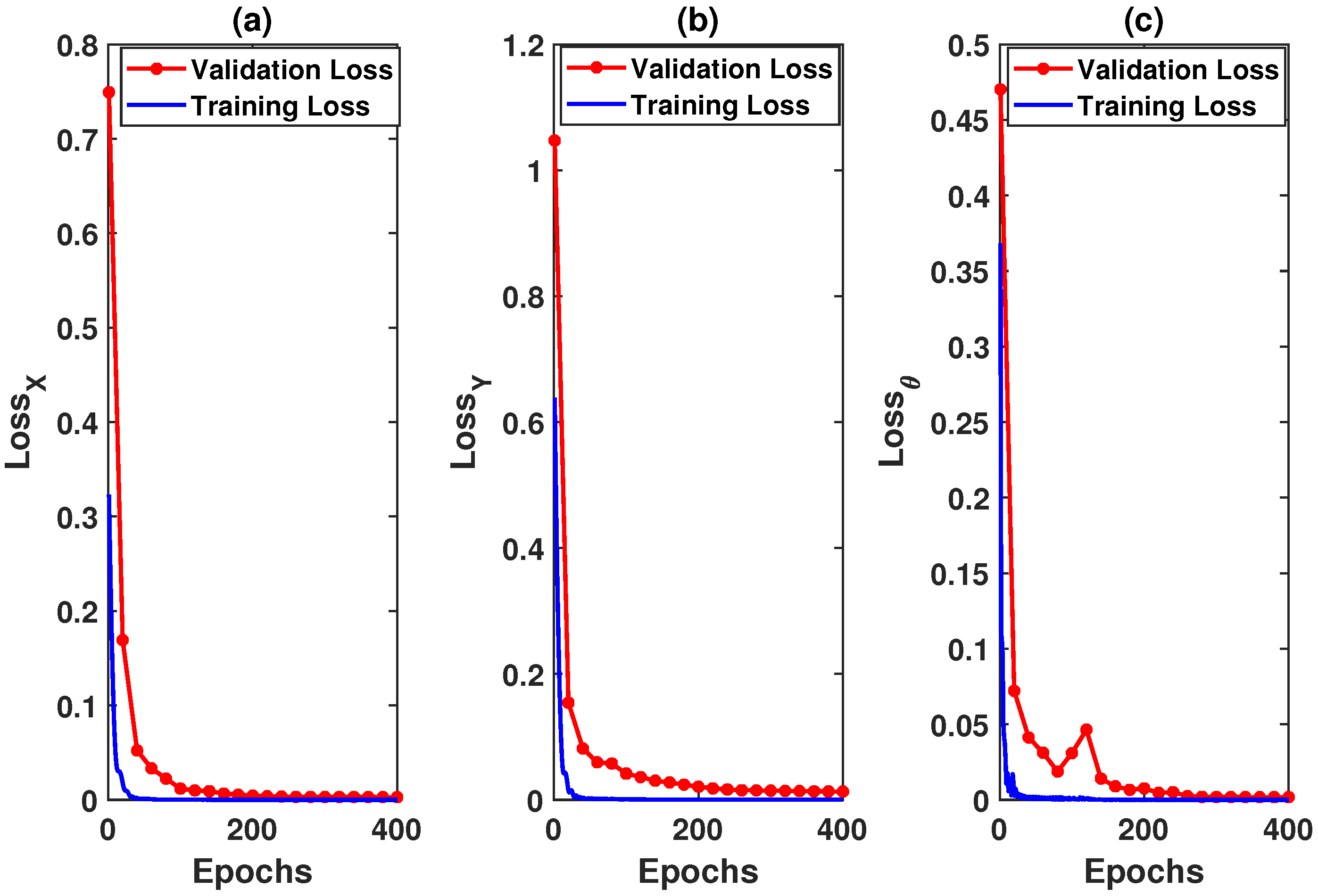
Here, we discuss the prediction performance of LSTM, GRU, and MCP for a circular trajectory for 30 % and 50 % packet loss. LSTM was trained with the leader’s trajectory positions; 80% of these data were used for training the LSTM and 20% was used for validation. Figure 6 shows the validation and training loss for LSTM. Over the 400 time periods, the proposed LSTM model was able to learn to predict with the desired accuracy.
The errors between the actual and the predicted positions of the leader trajectory (X, Y, and heading angle) are shown in Figure 7. As shown in the figure, LSTM provided more accurate predictions than GRU and MCP. The root mean square error (RMSE) between the actual and predicted positions is shown in Table 1. From Table 1, it is clear that LSTM provided the most accurate prediction in comparison with GRU and MCP for both 30% and 50% packet loss scenarios. MCP had the worst prediction performance.

6.2. Simulation Results

Here, we discuss the formation control performance of four robots with one of them acting as leader. For each robot, the controller diagram depicted in Figure 2 was simulated using MATLAB/SIMULINK. The followers and the leader attempted to maintain their formation as they travelled along a pre-defined path. At regular communication intervals, the leader’s position was communicated to all the followers via wireless broadcast communication. In the event of packet loss, LSTM predicted the leader’s position for the followers. The LSTM and GRU model settings were identical and they are listed in Table 2. The LSTM and GRU model parameters were carefully chosen to maintain a balance among prediction accuracy, computing resources, and calculation time.
In our use case, the follower robot was expected to maintain a predefined distance from the leader. The accuracy of the LSTM location prediction was measured using the RMSE given by Equation (22). RMSE is a frequently used measure of the difference between the predicted and the actually observed values.
R M S E = 1 N i = 1 N ( x i x ^ i ) 2
where x i is the observed value, x ^ i is the predicted value, and N is the number of data points.
The simulations were carried out with a sampling time of 5 ms and a communication interval of 50 ms. The leader positions communicated to the followers were vulnerable to packet loss, which was modelled using a Bernoulli distribution with a probability of ρ equal to 0.3 and 0.5. Packet loss had a more significant impact on the formation control when the trajectory followed was not simple in nature (e.g., straight line or its variants). We chose circular and eight-shaped paths for our evaluations.

6.2.1. Circular Path

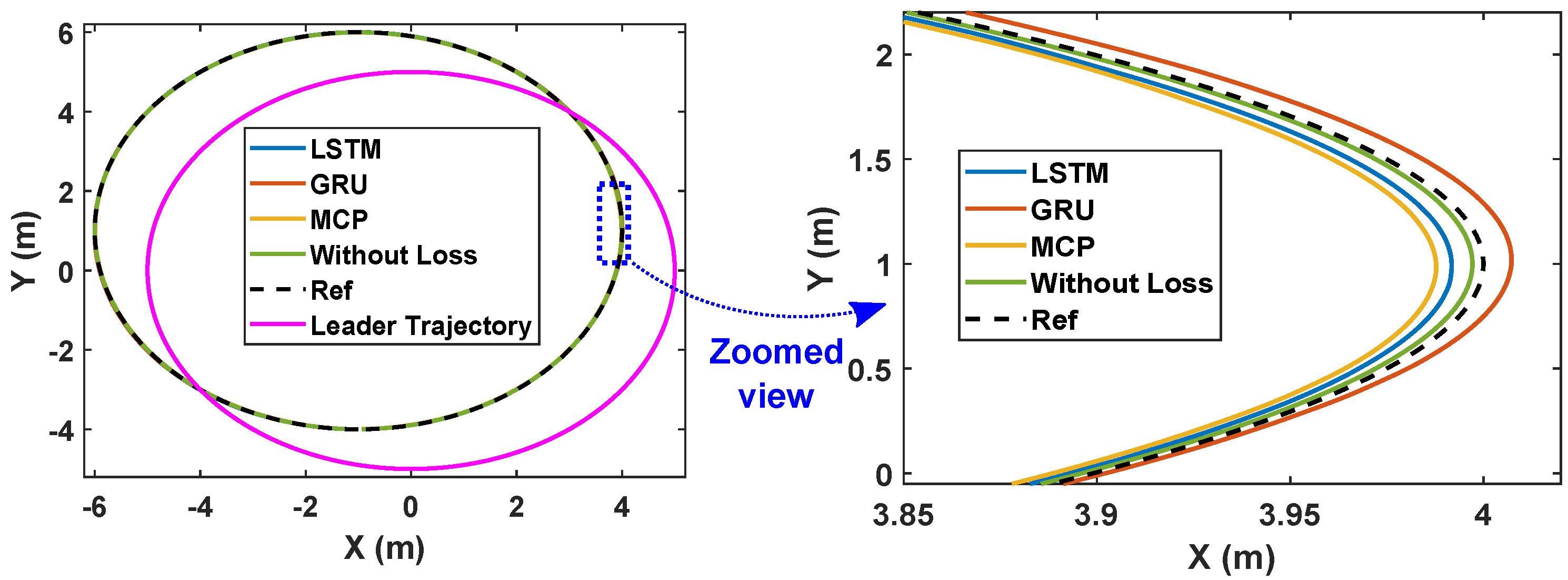
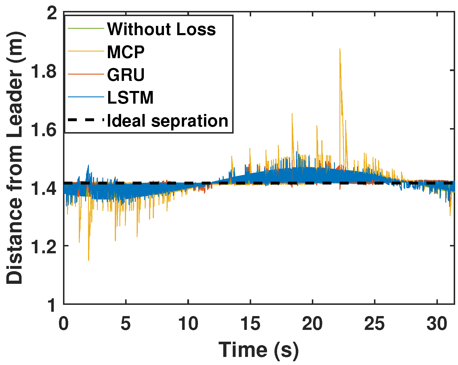
Here, we consider the leader and the followers as moving through a circle while packet loss is considered to be 30%. As illustrated in Figure 8, LSTM prediction compensated for packet loss better than GRU and MCP. The distance from the leader is also depicted in Figure 9, which compares the prediction performance of MCP to those of LSTM and GRU. The RMSE values of X, Y, and the heading angle of the follower are shown in Table 3. From Figure 8, it is clear that LSTM-based prediction can provide formation control performance that is comparable to that in perfect communication scenarios (0% packet loss), even with 30% packet loss. This is clearly observed in the RMSE as well. A lower RMSE for X and a close enough RMSE for Y and heading angle can be observed in Table 3 when comparing 0% and 30% packet loss scenarios. This demonstrates how well LSTM prediction can compensate for packet loss. Overall, LSTM performed 10% better than GRU and 148.07% better than MCP.
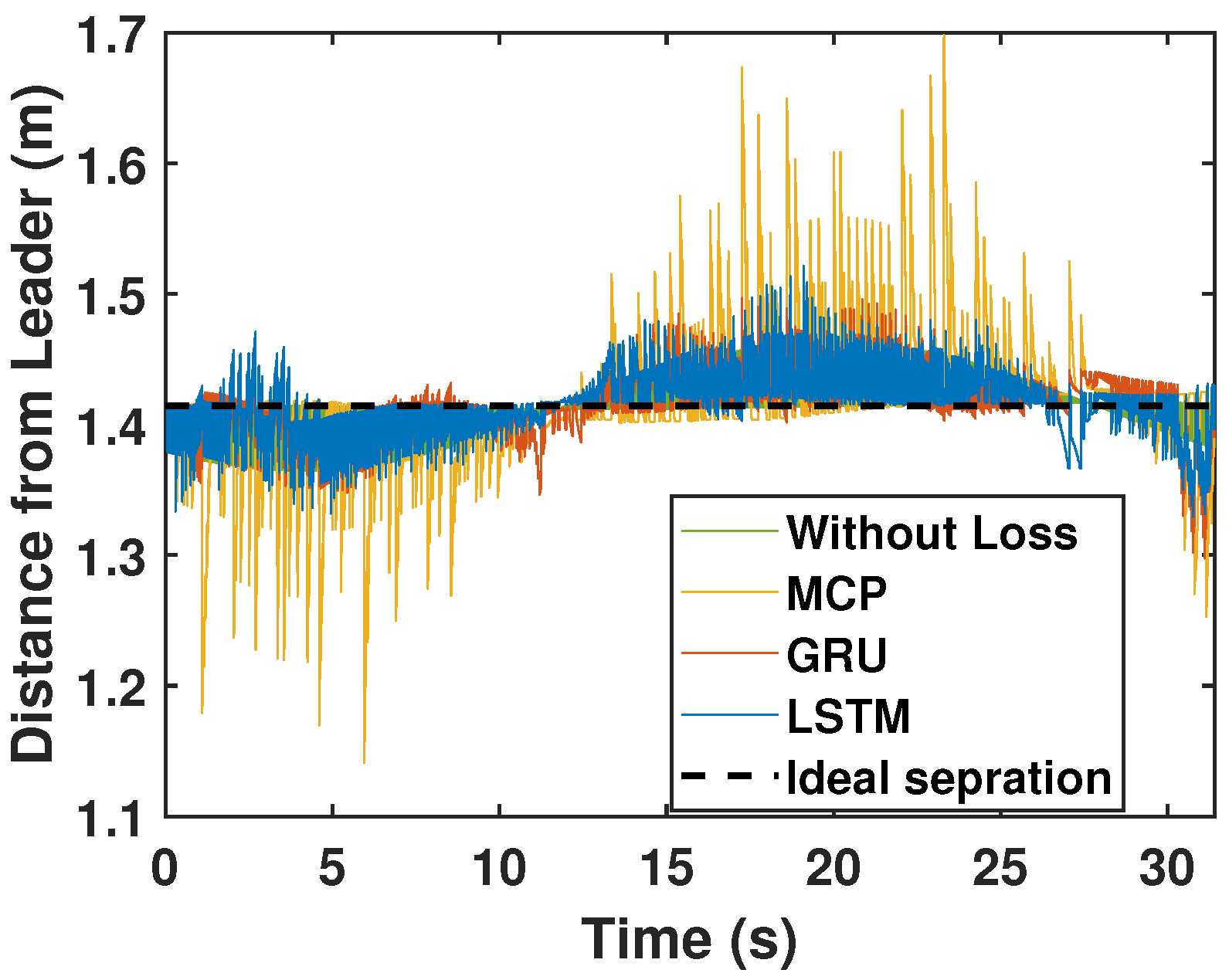
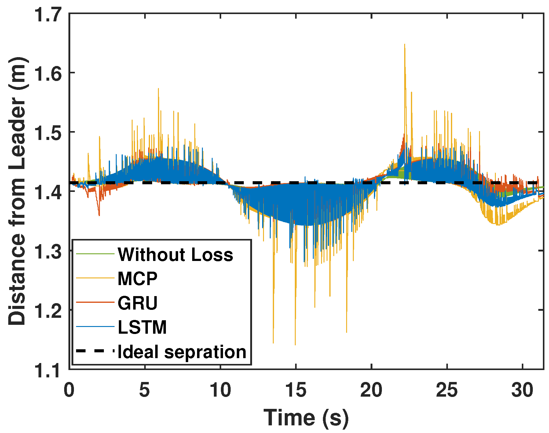
We repeated the circular trajectory scenario with a 50% packet loss. The follower performance is illustrated in Figure 10. LSTM again outperformed GRU and MCP in terms of prediction. The distance from the leader is depicted in Figure 11 and the MCP’s performance is compared to those of LSTM and GRU. RMSE was calculated for the X and Y positions and the heading angle of the follower in Table 3 for a 50% packet loss. Here, LSTM outperformed GRU and MCP; while packet loss was 50%, LSTM performance was only slightly worse than it was with 0% loss. Overall, LSTM performed 21.41% better than GRU and 223.17% better than MCP.

6.2.2. Eight-Shaped Trajectory

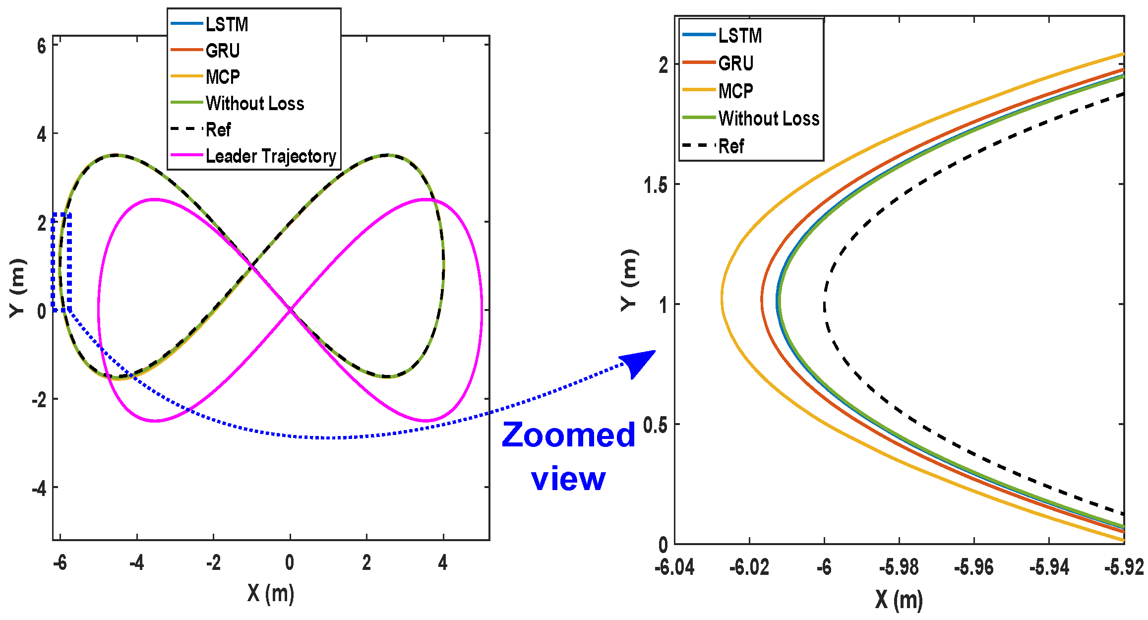
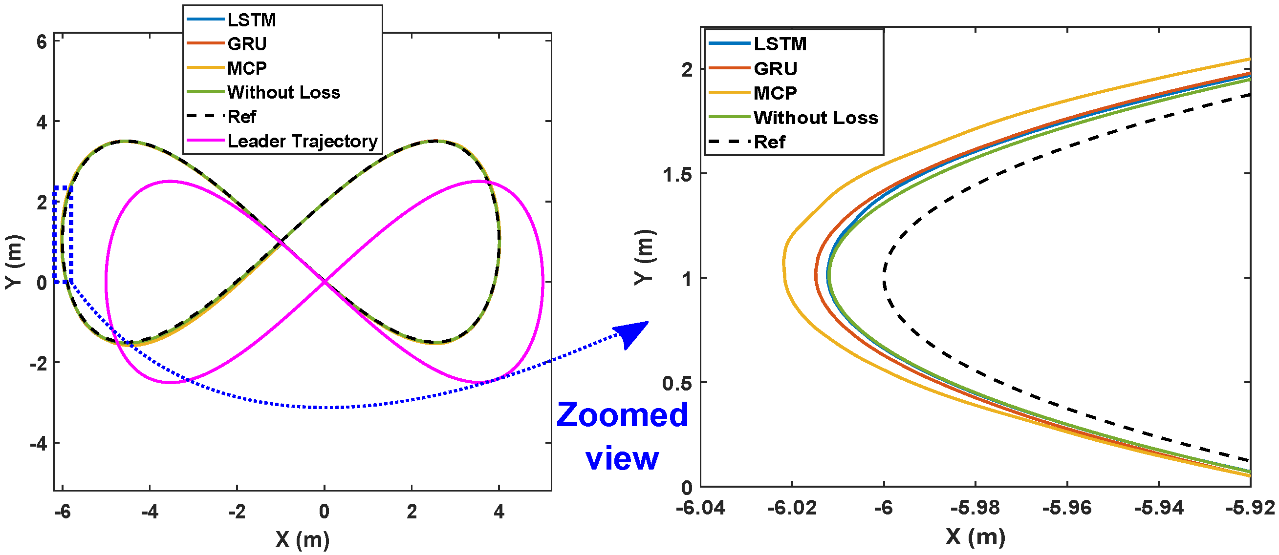
Here, we detail the formation control performance of the leader and the followers while following an eight-shaped trajectory in different packet loss scenarios. Figure 12 shows the system’s performance while the packet loss was 30%. It is clearly visible that the LSTM prediction was very close to the perfect communication scenarios when compared with GRU and MCP. The distance from the leader is depicted in Figure 13. Table 4 gives the RMSE for the X, Y, and heading angle of the followers. LSTM performance (RMSE of X, Y, and heading angle) while having 30% packet loss was even better than it was in the perfect communication scenarios (0% packet loss). This demonstrates that LSTM prediction can completely compensate for packet loss and even compensate for the quantization error in the leader positions due to discrete communication intervals. Overall, LSTM performed 5.20% better than GRU and 156.14% better than MCP.
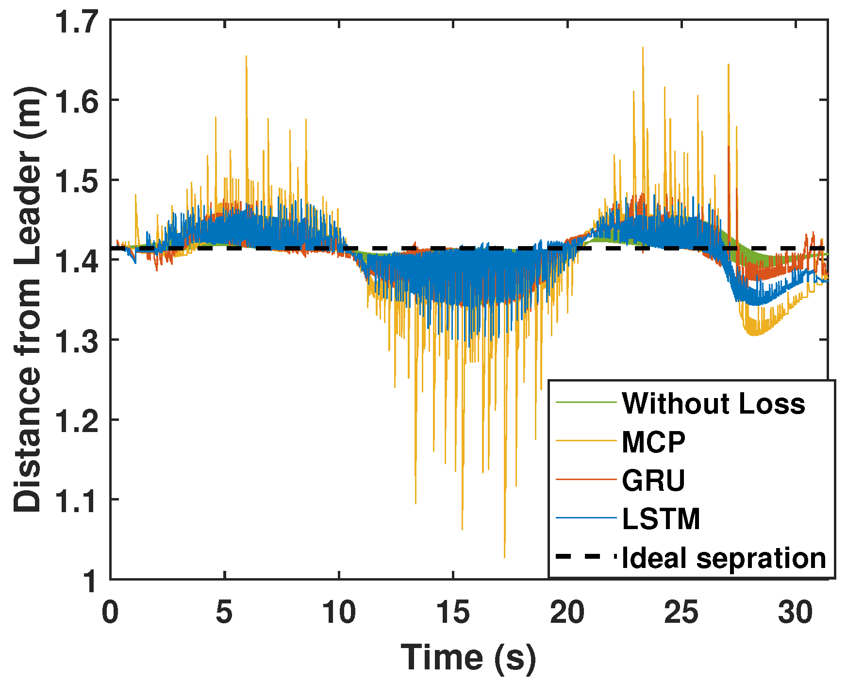
The formation control experiment along the eight-shaped trajectory was repeated with 50% packet loss. As illustrated in Figure 14, LSTM again outperformed GRU and MCP in terms of prediction. The distance from the leader is depicted in Figure 15. MCP had a weaker performance compared to LSTM and GRU. The RMSE for the X, Y, and heading angle of the follower is presented in Table 4 for the 50% packet loss scenario. As observed earlier, LSTM outperformed GRU and MCP. LSTM’s prediction performance is comparable with that in a perfect communication scenario (0% packet loss) even when sustaining 50% packet loss. Overall, LSTM performed 14.49% better than GRU and 250.53% better than MCP.

7. Conclusions

The formation control problem of non-holonomic AGVs is presented in this study. Decentralized formation control of multiple AGVs is presented based on leader-follower formation control by an LQR controller. The performance of the LQR controller is analyzed when sustaining packet loss and with packet loss compensation using an LSTM neural network model. The LSTM algorithm is in charge of forecasting the leader’s position based on the previous leader’s position. When packet loss occurs, followers rely on LSTM-generated predicted position values to maintain their formation accurately. Numerous simulations were run to compare the performance of the LSTM to that of MCP and GRU. LSTM prediction significantly aids in compensating for packet loss along a variety of trajectories. Overall, LSTM performs 12% better than GRU and 194% better than MCP. In future research, we will consider communication delay and other details of connectivity aspects and plan to also implement our proposed approach in a physical robot test environment.

Author Contributions

L.S. performed theoretical investigation and simulations and contributed to the paper. J.J. and M.N.-A.-R. contributed to the theoretical investigation and the manuscript. D.P. contributed to the theoretical investigation and the manuscript and supervised the work overall. All authors have read and agreed to the published version of the manuscript.

Funding

This publication has emanated from research conducted in part with the financial support of Science Foundation Ireland under Grant number 16/RC/3918 (CONFIRM Centre for Smart Manufacturing).

Conflicts of Interest

The authors declare no conflict of interest.

References

  1. Javed, M.A.; Muram, F.U.; Punnekkat, S.; Hansson, H. Safe and secure platooning of Automated Guided Vehicles in Industry 4.0. J. Syst. Archit. 2021, 121, 102309. [Google Scholar] [CrossRef]
  2. Soni, A.; Hu, H. A multi-robot simulator for the evaluation of formation control algorithms. In Proceedings of the 11th Computer Science and Electronic Engineering (CEEC), Essex, UK, 18–20 September 2019; pp. 79–84. [Google Scholar]
  3. Chen, Y.Q.; Wang, Z. Formation control: a review and a new consideration. In Proceedings of the 2005 IEEE/RSJ International Conference on Intelligent Robots and Systems, Edmonton, AB, Canada, 2–6 August 2005; pp. 3181–3186. [Google Scholar]
  4. Wang, S.; Jiang, L.; Meng, J.; Xie, Y.; Ding, H. Training for smart manufacturing using a mobile robot-based production line. Front. Mech. Eng. 2021, 16, 249–270. [Google Scholar] [CrossRef]
  5. Feng, S.; Zhang, Y.; Li, S.E.; Cao, Z.; Liu, H.X.; Li, L. String stability for vehicular platoon control: Definitions and analysis methods. Annu. Rev. Control 2019, 47, 81–97. [Google Scholar] [CrossRef]
  6. Rizzo, C.; Lagraña, A.; Serrano, D. Geomove: Detached agvs for cooperative transportation of large and heavy loads in the aeronautic industry. In Proceedings of the 2020 IEEE International Conference on Autonomous Robot Systems and Competitions (ICARSC), Ponta Delgada, Portugal, 15–16 April 2020; pp. 126–133. [Google Scholar]
  7. Liu, A.; Zhang, W.A.; Yu, L.; Yan, H.; Zhang, R. Formation control of multiple mobile robots incorporating an extended state observer and distributed model predictive approach. IEEE Trans. Syst. Man Cybern. Syst. 2018, 50, 4587–4597. [Google Scholar] [CrossRef]
  8. Madhevan, B.; Sreekumar, M. Analysis of Communication Delay and Packet Loss During Localization Among Mobile Robots. In Intelligent Systems Technologies and Applications; Springer: Berlin, Germany, 2016; pp. 3–12. [Google Scholar]
  9. Pratama, P.S.; Nguyen, T.H.; Kim, H.K.; Kim, D.H.; Kim, S.B. Positioning and obstacle avoidance of automatic guided vehicle in partially known environment. Int. J. Control Autom. Syst. 2016, 14, 1572–1581. [Google Scholar] [CrossRef]
  10. Hu, J.; Zhang, H.; Liu, L.; Zhu, X.; Zhao, C.; Pan, Q. Convergent multiagent formation control with collision avoidance. IEEE Trans. Robot. 2020, 36, 1805–1818. [Google Scholar] [CrossRef]
  11. Consolini, L.; Morbidi, F.; Prattichizzo, D.; Tosques, M. Leader–follower formation control of nonholonomic mobile robots with input constraints. Automatica 2008, 44, 1343–1349. [Google Scholar] [CrossRef]
  12. Wang, C.; Tnunay, H.; Zuo, Z.; Lennox, B.; Ding, Z. Fixed-time formation control of multirobot systems: Design and experiments. IEEE Trans. Ind. Electron. 2018, 66, 6292–6301. [Google Scholar] [CrossRef] [Green Version]
  13. Nandanwar, A.; Dhar, N.K.; Malyshev, D.; Rybak, L.; Behera, L. Stochastic Event-Based Super-Twisting Formation Control for Multi-Agent System under Network Uncertainties. IEEE Trans. Control Netw. Syst. 2021. [Google Scholar] [CrossRef]
  14. Bai, C.; Yan, P.; Pan, W.; Guo, J. Learning-based multi-robot formation control with obstacle avoidance. IEEE Trans. Intell. Transp. Syst. 2021. [Google Scholar] [CrossRef]
  15. Lin, S.; Jia, R.; Yue, M.; Xu, Y. On composite leader–follower formation control for wheeled mobile robots with adaptive disturbance rejection. Appl. Artif. Intell. 2019, 33, 1306–1326. [Google Scholar] [CrossRef]
  16. Peng, Z.; Yang, S.; Wen, G.; Rahmani, A.; Yu, Y. Adaptive distributed formation control for multiple nonholonomic wheeled mobile robots. Neurocomputing 2016, 173, 1485–1494. [Google Scholar] [CrossRef]
  17. Cepeda-Gomez, R.; Perico, L.F. Formation control of nonholonomic vehicles under time delayed communications. IEEE Trans. Autom. Sci. Eng. 2015, 12, 819–826. [Google Scholar] [CrossRef] [Green Version]
  18. Wang, L.; Liu, Q.; Zang, C.; Zhu, S.; Gan, C.; Liu, Y. Formation Control of Dual Auto Guided Vehicles Based on Compensation Method in 5G Networks. Machines 2021, 9, 318. [Google Scholar] [CrossRef]
  19. Santos, C.; Espinosa, F.; Martinez-Rey, M.; Gualda, D.; Losada, C. Self-triggered formation control of nonholonomic robots. Sensors 2019, 19, 2689. [Google Scholar] [CrossRef] [Green Version]
  20. Wei, H.; Lv, Q.; Duo, N.; Wang, G.; Liang, B. Consensus algorithms based multi-robot formation control under noise and time delay conditions. Appl. Sci. 2019, 9, 1004. [Google Scholar] [CrossRef] [Green Version]
  21. Peng, L.; Guan, F.; Perneel, L.; Fayyad-Kazan, H.; Timmerman, M. Decentralized multi-robot formation control with communication delay and asynchronous clock. J. Intell. Robot. Syst. 2018, 89, 465–484. [Google Scholar] [CrossRef]
  22. Liu, Y.; Candell, R.; Moayeri, N. Effects of wireless packet loss in industrial process control systems. ISA Trans. 2017, 68, 412–424. [Google Scholar] [CrossRef] [Green Version]
  23. Teh, X.X.; Aijaz, A.; Portelli, A.; Jones, S. Communications-based Formation Control of Mobile Robots: Modeling, Analysis and Performance Evaluation. In Proceedings of the 23rd International ACM Conference on Modeling, Analysis and Simulation of Wireless and Mobile Systems, Alicante, Spain, 16–20 November 2020; pp. 149–153. [Google Scholar]
  24. Elahi, A.; Alfi, A.; Modares, H. H consensus control of discrete-time multi-agent systems under network imperfections and external disturbance. IEEE/CAA J. Autom. Sin. 2019, 6, 667–675. [Google Scholar] [CrossRef]
  25. Wu, J.; Chen, X.; Liu, A.; Yu, L. Predictive control for visual servoing control of cyber physical systems with packet loss. Peer-to-Peer Netw. Appl. 2019, 12, 1774–1784. [Google Scholar] [CrossRef]
  26. Phung, M.D.; Tran, T.H.; Tran, Q.V. Stable control of networked robot subject to communication delay, packet loss, and out-of-order delivery. Vietnam. J. Mech. 2014, 36, 215–233. [Google Scholar] [CrossRef] [Green Version]
  27. Wang, B.F.; Guo, G. Kalman filtering with partial Markovian packet losses. Int. J. Autom. Comput. 2009, 6, 395–400. [Google Scholar] [CrossRef]
  28. Abdellah, A.R.; Mahmood, O.A.; Koucheryavy, A. Delay prediction in IoT using machine learning approach. In Proceedings of the 12th International Congress on Ultra Modern Telecommunications and Control Systems and Workshops (ICUMT), Online, 5–7 October 2020; pp. 275–279. [Google Scholar]
  29. Abdellah, A.R.; Koucheryavy, A. Deep learning with long short-term memory for iot traffic prediction. In Internet of Things, Smart Spaces, and Next Generation Networks and Systems; Springer: Berlin, Germany, 2020; pp. 267–280. [Google Scholar]
  30. Graves, A. Long short-term memory. In Supervised Sequence Labelling with Recurrent Neural Networks; Springer: Berlin, Germany, 2012; pp. 37–45. [Google Scholar]
  31. Manaswi, N.K. Rnn and lstm. In Deep Learning with Applications Using Python; Springer: Berlin, Germany, 2018; pp. 115–126. [Google Scholar]
  32. Mirali, F.; Werner, H. A Dynamic Quasi-Taylor Approach for Distributed Consensus Problems with Packet Loss. In Proceedings of the 2020 American Control Conference (ACC), Denver, CO, USA, 1–3 July 2020; pp. 701–706. [Google Scholar]
  33. Zhang, T.Y.; Liu, G.P. Tracking control of wheeled mobile robots with communication delay and data loss. J. Syst. Sci. Complex. 2018, 31, 927–945. [Google Scholar] [CrossRef]
  34. Fu, R.; Zhang, Z.; Li, L. Using LSTM and GRU neural network methods for traffic flow prediction. In Proceedings of the 2016 31st Youth Academic Annual Conference of Chinese Association of Automation (YAC), Wuhan, China, 11–13 November 2016; pp. 324–328. [Google Scholar]
  35. Tian, B.; Wang, G.; Xu, Z.; Zhang, Y.; Zhao, X. Communication delay compensation for string stability of CACC system using LSTM prediction. Veh. Commun. 2021, 29, 100333. [Google Scholar] [CrossRef]
  36. Al Issa, S.; Kar, I. Design and implementation of event-triggered adaptive controller for commercial mobile robots subject to input delays and limited communications. Control Eng. Pract. 2021, 114, 104865. [Google Scholar] [CrossRef]
  37. Gong, X.; Pan, Y.J.; Pawar, A. A novel leader following consensus approach for multi-agent systems with data loss. Int. J. Control Autom. Syst. 2017, 15, 763. [Google Scholar] [CrossRef]
  38. Zhang, T.; Li, J. Iterative Learning Control for Multi-Agent Systems with Finite-Leveled Sigma-Delta Quantizer and Input Saturation. In Proceedings of the 2021 40th Chinese Control Conference (CCC), Shanghai, China, 26–28 July 2021; pp. 5637–5644. [Google Scholar]
  39. Wu, Y.; Zhang, J.; Ge, Y.; Sheng, Z.; Fang, Y. A Dropout Compensation ILC Method for Formation Tracking of Heterogeneous Multi-Agent Systems with Loss of Multiple Communication Packets. Appl. Sci. 2020, 10, 4752. [Google Scholar] [CrossRef]
  40. Bristow, D.A.; Tharayil, M.; Alleyne, A.G. A survey of iterative learning control. IEEE Control Syst. Mag. 2006, 26, 96–114. [Google Scholar]
  41. Xuhui, B.; Zhongsheng, H.; Shangtai, J.; Ronghu, C. An iterative learning control design approach for networked control systems with data dropouts. Int. J. Robust Nonlinear Control 2016, 26, 91–109. [Google Scholar] [CrossRef]
  42. Deng, X.; Sun, X.; Liu, S. Iterative learning control for leader-following consensus of nonlinear multi-agent systems with packet dropout. Int. J. Control Autom. Syst. 2019, 17, 2135–2144. [Google Scholar] [CrossRef]
  43. Dutton, B.; Maloney, E.S. Dutton’s Navigation & Piloting; Prentice Hall: Upper Saddle River, NJ, USA, 1985. [Google Scholar]
  44. Topini, E.; Topini, A.; Franchi, M.; Bucci, A.; Secciani, N.; Ridolfi, A.; Allotta, B. LSTM-based Dead Reckoning Navigation for Autonomous Underwater Vehicles. In Proceedings of the Global Oceans 2020: Singapore–US Gulf Coast, Biloxi, MS, USA, 5–30 October 2020. [Google Scholar]
  45. Berkeveld, R.A. Design and Implementation of Unicycle AGVs for Cooperative Control. Master’s Thesis, Eindhoven University of Technology, Eindhoven, The Netherlands, 26 September 2016. [Google Scholar]
  46. Yan, T. Positioning of logistics and warehousing automated guided vehicle based on improved LSTM network. Int. J. Syst. Assur. Eng. Manag. 2021, 1–10. [Google Scholar] [CrossRef]
  47. Van Nam, D.; Gon-Woo, K. Deep Learning based-State Estimation for Holonomic Mobile Robots Using Intrinsic Sensors. In Proceedings of the 2021 21st International Conference on Control, Automation and Systems (ICCAS), Jeju, Korea, 12–15 October 2021. [Google Scholar]
  48. Quan, Y.; Huang, L.; Ma, L.; He, Y.; Wang, R. Neural Network-Based Indoor Autonomously-Navigated AGV Motion Trajectory Data Fusion. Autom. Control Comput. Sci. 2021, 55, 334–345. [Google Scholar] [CrossRef]
  49. Çatal, O.; Leroux, S.; De Boom, C.; Verbelen, T.; Dhoedt, B. Anomaly detection for autonomous guided vehicles using bayesian surprise. In Proceedings of the 2020 IEEE/RSJ International Conference on Intelligent Robots and Systems (IROS), Las Vegas, NV, USA, 24 October–24 January 2021. [Google Scholar]
  50. Ding, X.; Zhang, D.; Zhang, L.; Zhang, L.; Zhang, C.; Xu, B. Fault Detection for Automatic Guided Vehicles Based on Decision Tree and LSTM. In Proceedings of the 2021 5th International Conference on System Reliability and Safety (ICSRS), Palermo, Italy, 24–26 November 2021. [Google Scholar]
  51. Klancar, G.; Matko, D.; Blazic, S. Mobile robot control on a reference path. In Proceedings of the 2005 IEEE International Symposium on, Mediterrean Conference on Control and Automation Intelligent Control, Limassol, Cyprus, 27–29 June 2005; pp. 1343–1348. [Google Scholar]
  52. Abbasi, A.; Moshayedi, A.J. Trajectory tracking of two-wheeled mobile robots, using LQR optimal control method, based on computational model of KHEPERA IV. J. Simul. Anal. Nov. Technol. Mech. Eng. 2018, 10, 41–50. [Google Scholar]
  53. Prasad, L.B.; Tyagi, B.; Gupta, H.O. Optimal control of nonlinear inverted pendulum system using PID controller and LQR: Performance analysis without and with disturbance input. Int. J. Autom. Comput. 2014, 11, 661–670. [Google Scholar] [CrossRef] [Green Version]
  54. Kumar, E.V.; Jerome, J. Algebraic Riccati equation based Q and R matrices selection algorithm for optimal LQR applied to tracking control of 3rd order magnetic levitation system. Arch. Electr. Eng. 2016, 65, 151–168. [Google Scholar] [CrossRef] [Green Version]
  55. Desineni, S.N. Optimal control systems. In Electrical Engineering Textbook Series; CRC Press: Boca Raton, FL, USA, 2003. [Google Scholar]
  56. Willems, J. Least squares stationary optimal control and the algebraic Riccati equation. IEEE Trans. Autom. Control 1971, 16, 621–634. [Google Scholar] [CrossRef] [Green Version]
  57. Katsuhiko, O. Modern Control Engineering; Prentice Hall: Upper Saddle River, NJ, USA, 2010. [Google Scholar]
  58. Song, X.; Liu, Y.; Xue, L.; Wang, J.; Zhang, J.; Wang, J.; Jiang, L.; Cheng, Z. Time-series well performance prediction based on Long Short-Term Memory (LSTM) neural network model. J. Pet. Sci. Eng. 2020, 186, 106682. [Google Scholar] [CrossRef]
  59. Du, Y.; Wang, W.; Wang, L. Hierarchical recurrent neural network for skeleton based action recognition. In Proceedings of the IEEE Conference on Computer Vision and Pattern Recognition, Boston, MA, USA, 7–12 June 2015; pp. 1110–1118. [Google Scholar]
  60. Kawakami, K. Supervised Sequence Labelling with Recurrent Neural Networks. Ph.D. Thesis, Technical University of Munich, München, Germany, 2008. [Google Scholar]
  61. Zhang, X.; Zhao, M.; Dong, R. Time-series prediction of environmental noise for urban iot based on long short-term memory recurrent neural network. Appl. Sci. 2020, 10, 1144. [Google Scholar] [CrossRef] [Green Version]
  62. Gers, F.A.; Schmidhuber, J.; Cummins, F. Learning to forget: Continual prediction with LSTM. Neural Comput. 2000, 12, 2451–2471. [Google Scholar] [CrossRef]
  63. Zhang, Q.; Wang, H.; Dong, J.; Zhong, G.; Sun, X. Prediction of sea surface temperature using long short-term memory. IEEE Geosci. Remote Sens. Lett. 2017, 14, 1745–1749. [Google Scholar] [CrossRef] [Green Version]
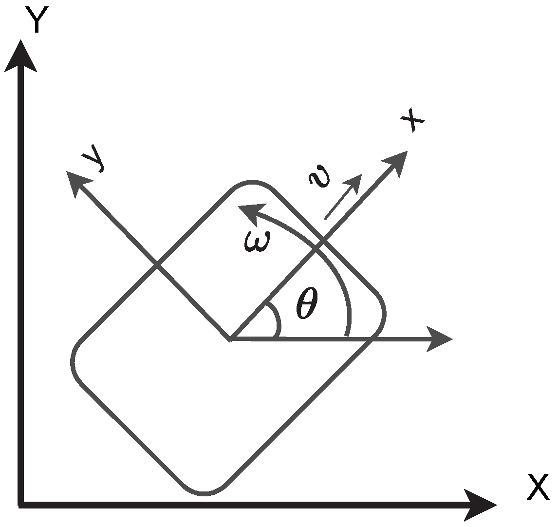
Figure 1. Kinematic model of non-holonomic robot.
Sensors 22 03552 g001
Figure 2. Mobile robot controller.
Sensors 22 03552 g002
Figure 3. Effect of packet loss.
Sensors 22 03552 g003
Figure 4. LSTM architecture.
Sensors 22 03552 g004
Figure 5. The flowchart of the proposed approach of sending the leader position to the follower.
Sensors 22 03552 g005
Figure 6. Training and validation loss for LSTM: (a) loss for X; (b) loss for Y; (c) loss for heading angle.
Sensors 22 03552 g006
Figure 7. Prediction errors: (a) error for X; (b) error for Y; (c) error for heading angle.
Sensors 22 03552 g007
Figure 8. Trajectory of the robots during formation control (packet loss—30%).
Sensors 22 03552 g008
Figure 9. Distance of the follower from the leader for the circular trajectory (packet loss—30%).
Sensors 22 03552 g009
Figure 10. Trajectory of the robots during formation control (packet loss—50%).
Sensors 22 03552 g010
Figure 11. Distance of the follower from the leader for the circular trajectory (packet loss—50%).
Sensors 22 03552 g011
Figure 12. Trajectory of the robots during formation control (packet loss—30%).
Sensors 22 03552 g012
Figure 13. Distance of the follower from the leader for the circular trajectory (packet loss—30%).
Sensors 22 03552 g013
Figure 14. Trajectory of the robots during formation control (packet loss—50%).
Sensors 22 03552 g014
Figure 15. Distance of the follower from the leader for the circular trajectory (packet loss—50%).
Sensors 22 03552 g015
Table 1. RMSE of prediction error.
Packet Loss 30% 50%
RMSEXYHeading AngleXYHeading Angle
LSTM3.19 × 10 2 3.46 × 10 2 9.8 × 10 3 3 × 10 2 3.71 × 10 2 1.01 × 10 2
GRU3.35 × 10 2 3.52 × 10 2 1.17 × 10 2 3.41 × 10 2 3.72 × 10 2 1.43 × 10 2
MCP3.47 × 10 2 4.28 × 10 2 1.10 × 10 2 5.53 × 10 2 5.70 × 10 2 1.59 × 10 2
Table 2. LSTM and GRU model setting.
LSTMXYHeading Angle
Epox400400400
Hidden nodes10107
Batch size128128128
Learning rate0.0050.010.1
Learning rate drop factor0.20.20.2
Table 3. RMSE of follower error for the circle path.
Packet LossPrediction MethodRMSE-XRMSE-YRMSE-Heading Angle
0%-2.76 × 10 2 2.77 × 10 2 7.8 × 10 3
LSTM2.45 × 10 2 2.81 × 10 2 8.3 × 10 2
30%GRU2.55 × 10 2 3.07 × 10 2 9.7 × 10 3
MCP6.23 × 10 2 7.20 × 10 2 1.94 × 10 2
LSTM2.39 × 10 2 3.04 × 10 2 9.1 × 10 3
50%GRU2.60 × 10 2 3.49 × 10 2 1.28 × 10 2
MCP8.94 × 10 2 9.15 × 10 2 2.68 × 10 2
Table 4. RMSE of follower error for the eight-shaped path.
Packet LossPrediction MethodRMSE-XRMSE-YRMSE-Heading Angle
0%-2.39 × 10 2 2.74 × 10 2 1.25 × 10 2
LSTM2.08 × 10 2 2.63 × 10 2 1.18 × 10 2
30%GRU2.18 × 10 2 2.58 × 10 2 1.33 × 10 2
MCP5.35 × 10 2 6.67 × 10 2 3.04 × 10 2
LSTM2.09 × 10 2 2.77 × 10 2 1.45 × 10 2
50%GRU2.57 × 10 2 2.67 × 10 2 1.80 × 10 2
MCP7.94 × 10 2 9.36 × 10 2 4.84 × 10 2
Publisher’s Note: MDPI stays neutral with regard to jurisdictional claims in published maps and institutional affiliations.