
A Wide Field-of-View Light-Field Camera with Adjustable Multiplicity for Practical Applications


Abstract
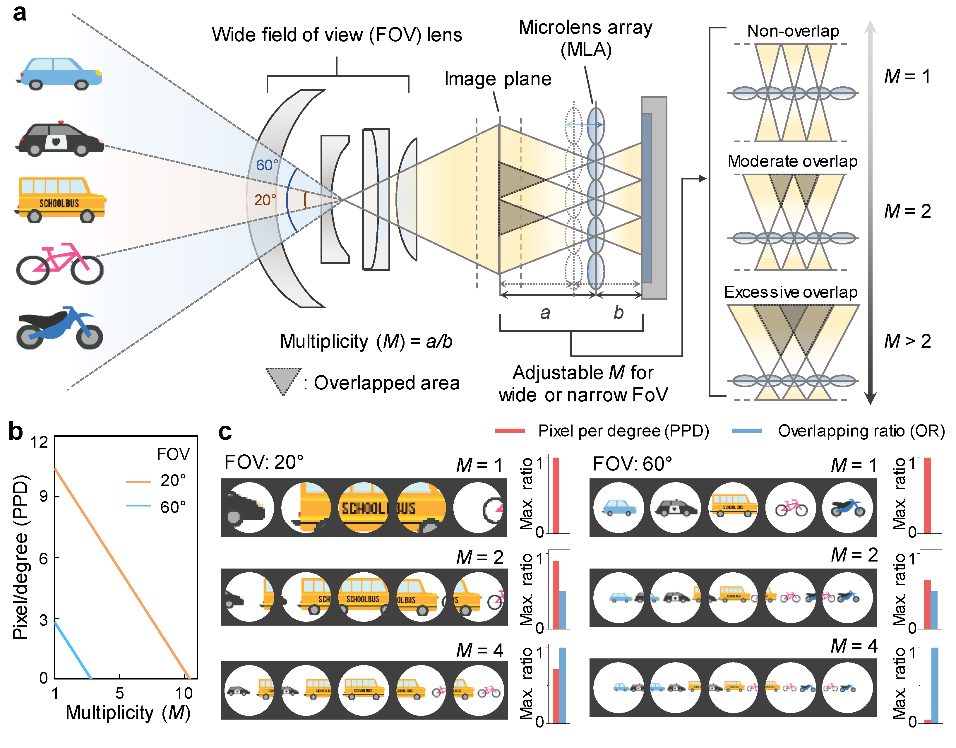
:1. Introduction
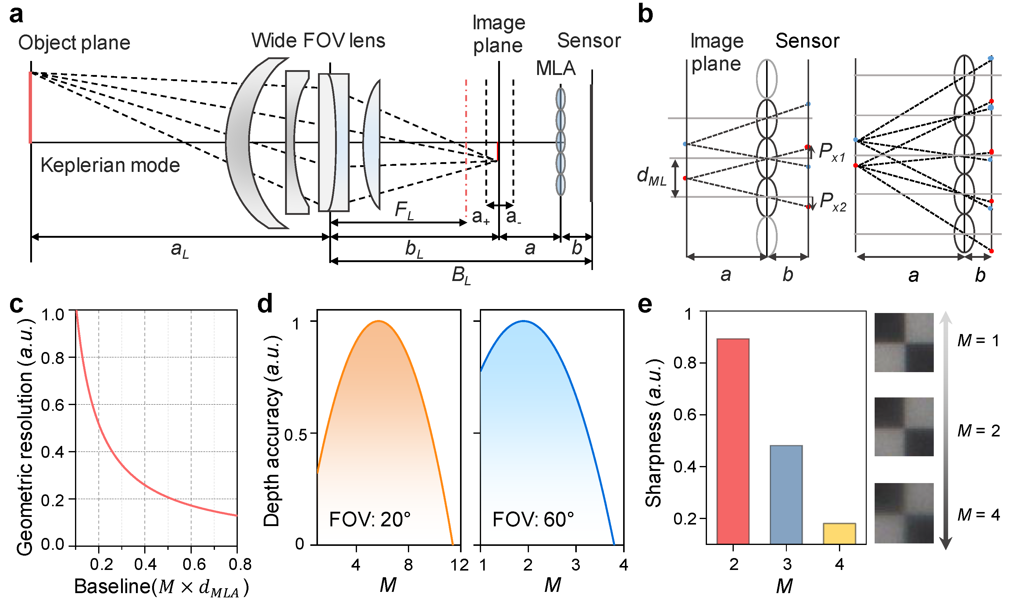
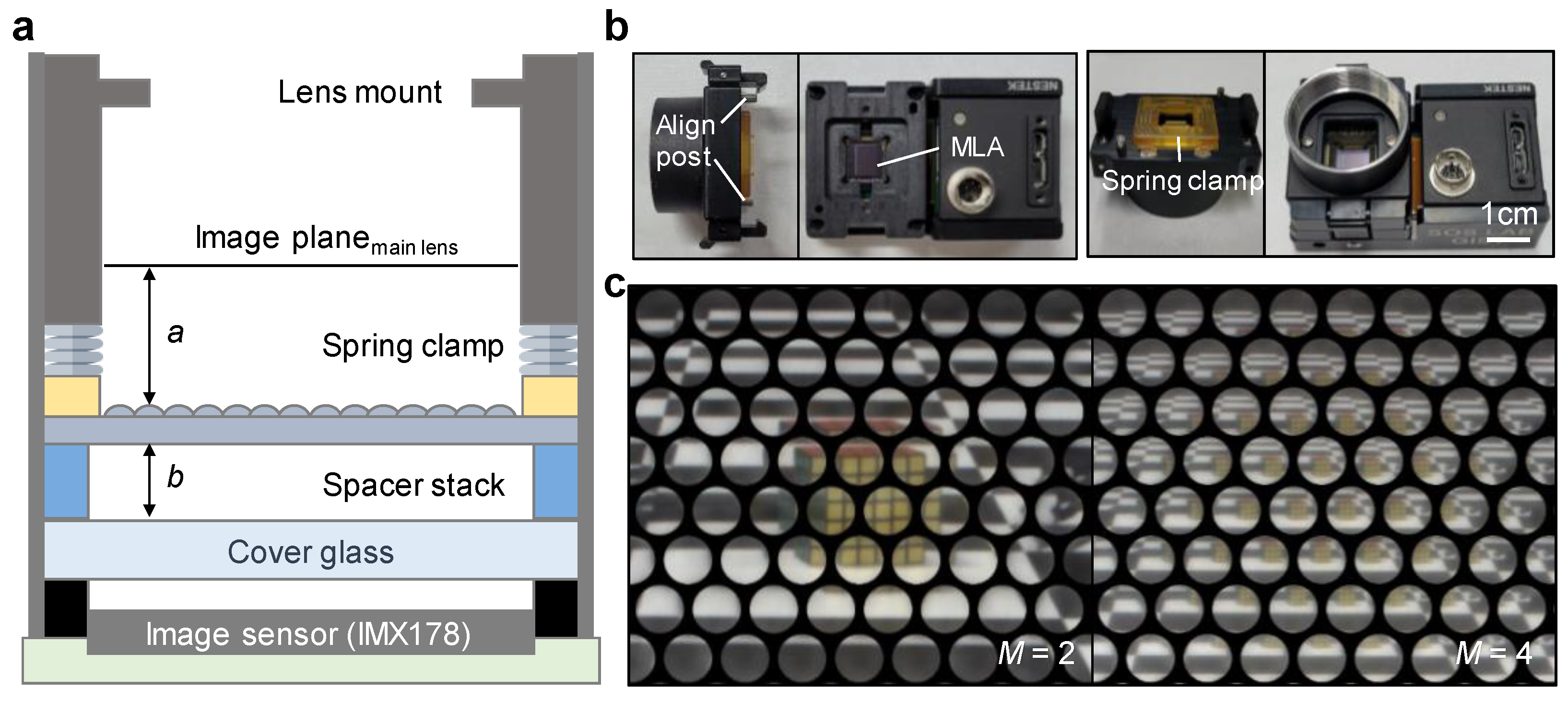
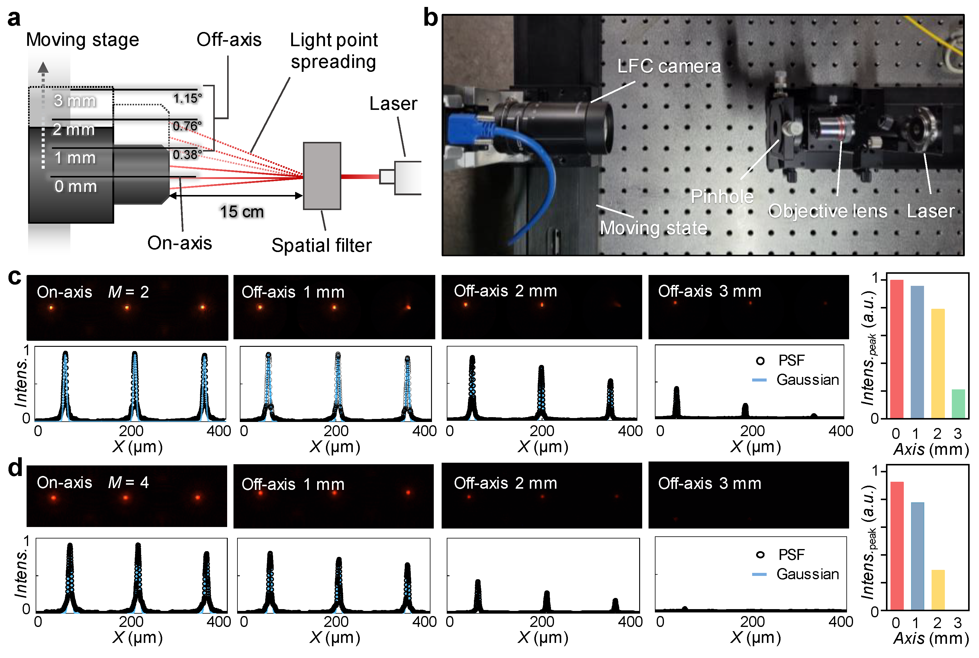
2. Materials and Methods
3. Results and Discussion
4. Conclusions
Author Contributions
Funding
Institutional Review Board Statement
Informed Consent Statement
Conflicts of Interest
References
- Gallwitz, K.L. The Handbook of Italian Renaissance Painters; Prestel: Munich, Germany, 1999. [Google Scholar]
- Thomas, A. The Painter’s Practice in Renaissance Tuscany; Cambridge University Press Cambridge: Cambridge, UK, 1995. [Google Scholar]
- Fraser, H. The Victorians and Renaissance Italy; Blackwell Oxford: Hoboken, NJ, USA, 1992. [Google Scholar]
- Mills, A.A. Vermeer and the camera obscura: Some practical considerations. Leonardo 1998, 31, 213–218. [Google Scholar] [CrossRef]
- Steadman, P. Vermeer and the problem of painting inside the camera obscura. In BAND 2,2 Instrumente des Sehens; De Gruyter: Berlin, Germany, 2004. [Google Scholar]
- Lippmann, G. Epreuves reversibles donnant la sensation du relief. J. Phys. Theor. Appl. 1908, 7, 821–825. [Google Scholar] [CrossRef]
- Adelson, E.H.; Wang, J.Y. Single lens stereo with a plenoptic camera. IEEE Trans. Pattern Anal. Mach. Intell. 1992, 14, 99–106. [Google Scholar] [CrossRef] [Green Version]
- Ng, R.; Levoy, M.; Brédif, M.; Duval, G.; Horowitz, M.; Hanrahan, P. Light Field Photography with a Hand-Held Plenoptic Camera. Ph.D. Thesis, Stanford University, Stanford, CA, USA, 2005. [Google Scholar]
- Georgiev, T.; Lumsdaine, A. Superresolution with plenoptic 2.0 cameras. In Proceedings of the Signal Recovery and Synthesis, San Jose, CA, USA, 13–14 October 2009; p. STuA6. [Google Scholar]
- Georgiev, T.G.; Lumsdaine, A. Depth of Field in Plenoptic Cameras. In Proceedings of the Eurographics (Short Papers), New Orleans, LA, USA, 1–2 August 2009; pp. 5–8. [Google Scholar]
- Georgiev, T.G.; Lumsdaine, A. Focused plenoptic camera and rendering. J. Electron. Imaging 2010, 19, 021106. [Google Scholar]
- Lumsdaine, A.; Georgiev, T. The focused plenoptic camera. In Proceedings of the 2009 IEEE International Conference on Computational Photography, San Francisco, CA, USA, 16–17 April 2009; pp. 1–8. [Google Scholar]
- Dansereau, D.G.; Williams, S.B.; Corke, P.I. Simple change detection from mobile light field cameras. Comput. Vis. Image Underst. 2016, 145, 160–171. [Google Scholar] [CrossRef]
- Dong, F.; Ieng, S.-H.; Savatier, X.; Etienne-Cummings, R.; Benosman, R. Plenoptic cameras in real-time robotics. Int. J. Robot. Res. 2013, 32, 206–217. [Google Scholar] [CrossRef]
- Edussooriya, C.U.; Bruton, L.T.; Agathoklis, P. Enhancing moving objects in light field videos using 5-D IIR adaptive depth-velocity filters. In Proceedings of the 2015 IEEE Pacific Rim Conference on Communications, Computers and Signal Processing, Victoria, BC, Canada, 24–26 August 2015; pp. 169–173. [Google Scholar]
- Shademan, A.; Decker, R.S.; Opfermann, J.; Leonard, S.; Kim, P.C.; Krieger, A. Plenoptic cameras in surgical robotics: Calibration, registration, and evaluation. In Proceedings of the 2016 IEEE International Conference on Robotics and Automation, Stockholm, Sweden, 16–21 May 2016; pp. 708–714. [Google Scholar]
- Skinner, K.A.; Johnson-Roberson, M. Towards real-time underwater 3D reconstruction with plenoptic cameras. In Proceedings of the 2016 IEEE/RSJ International Conference on Intelligent Robots and Systems, Daejeon, Korea, 9–14 October 2016; pp. 2014–2021. [Google Scholar]
- Gandhi, T.; Trivedi, M.M. Vehicle mounted wide FOV stereo for traffic and pedestrian detection. In Proceedings of the IEEE International Conference on Image Processing, Genoa, Italy, 11–14 September 2005; p. II-121. [Google Scholar]
- Scaramuzza, D.; Siegwart, R. Appearance-guided monocular omnidirectional visual odometry for outdoor ground vehicles. IEEE Trans. Robot. 2008, 24, 1015–1026. [Google Scholar] [CrossRef] [Green Version]
- Birklbauer, C.; Bimber, O. Panorama Light-Field Imaging. In Proceedings of the Graphics Forum. 2014, pp. 43–52. Available online: https://onlinelibrary.wiley.com/doi/abs/10.1111/cgf.12289 (accessed on 20 March 2022).
- Guo, X.; Yu, Z.; Kang, S.B.; Lin, H.; Yu, J. Enhancing light fields through ray-space stitching. IEEE Trans. Vis. Comput. Graph. 2015, 22, 1852–1861. [Google Scholar] [CrossRef] [PubMed]
- Dansereau, D.G.; Schuster, G.; Ford, J.; Wetzstein, G. A wide-field-of-view monocentric light field camera. In Proceedings of the IEEE Conference on Computer Vision and Pattern Recognition, Honolulu, HI, USA, 21–26 July 2017; pp. 5048–5057. [Google Scholar]
- Schuster, G.M.; Dansereau, D.G.; Wetzstein, G.; Ford, J.E. Panoramic single-aperture multi-sensor light field camera. Opt. Express 2019, 27, 37257–37273. [Google Scholar] [CrossRef] [PubMed]
- Bhavsar, A.V.; Rajagopalan, A. Resolution enhancement for binocular stereo. In Proceedings of the 2008 19th International Conference on Pattern Recognition, Tampa, FL, USA, 8–11 December 2008; pp. 1–4. [Google Scholar]
- Bishop, T.E.; Favaro, P. The light field camera: Extended depth of field, aliasing, and superresolution. IEEE Trans. Pattern Anal. Mach. Intell. 2011, 34, 972–986. [Google Scholar] [CrossRef] [PubMed]
- Reulke, R.; Säuberlich, T. Image quality of optical remote sensing data. In Proceedings of the Electro-Optical Remote Sensing, Photonic Technologies, and Applications VIII, and Military Applications in Hyperspectral Imaging and High Spatial Resolution Sensing II, Amsterdam, The Netherlands, 22 September 2014; pp. 132–140. [Google Scholar]
- Kim, H.M.; Kim, M.S.; Chang, S.; Jeong, J.; Jeon, H.-G.; Song, Y.M. Vari-Focal Light Field Camera for Extended Depth of Field. Micromachines 2021, 12, 1453. [Google Scholar] [CrossRef] [PubMed]
- Zeller, N.; Quint, F.; Stilla, U. Calibration and accuracy analysis of a focused plenoptic camera. ISPRS Ann. Photogramm. Remote Sens. Spat. Inf. Sci. 2014, 2, 205. [Google Scholar] [CrossRef] [Green Version]
- Gallup, D.; Frahm, J.-M.; Mordohai, P.; Pollefeys, M. Variable baseline/resolution stereo. In Proceedings of the 2008 IEEE Conference on Computer Vision and Pattern Recognition, Anchorage, AK, USA, 23–28 June 2008; pp. 1–8. [Google Scholar]
- Janout, P.; Páta, P.; Skala, P.; Bednář, J. PSF Estimation of Space-Variant Ultra-Wide Field of View Imaging Systems. Appl. Sci. 2017, 7, 151. [Google Scholar] [CrossRef] [Green Version]
- Trouve, P.; Champagnat, F.; Besnerais, G.; Druart, G.; Idier, J. Design of a chromatic 3D camera with an end-to-end performance model approach. In Proceedings of the IEEE Conference on Computer Vision and Pattern Recognition Workshops, Washington, DC, USA, 23–28 June 2013; pp. 953–960. [Google Scholar]
- Niskanen, M.; Silvén, O.; Tico, M. Video stabilization performance assessment. In Proceedings of the 2006 IEEE International Conference on Multimedia and Expo, Toronto, ON, USA, 9–12 July 2006; pp. 405–408. [Google Scholar]
- Palmieri, L.; Koch, R.; Veld, R.O.H. The Plenoptic 2.0 Toolbox: Benchmarking of Depth Estimation Methods for MLA-Based Focused Plenoptic Cameras. In Proceedings of the 2018 25th IEEE International Conference on Image Processing, Athens, Greece, 7–10 October 2018; pp. 649–653. [Google Scholar]
- Zhou, P.; Cai, W.; Yu, Y.; Zhang, Y.; Zhou, G. A two-step calibration method of lenslet-based light field cameras. Opt. Lasers Eng. 2019, 115, 190–196. [Google Scholar] [CrossRef]
- Conti, C.; Soares, L.D.; Nunes, P. Dense light field coding: A survey. IEEE Access 2020, 8, 49244–49284. [Google Scholar] [CrossRef]
- Taguchi, Y.; Agrawal, A.; Ramalingam, S.; Veeraraghavan, A. Axial light field for curved mirrors: Reflect your perspective, widen your view. In Proceedings of the 2010 IEEE Computer Society Conference on Computer Vision and Pattern Recognition, San Francisco, CA, USA, 13–18 June 2010; pp. 499–506. [Google Scholar]
- Popovic, V.; Afshari, H.; Schmid, A.; Leblebici, Y. Real-time implementation of Gaussian image blending in a spherical light field camera. In Proceedings of the 2013 IEEE International Conference on Industrial Technology, Cape Town, South Africa, 25–28 February 2013; pp. 1173–1178. [Google Scholar]
- Akin, A.; Cogal, O.; Seyid, K.; Afshari, H.; Schmid, A.; Leblebici, Y. Hemispherical multiple camera system for high resolution omni-directional light field imaging. IEEE J. Emerg. Sel. Top. Circuits Syst. 2013, 3, 137–144. [Google Scholar] [CrossRef]


| Technique | Lens | Additional Components | Num. of Image Sensors | Image Acquisition (Frames) | Field-of-View (FOV per Frame) | Ref |
|---|---|---|---|---|---|---|
| Panoramic single aperture | Monocentric lens | Relay optics, Horizontal rotating stage | 1 | Sequential capture (11) | 138° (24°) | [23] |
| Panoramic monocentric | Monocentric lens | Multiple consolidators, Multiple fiber bundles | 5 | Multiple capture (5) | 140° (32°) | [20] |
| Axial light field | Conventional lens | Spherical mirror, Rotating stage | 1 | Sequential capture (25) | 140° (32°) | [36] |
| Gaussian image blending | Multiple conventional lenses | Hemispherical support, FPGA board | 15 | Multiple capture (15) | 360° (36°) | [37] |
| Omni-directional light-field imaging | Multiple conventional lenses | Hemispherical support, FPGA board | 44 | Multiple capture (44) | 360° (53°) | [38] |
| Adjustable multiplicity | Conventional lens | Adjustable spacer | 1 | Single capture | 60° | This work |
Publisher’s Note: MDPI stays neutral with regard to jurisdictional claims in published maps and institutional affiliations. |
© 2022 by the authors. Licensee MDPI, Basel, Switzerland. This article is an open access article distributed under the terms and conditions of the Creative Commons Attribution (CC BY) license (https://creativecommons.org/licenses/by/4.0/).
Share and Cite
Kim, H.M.; Yoo, Y.J.; Lee, J.M.; Song, Y.M. A Wide Field-of-View Light-Field Camera with Adjustable Multiplicity for Practical Applications. Sensors 2022, 22, 3455. https://doi.org/10.3390/s22093455
Kim HM, Yoo YJ, Lee JM, Song YM. A Wide Field-of-View Light-Field Camera with Adjustable Multiplicity for Practical Applications. Sensors. 2022; 22(9):3455. https://doi.org/10.3390/s22093455
Chicago/Turabian StyleKim, Hyun Myung, Young Jin Yoo, Jeong Min Lee, and Young Min Song. 2022. "A Wide Field-of-View Light-Field Camera with Adjustable Multiplicity for Practical Applications" Sensors 22, no. 9: 3455. https://doi.org/10.3390/s22093455
APA StyleKim, H. M., Yoo, Y. J., Lee, J. M., & Song, Y. M. (2022). A Wide Field-of-View Light-Field Camera with Adjustable Multiplicity for Practical Applications. Sensors, 22(9), 3455. https://doi.org/10.3390/s22093455