
Real-Time Adaptive Modulation Schemes for Underwater Acoustic OFDM Communication


Abstract
:1. Introduction
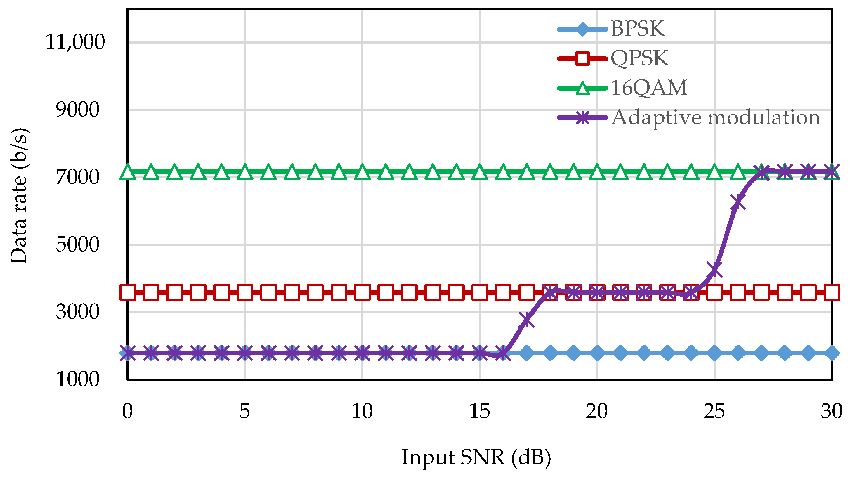
- To choose a proper modulation, depending on the channel conditions, to improve the system throughput under a fixed bit error rate (BER).
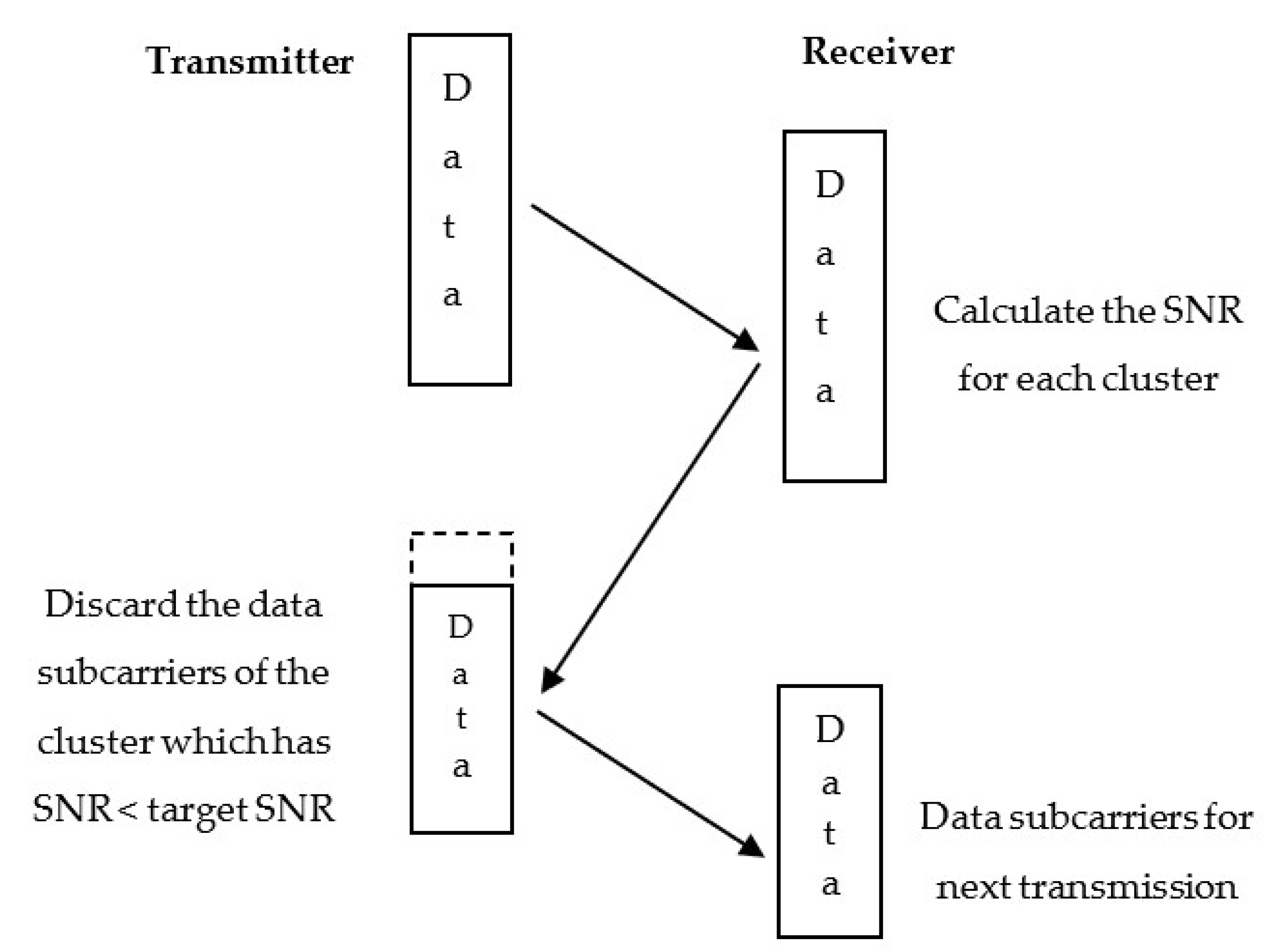
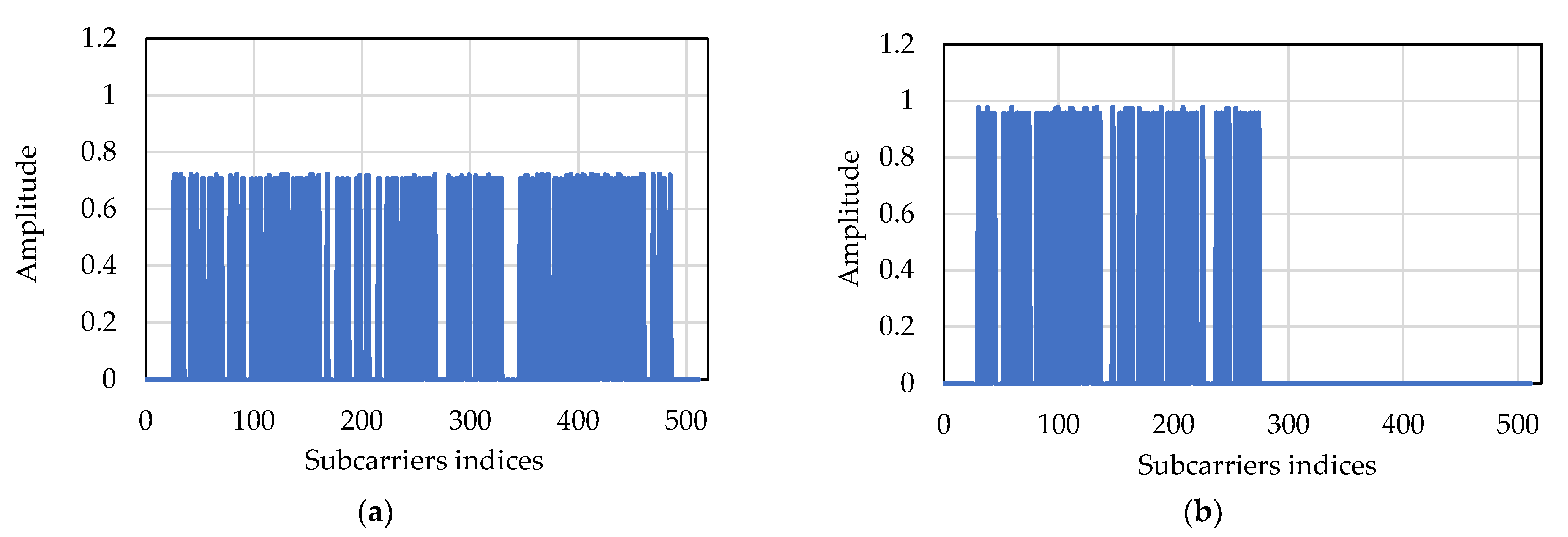
- To discard subcarriers that experience deep fade to improve the energy efficiency of the system. Discarding the deep-faded (weak) subcarriers helps to save the energy which is wasted to transmit the deep-faded subcarriers, and this energy is distributed on the remaining subcarriers for the next transmission.
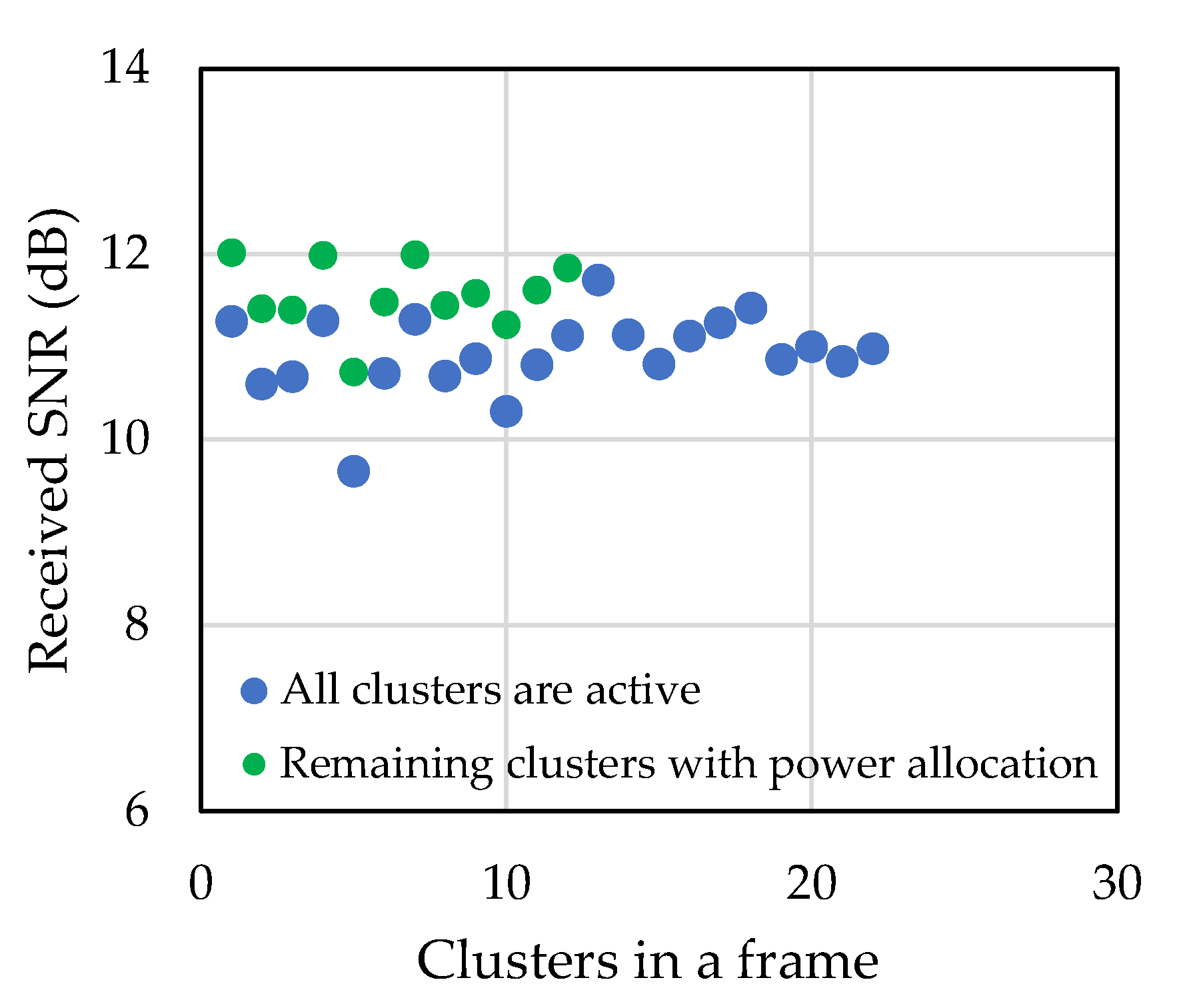
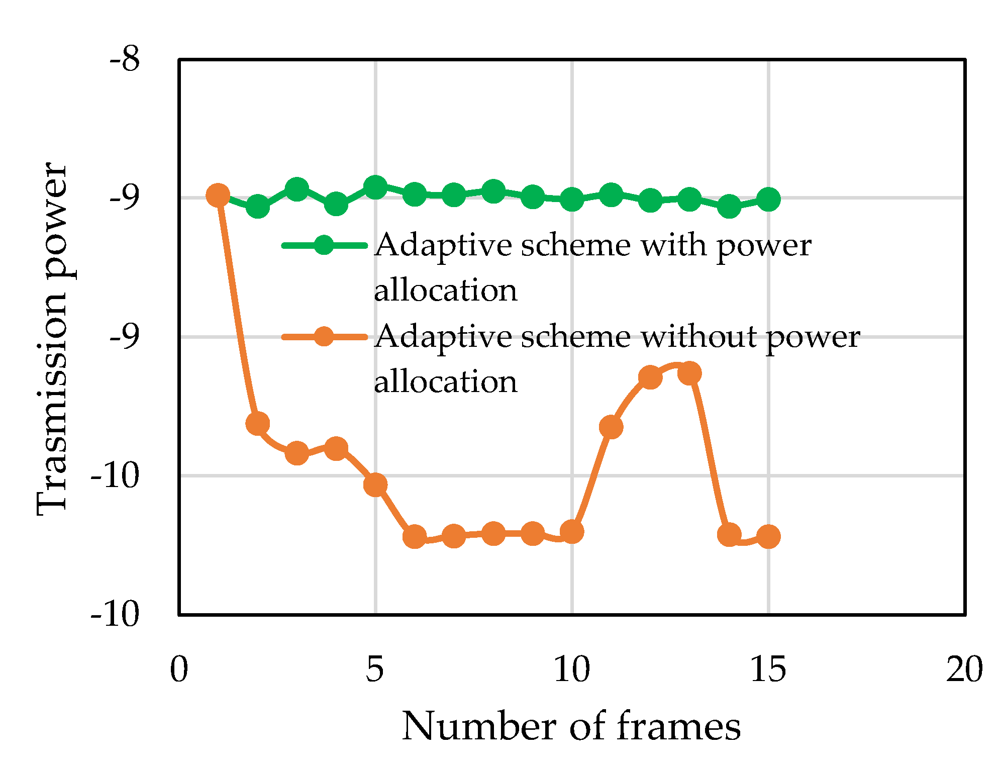
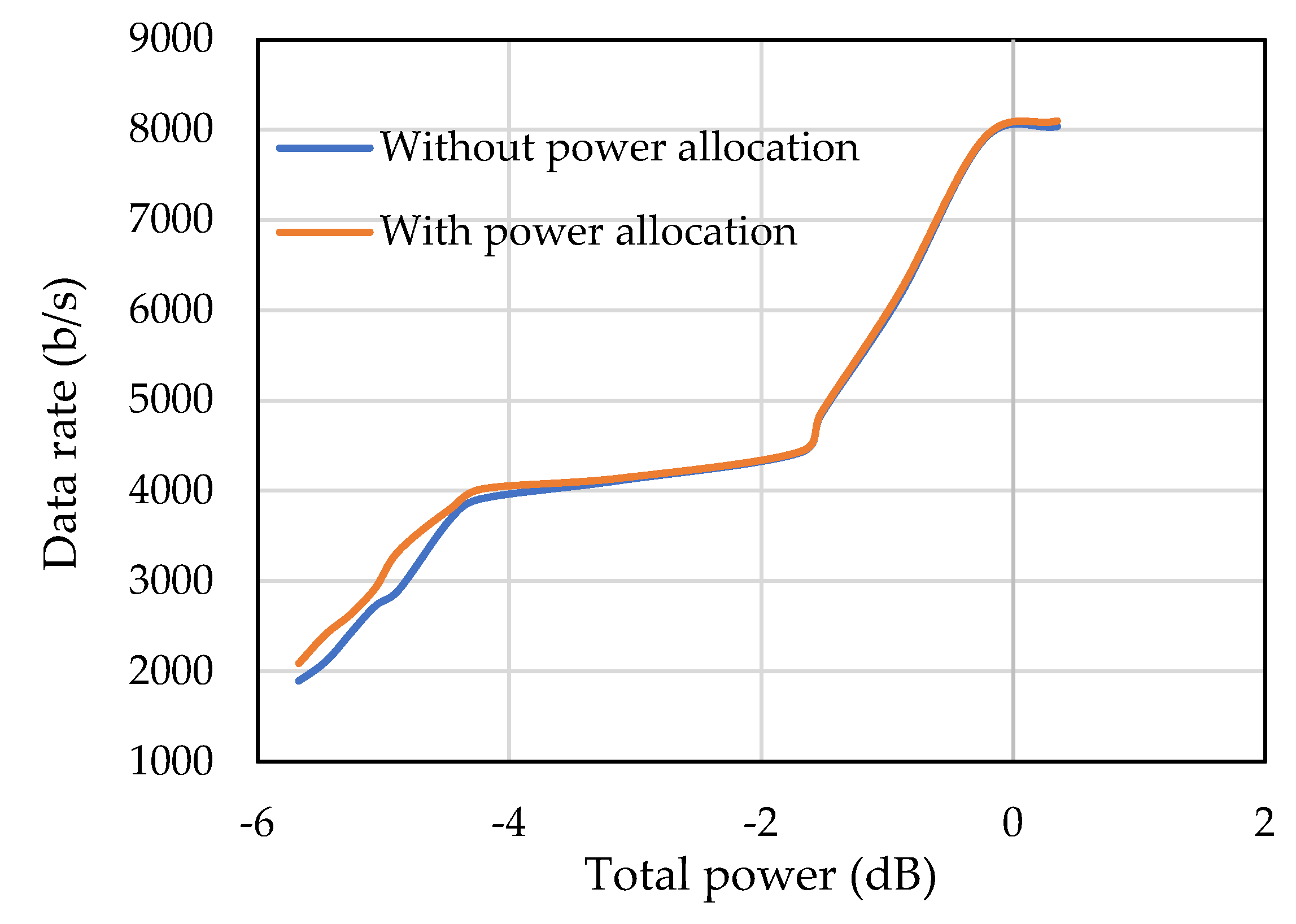
- To distribute the residual power among the remaining subcarriers, which ensures constant transmitted symbol energy, despite the channel variation, to achieve overall better throughput of the system.
2. Background
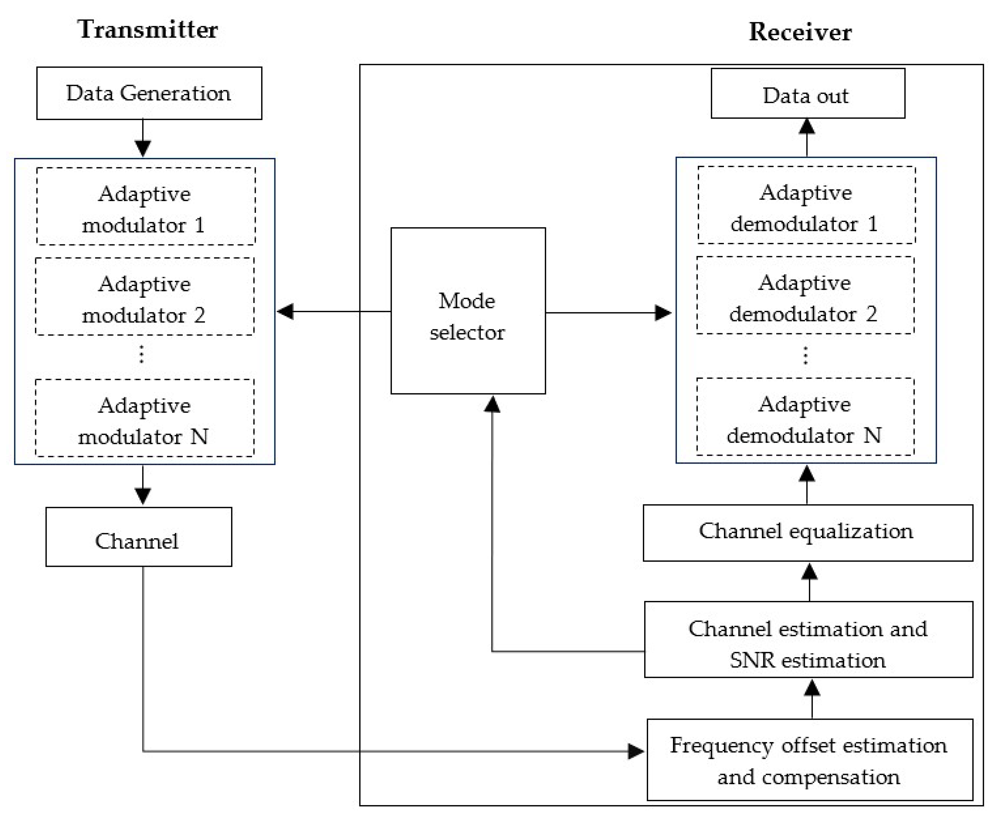
3. System Model
- Pilot subcarriers are used for channel estimation.
- Data subcarriers are used to carry information symbols.
- Null subcarriers are used at the edge of the frequency band to prevent spectrum leakage. Null subcarriers are also placed among the active subcarriers (pilot and data subcarriers) to facilitate Doppler estimation and noise variance estimation.
3.1. CFO Estimation
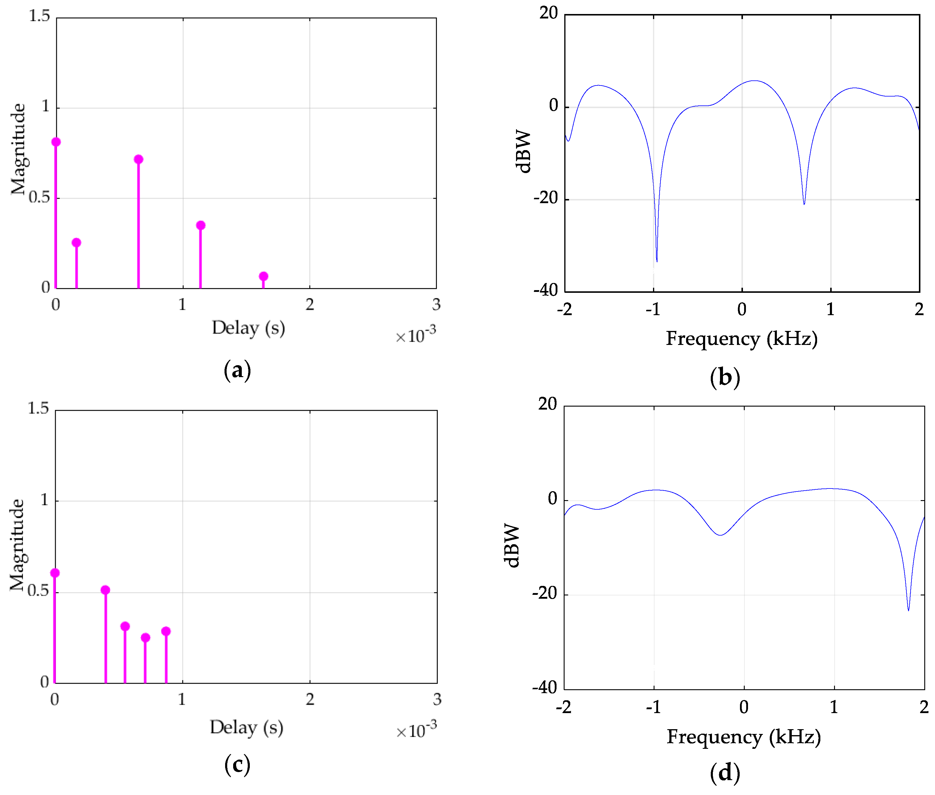
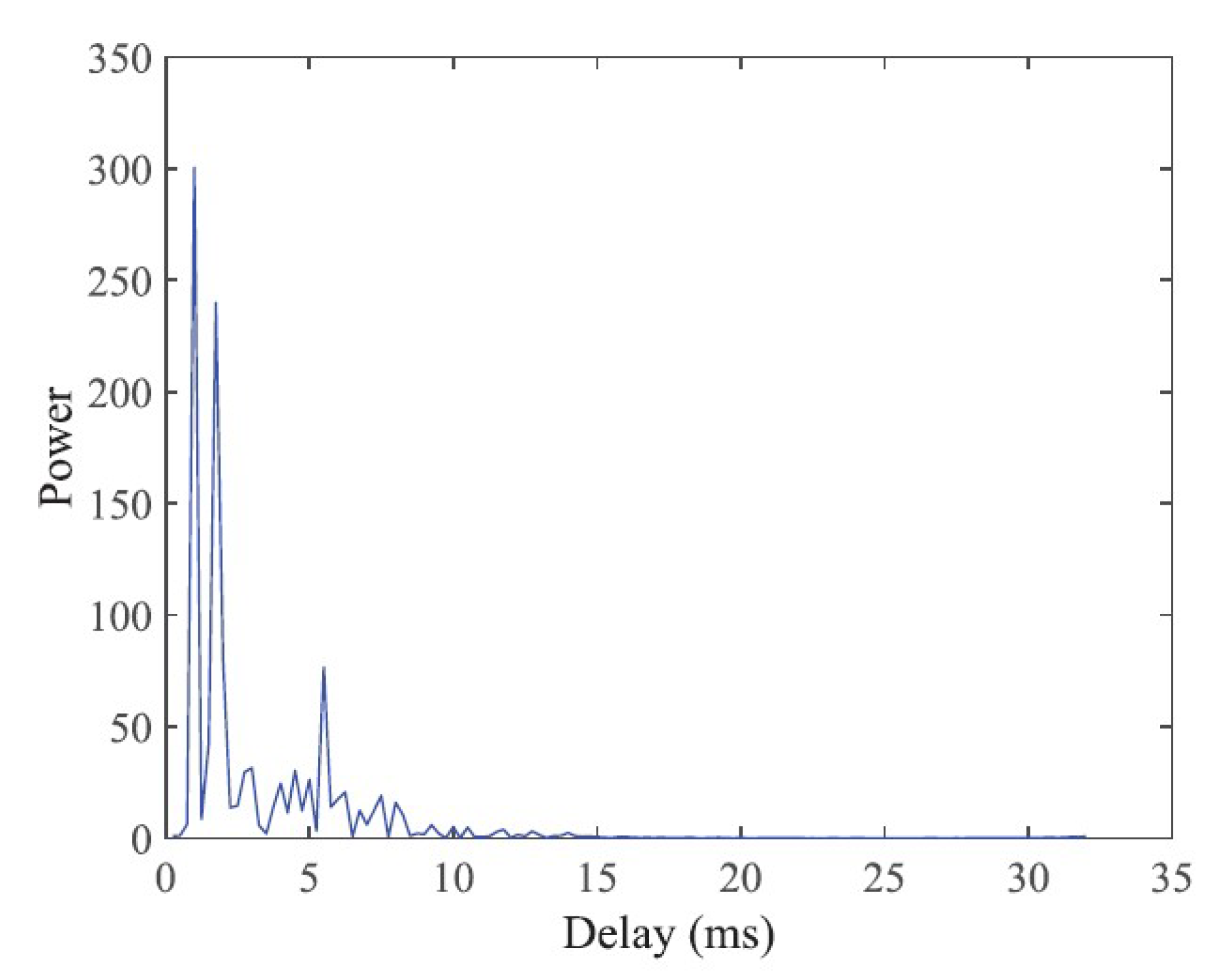
3.2. Channel Estimation
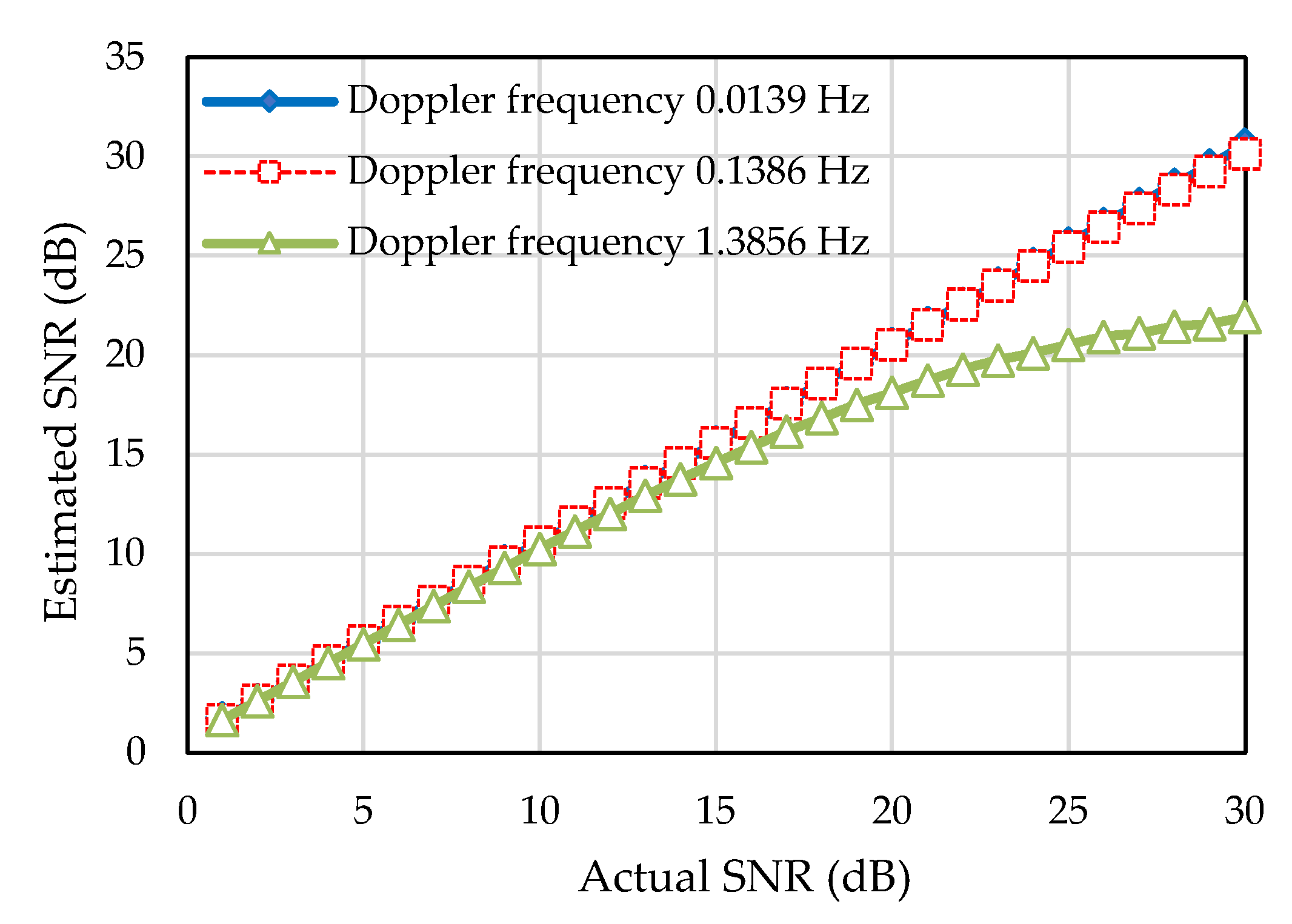
3.3. SNR Estimation
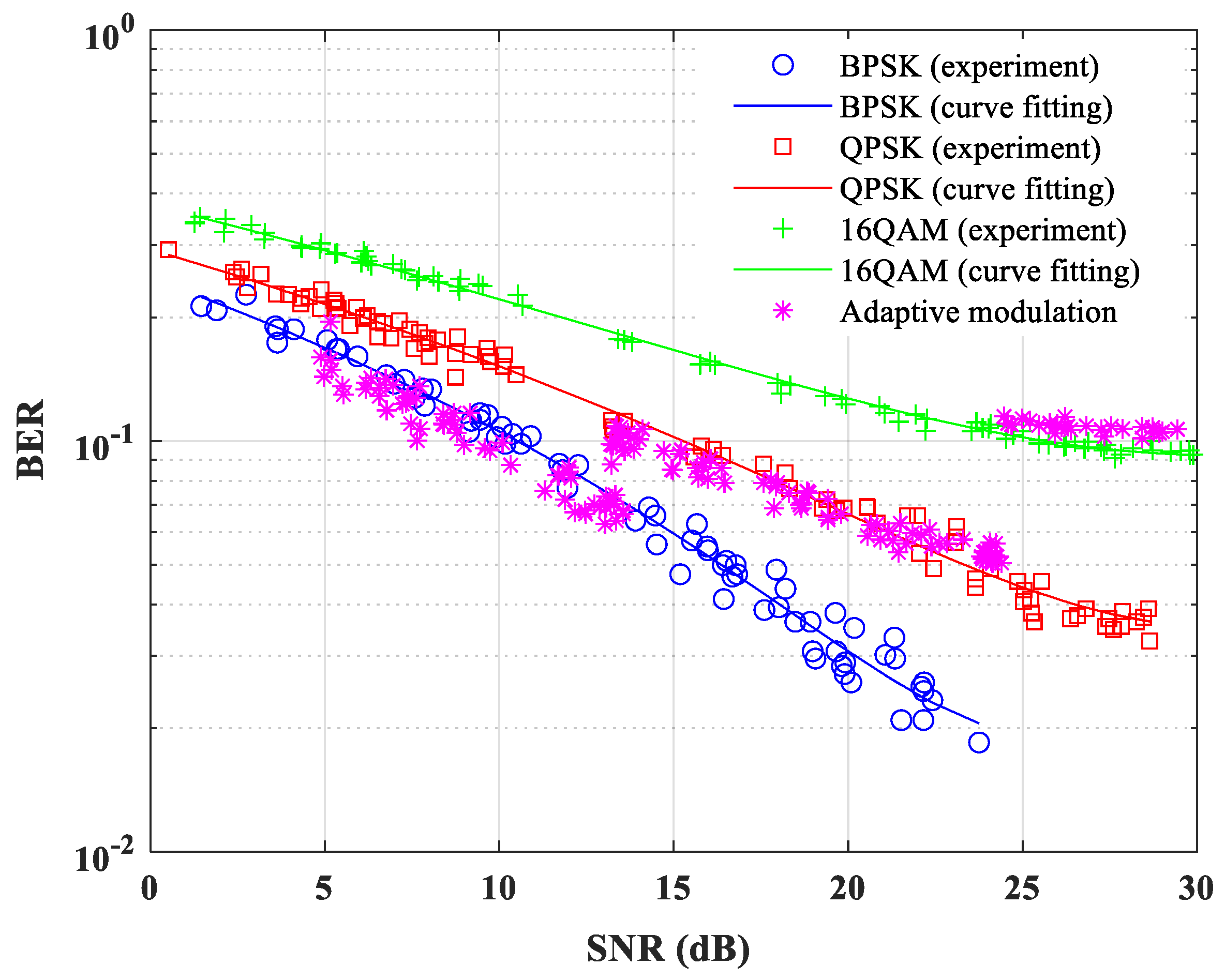
4. Adaptive Modulation
4.1. Frame-Based Adaptive Modulation
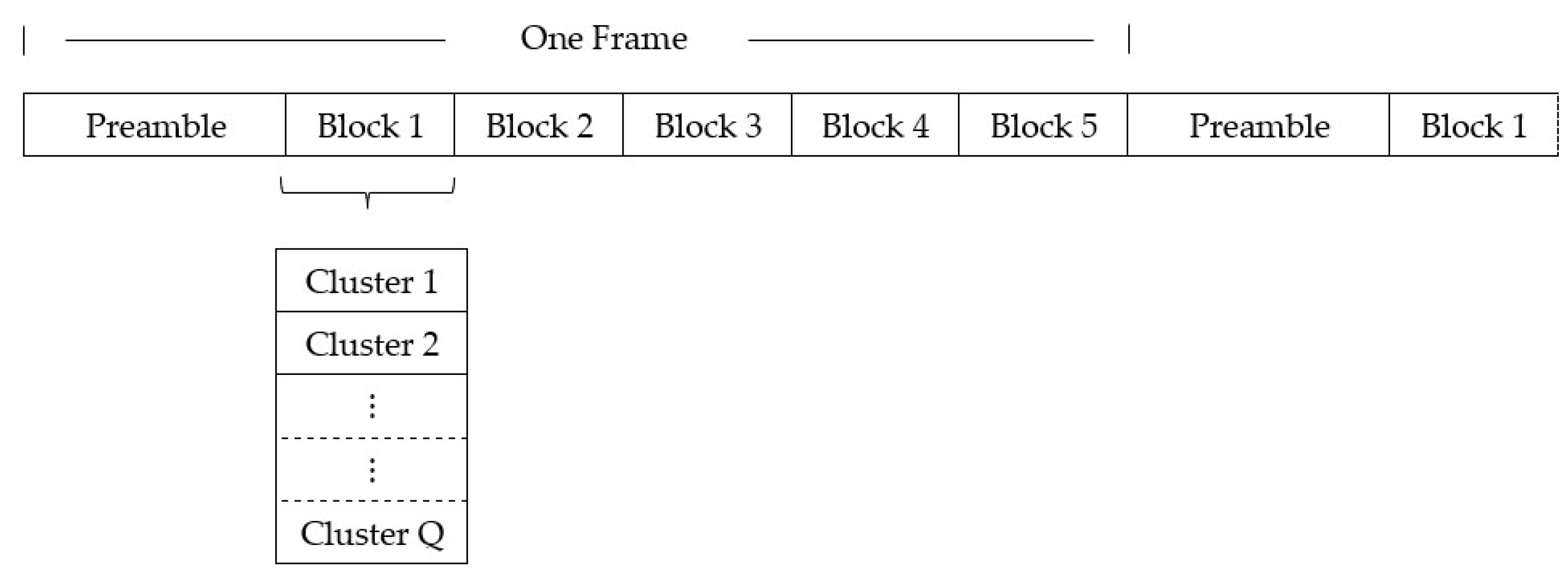
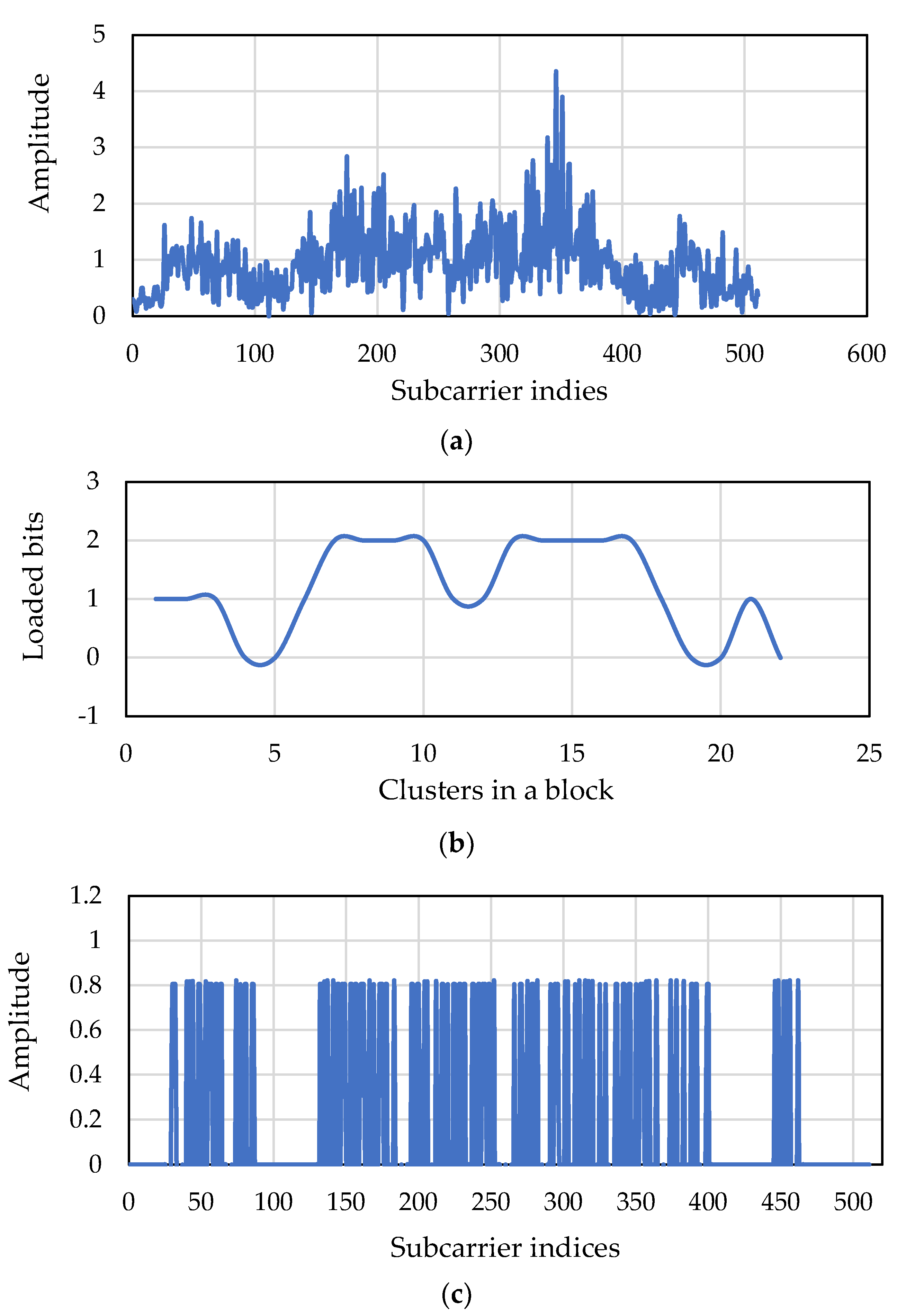
4.2. Cluster-Based Adaptive Modulation
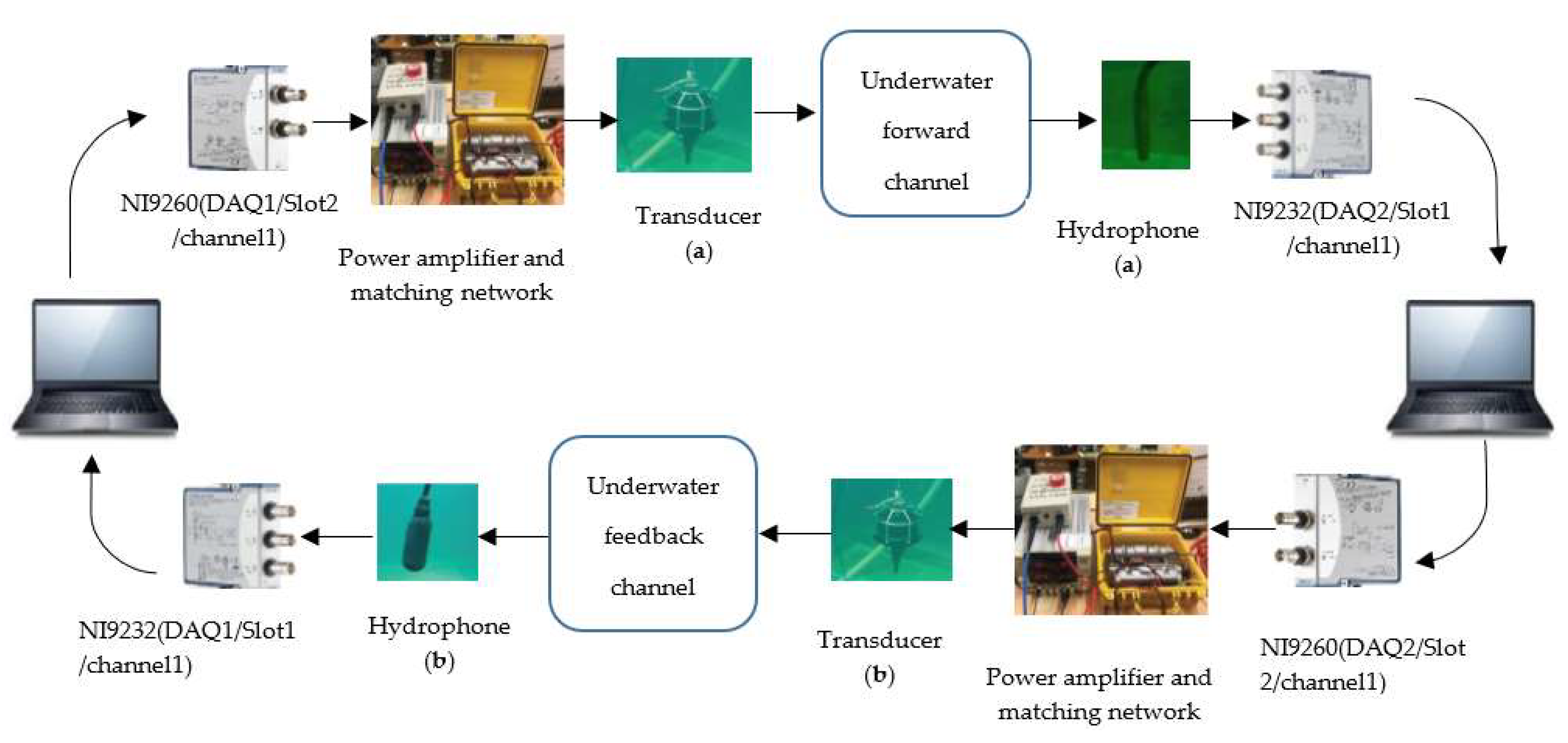
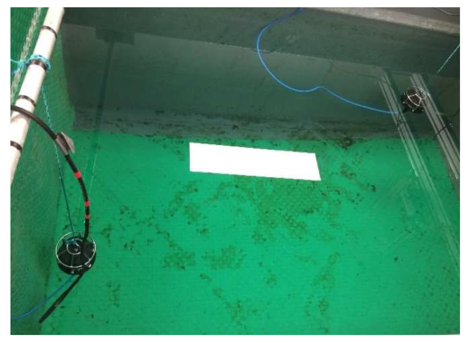
5. System Implementation
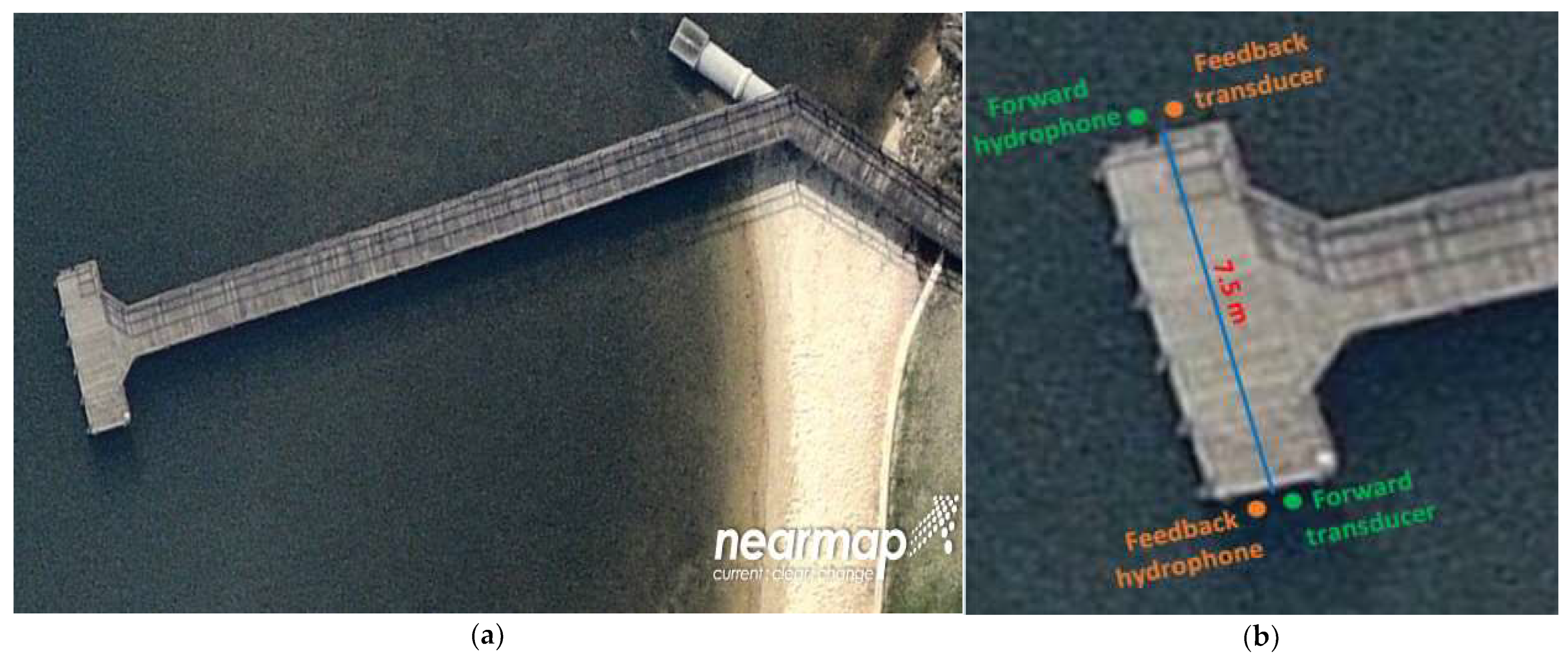
5.1. System Hardware
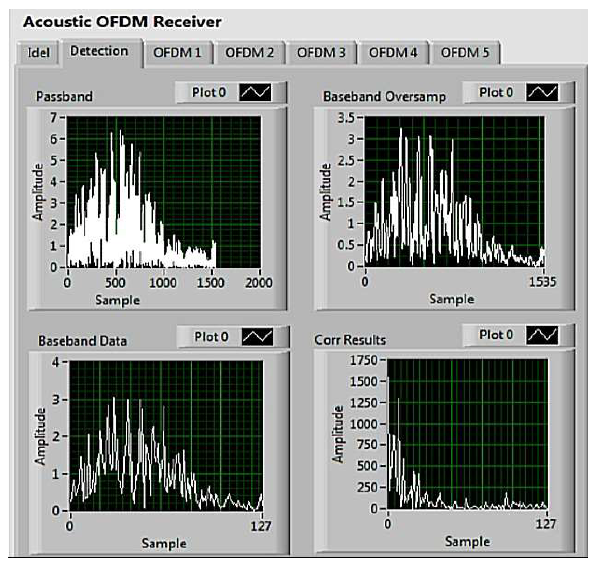
5.2. Software Implementation
6. Results and Discussion
6.1. Frame-Based Adaptive Modulation
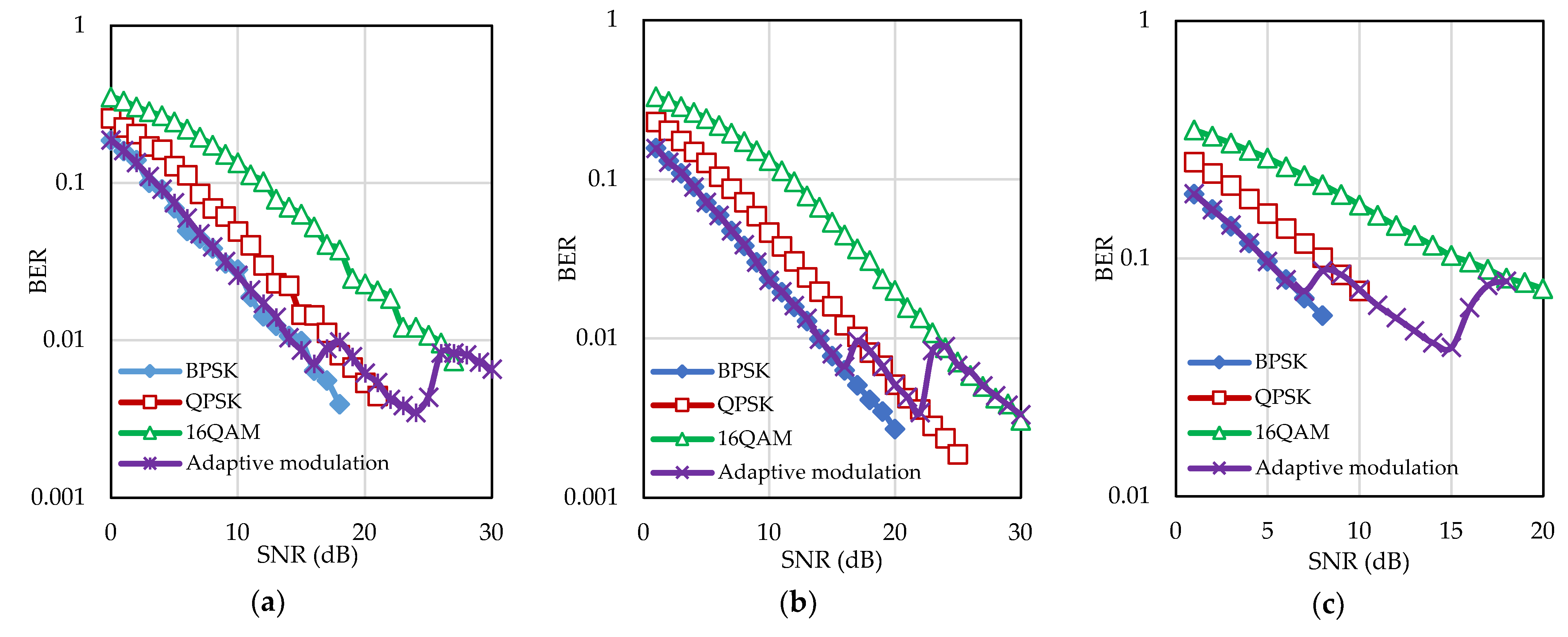
6.1.1. Simulation Results
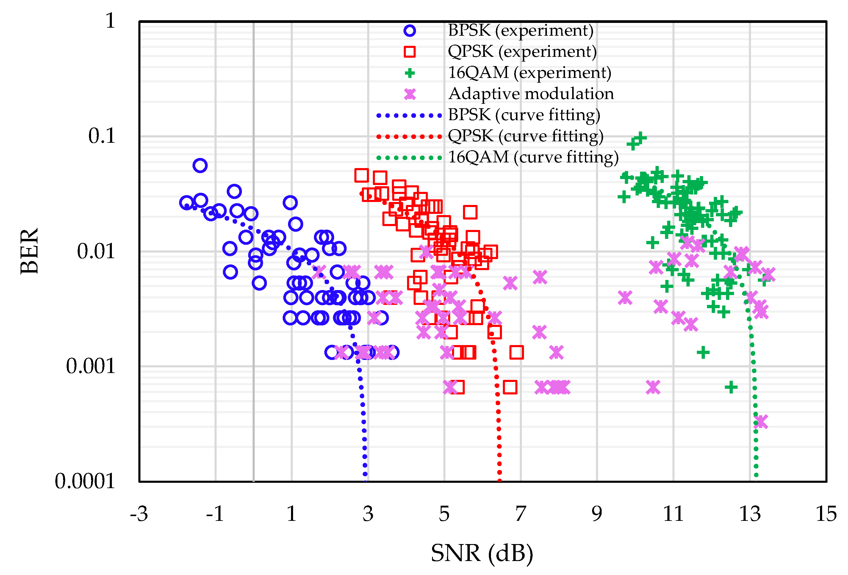
6.1.2. Experimental Results
6.2. Cluster-Based Adaptive Modulation
6.2.1. Experimental Results
7. Conclusions
Author Contributions
Funding
Acknowledgments
Conflicts of Interest
References
- Melodia, T.; Kulhandjian, H.; Kuo, L.C.; Demirors, E. Advances in underwater acoustic networking. In Mobile Ad Hoc NetWorking: Cutting Edge Directions, 2nd ed.; Wiley: Hoboken, NJ, USA, 2013; pp. 804–852. [Google Scholar]
- Ali, M.F.; Jayakody, D.N.K.; Chursin, Y.A.; Affes, S.; Dmitry, S. Recent advances and future directions on underwater wireless communications. Arch. Comput. Methods Eng. 2019, 27, 1379–1412. [Google Scholar] [CrossRef]
- Akyildiz, I.F.; Pompili, D.; Melodia, T. Underwater acoustic sensor networks: Research challenges. Elsevier Ad Hoc Netw. 2005, 3, 257–279. [Google Scholar] [CrossRef]
- Kilfoyle, D.B.; Baggeroer, A.B. The state of the art in underwater acoustic telemetry. IEEE J. Ocean. Eng. 2000, 25, 4–27. [Google Scholar] [CrossRef]
- Zhou, S.; Wang, Z. OFDM for Underwater Acoustic Communications; John Wiley & Sons Ltd.: Hoboken, NJ, USA, 2014. [Google Scholar]
- Chen, P.; Rong, Y.; Nordholm, S.; He, Z.; Duncan, A. Joint channel estimation and impulsive noise mitigation in underwater acoustic OFDM communication systems. IEEE Trans. Wirel. Commun. 2017, 16, 6165–6178. [Google Scholar] [CrossRef]
- Chen, P.; Rong, Y.; Nordholm, S.; He, Z. Joint channel and impulsive noise estimation in underwater acoustic OFDM systems. IEEE Trans. Veh. Technol. 2017, 66, 10567–10571. [Google Scholar] [CrossRef]
- Wan, L.; Zhou, H.; Xu, X.; Huang, Y.; Zhou, S.; Shi, Z.; Cui, J.H. Adaptive modulation and coding for underwater acoustic OFDM. IEEE J. Ocean. Eng. 2015, 40, 327–336. [Google Scholar] [CrossRef]
- Radosevic, A.; Ahmed, R.; Duman, T.M.; Proakis, J.G.; Stojanovic, M. Adaptive OFDM modulation for underwater acoustic communication: Design considerations and experimental results. IEEE J. Ocean. Eng. 2014, 39, 357–370. [Google Scholar] [CrossRef]
- Sadeghi, M.; Elamassie, M.; Uysal, M. Adaptive OFDM-based acoustic underwater transmission: System design and experimental verification. In Proceedings of the IEEE International Black Sea Conference on Communications and Networking, Istanbul, Turkey, 5–8 June 2017; pp. 1–5. [Google Scholar]
- Barua, S.; Rong, Y.; Nordholm, S.; Chen, P. Adaptive modulation for underwater acoustic OFDM communication. In Proceedings of the MTS/IEEE OCEANS, Marseille, France, 17–20 June 2019. [Google Scholar]
- Barua, S.; Rong, Y.; Nordholm, S.; Chen, P. A LabVIEW-based implementation of real-time adaptive modulation for underwater acoustic OFDM communication. In Proceedings of the MTS/IEEE OCEANS, Singapore, 6–9 April 2020. [Google Scholar]
- Barua, S.; Rong, Y.; Nordholm, S.; Chen, P. Real-time subcarrier cluster-based adaptive modulation for underwater acoustic OFDM communications. In Proceedings of the MTS/IEEE OCEANS, Biloxi, MS, USA, 19–22 October 2020. [Google Scholar]
- Chen, P.; Rong, Y.; Nordholm, S.; Duncan, A.; He, Z. A LabVIEW based implementation of real-time underwater acoustic OFDM system. In Proceedings of the 23rd Asia-Pacific Conference on Communications, Perth, WA, Australia, 11–13 December 2017; pp. 1–5. [Google Scholar]
- Chen, P.; Rong, Y.; Nordholm, S.; He, Z. An underwater acoustic OFDM system based on NI CompactDAQ and LabVIEW. IEEE Syst. J. 2019, 13, 3858–3868. [Google Scholar] [CrossRef]
- Stojanovic, M.; Preisig, J. Underwater acoustic communication channels: Propagation models and statistical characterization. IEEE Commun. Mag. 2009, 47, 84–89. [Google Scholar] [CrossRef]
- Badiey, M.; Mu, Y.; Simmen, J.A.; Forsythe, S.E. Signal variability in shallow-water sound channels. IEEE J. Ocean. Eng. 2000, 25, 492–500. [Google Scholar] [CrossRef]
- Song, A.; Badiey, M.; Song, H.-C.; Hodgkiss, W.S.; Porter, M.B.; KauaiEx Group. Impact of ocean variability on coherent underwater acoustic communications during the Kauai experiment (KauaiEx). J. Acoust. Soc. Am. 2008, 123, 856–865. [Google Scholar] [CrossRef] [PubMed] [Green Version]
- Stojanovic, M. Recent advances in high-speed underwater acoustic communications. IEEE J. Ocean. Eng. 1996, 21, 125–136. [Google Scholar] [CrossRef]
- Chitre, M.; Shahabudeen, S.; Stojanovic, M. Underwater acoustic communications & networking: Recent advances and future challenges. Mar. Technol. Soc. J. 2008, 42, 103–116. [Google Scholar]
- Freitag, L.; Grund, M.; Singh, S.; Partan, J.; Koski, P.; Ball, K. The WHOI Micro-Modem: An acoustic communications and navigation system for multiple platforms. In Proceedings of the OCEANS 2005, Washington, DC, USA, 17–23 September 2005; Volume 2, pp. 1086–1092. [Google Scholar]
- Sozer, E.; Stojanovic, M. Reconfigurable acoustic modem for underwater sensor networks. In Proceedings of the 1st ACM International Workshop on UnderWater Networks (WUWNet), Los Angeles, CA, USA, 25 September 2006; pp. 101–104. [Google Scholar]
- Tong, F.; Zhou, S.; Benson, B.; Kastner, R. R & D of dual mode acoustic modem test bed for shallow water channels. In Proceedings of the ACM International Workshop on UnderWater Networks (WUWNet), Woods Hole, MA, USA, 30 September 2010; pp. 1–4. [Google Scholar]
- Yan, H.; Wan, L.; Zhou, S.; Shi, Z.; Cui, J.-H.; Huang, J.; Zhou, H. DSP based receiver implementation for OFDM acoustic modems. Elsevier J. Phys. Commun. 2012, 5, 22–32. [Google Scholar] [CrossRef]
- Yan, H.; Zhou, S.; Shi, Z.; Li, B. A DSP implementation of OFDM acoustic modem. In Proceedings of the ACM International Workshop on UnderWater Networks (WUWNet), Montréal, Qc, Canada, 14 September 2007. [Google Scholar]
- Shen, X.; Wang, H.; Zhang, Y.; Zhao, R. Adaptive Technique for Underwater Acoustic Communication; InTech: Yokohama, Japan, 2012. [Google Scholar]
- Pelekanakis, K.; Cazzanti, L.; Zappa, G. Decision tree-based adaptive modulation for underwater acoustic communications. In Proceedings of the IEEE OES Third Underwater Communications and Networking Conference, Lerici, Italy, 30 August–1 September 2016; pp. 1–5. [Google Scholar]
- Wan, L. Underwater Acoustic OFDM: Algorithm Design, DSP Implementation, and Field Performance. Ph.D. Thesis, University of Connecticut, Connecticut, CT, USA, 2014. [Google Scholar]
- Dol, H.S.; Casari, P.; van der Zwan, T.; Otnes, R. Software-defined underwater acoustic modems: Historical review and the NILUS approach. IEEE J. Ocean. Eng. 2017, 42, 722–737. [Google Scholar] [CrossRef]
- Radosevic, A.; Duman, T.M.; Proakis, J.G.; Stojanovic, M. Channel prediction for adaptive modulation in underwater acoustic communications. In Proceedings of the OCEANS 2011, Santander, Spain, 6–9 June 2011; pp. 1–5. [Google Scholar]
- Stojanovic, M. OFDM for underwater acoustic communications: Adaptive synchronization and sparse channel estimation. In Proceedings of the IEEE International Conference on Acoustics, Speech and Signal Processing, Las Vegas, NV, USA, 31 March–4 April 2008; pp. 5288–5291. [Google Scholar]
- Tureli, U.; Liu, H.; Zoltowski, M.D. OFDM blind carrier offset estimation: ESPRIT. IEEE Trans. Commun. 2000, 48, 1459–1461. [Google Scholar] [CrossRef]
- Li, B.; Zhou, S.; Stojanovic, M.; Freitag, L.; Willett, P. Multicarrier communication over underwater acoustic channels with nonuniform Doppler shifts. IEEE J. Ocean. Eng. 2008, 33, 198–209. [Google Scholar]
- Huang, M.; Sun, S.; Cheng, E.; Kuai, X.; Xu, X. Joint interference mitigation with channel estimated in underwater acoustic OFDM system. TELKOMNIKA Indones. J. Electr. Eng. 2013, 11, 7423–7430. [Google Scholar]
- Sun, H.; Shen, W.; Wang, Z.; Zhou, S.; Xu, X.; Chen, Y. Joint carrier frequency offset and impulse noise estimation for underwater acoustic OFDM with null subcarriers. In Proceedings of the OCEANS, Hampton Roads, VA, USA, 14–19 October 2012; pp. 1–4. [Google Scholar]
- Liu, H.; Tureli, U. A high-efficiency carrier estimator for OFDM communications. IEEE Commun. Lett. 1998, 2, 104–106. [Google Scholar] [CrossRef]
- Chitre, M.; Stojanovic, M.; Shahabudeen, S.; Freitag, L. Recent advances in underwater acoustic communications & networking. In Proceedings of the OCEANS, Quebec City, QC, Canada, 15–18 September 2008; pp. 1–10. [Google Scholar]
- Wang, X.; Wang, X.; Jiang, R.; Wang, W.; Chen, Q.; Wang, X. Channel modelling and estimation for shallow underwater acoustic OFDM communication via simulation platform. Appl. Sci. 2019, 9, 447. [Google Scholar] [CrossRef] [Green Version]
- Zhong, F.; Zhou, W. Evaluation of channel estimation algorithms in OFDM underwater acoustic communications. In Proceedings of the WUWNET’ 15: 10th International Conference on Underwater Networks & Systems, Arlington, VA, USA, 22 October 2015; pp. 1–2. [Google Scholar]
- Chitre, M. A high-frequency warm shallow water acoustic communications channel model and measurements. J. Acoust. Soc. Amer. 2017, 122, 2580–2586. [Google Scholar] [CrossRef] [PubMed]
- Radosevic, A.; Duman, T.M.; Proakis, J.G.; Stojanovic, M. Adaptive OFDM for underwater acoustic channels with limited feedback. In Proceedings of the 2011 Conference Record of the Forty Fifth Asilomar Conference on Signals, Systems and Computers, Pacific Grove, CA, USA, 6–9 November 2011; pp. 975–980. [Google Scholar]
- Luo, Y.; Hu, S.; Feng, C.; Tong, J. Power optimization algorithm for OFDM underwater acoustic communication using adaptive channel estimation. J. Syst. Eng. Electron. 2019, 30, 662–671. [Google Scholar]
- Faezah, J.; Sabira, K. Adaptive modulation with OFDM system. Int. J. Commun. Netw. Inf. Secur. 2009, 1, 1. [Google Scholar]


| Mode | Modulation | Threshold for Doppler Frequency 0.0139 Hz | Threshold for Doppler Frequency 0.1386 Hz | Threshold for Doppler Frequency 1.3856 Hz |
|---|---|---|---|---|
| 1 | BPSK | SNR < 17.35 dB | SNR < 17.1 dB | SNR < 8 dB |
| 2 | QPSK | 17.35 dB ≤ SNR ≤ 25.7 dB | 17.1 dB ≤ SNR ≤ 23.4 dB | 8 dB ≤ SNR ≤ 15.4 dB |
| 3 | 16QAM | SNR > 25.7 dB | SNR > 23.4 dB | SNR > 15.4 dB |
| Bandwidth | = 4 kHz |
| Number of subcarriers | = 512 |
| Subcarrier spacing | = 7.8 Hz |
| Length of OFDM symbol | = 128 ms |
| Length of CP | = 25 ms |
| Number of pilot subcarriers | = 128 |
| Number of data subcarriers | = 325 |
| Number of null subcarriers | = 59 |
| Mode | Modulation | Threshold |
|---|---|---|
| 1 | BPSK | SNR < 13.25 dB |
| 2 | QPSK | 13.25 dB ≤ SNR ≤ 24.5 dB |
| 3 | 16QAM | SNR > 24.5 dB |
| Bandwidth | = 4 kHz |
| Number of subcarriers | = 512 |
| Subcarrier spacing | = 7.8 Hz |
| Length of OFDM symbol | = 128 ms |
| Length of CP | = 25 ms |
| Number of pilot subcarriers | = 110 |
| Number of data subcarriers | = 330 |
| Number of null subcarriers | = 72 |
| Mode | Modulation | Threshold |
|---|---|---|
| 1 | Discard | SNR < 1 dB (target SNR) |
| 2 | BPSK | 1 dB ≤ SNR < 5 dB |
| 3 | QPSK | 5 dB ≤ SNR < 12 dB |
| 4 | 16QAM | SNR ≥ 12 dB |
Publisher’s Note: MDPI stays neutral with regard to jurisdictional claims in published maps and institutional affiliations. |
© 2022 by the authors. Licensee MDPI, Basel, Switzerland. This article is an open access article distributed under the terms and conditions of the Creative Commons Attribution (CC BY) license (https://creativecommons.org/licenses/by/4.0/).
Share and Cite
Barua, S.; Rong, Y.; Nordholm, S.; Chen, P. Real-Time Adaptive Modulation Schemes for Underwater Acoustic OFDM Communication. Sensors 2022, 22, 3436. https://doi.org/10.3390/s22093436
Barua S, Rong Y, Nordholm S, Chen P. Real-Time Adaptive Modulation Schemes for Underwater Acoustic OFDM Communication. Sensors. 2022; 22(9):3436. https://doi.org/10.3390/s22093436
Chicago/Turabian StyleBarua, Suchi, Yue Rong, Sven Nordholm, and Peng Chen. 2022. "Real-Time Adaptive Modulation Schemes for Underwater Acoustic OFDM Communication" Sensors 22, no. 9: 3436. https://doi.org/10.3390/s22093436
APA StyleBarua, S., Rong, Y., Nordholm, S., & Chen, P. (2022). Real-Time Adaptive Modulation Schemes for Underwater Acoustic OFDM Communication. Sensors, 22(9), 3436. https://doi.org/10.3390/s22093436