
Landslide Susceptibility Mapping Using Machine Learning Algorithm Validated by Persistent Scatterer In-SAR Technique


 ,
,
Abstract
:1. Introduction
2. Methods
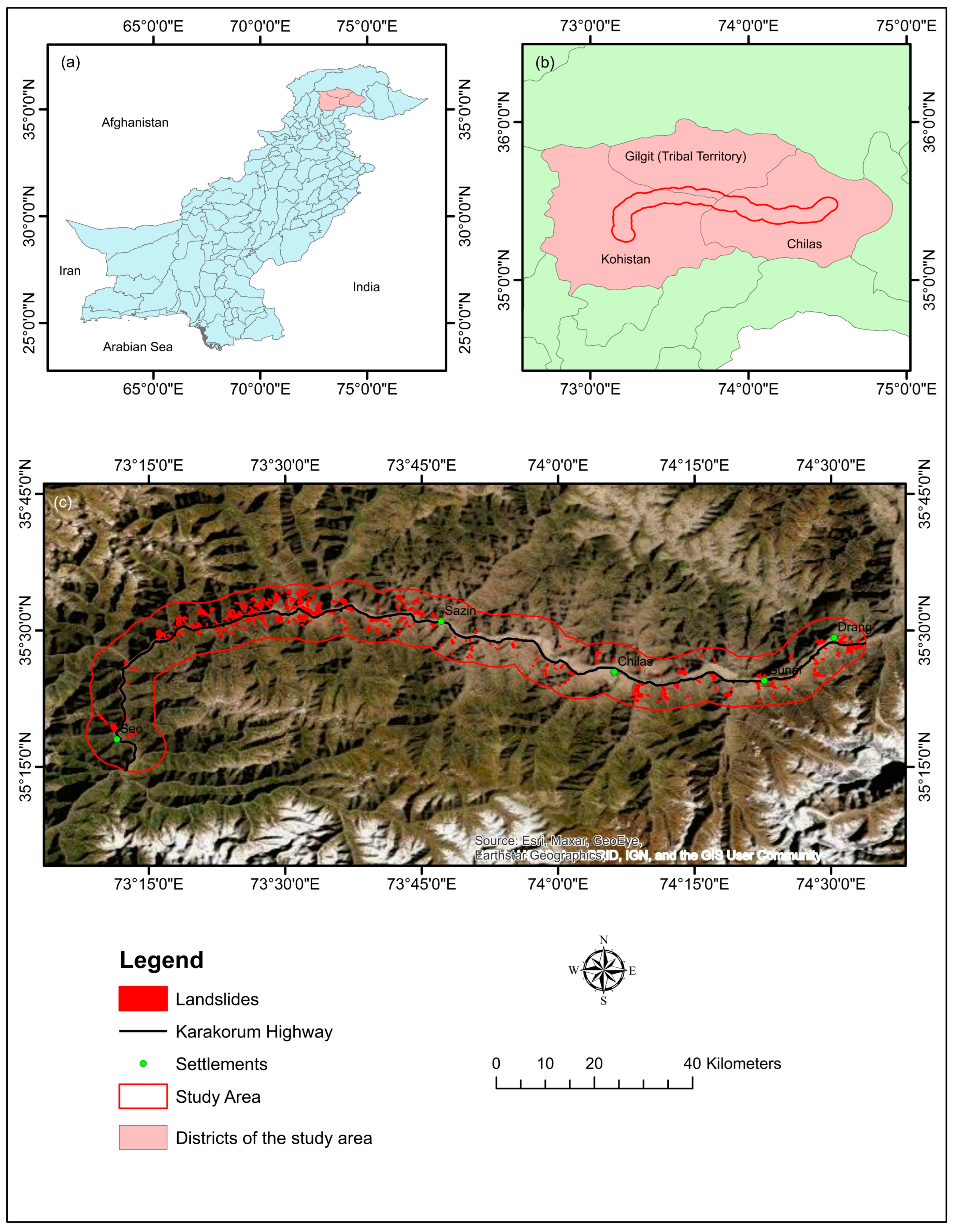
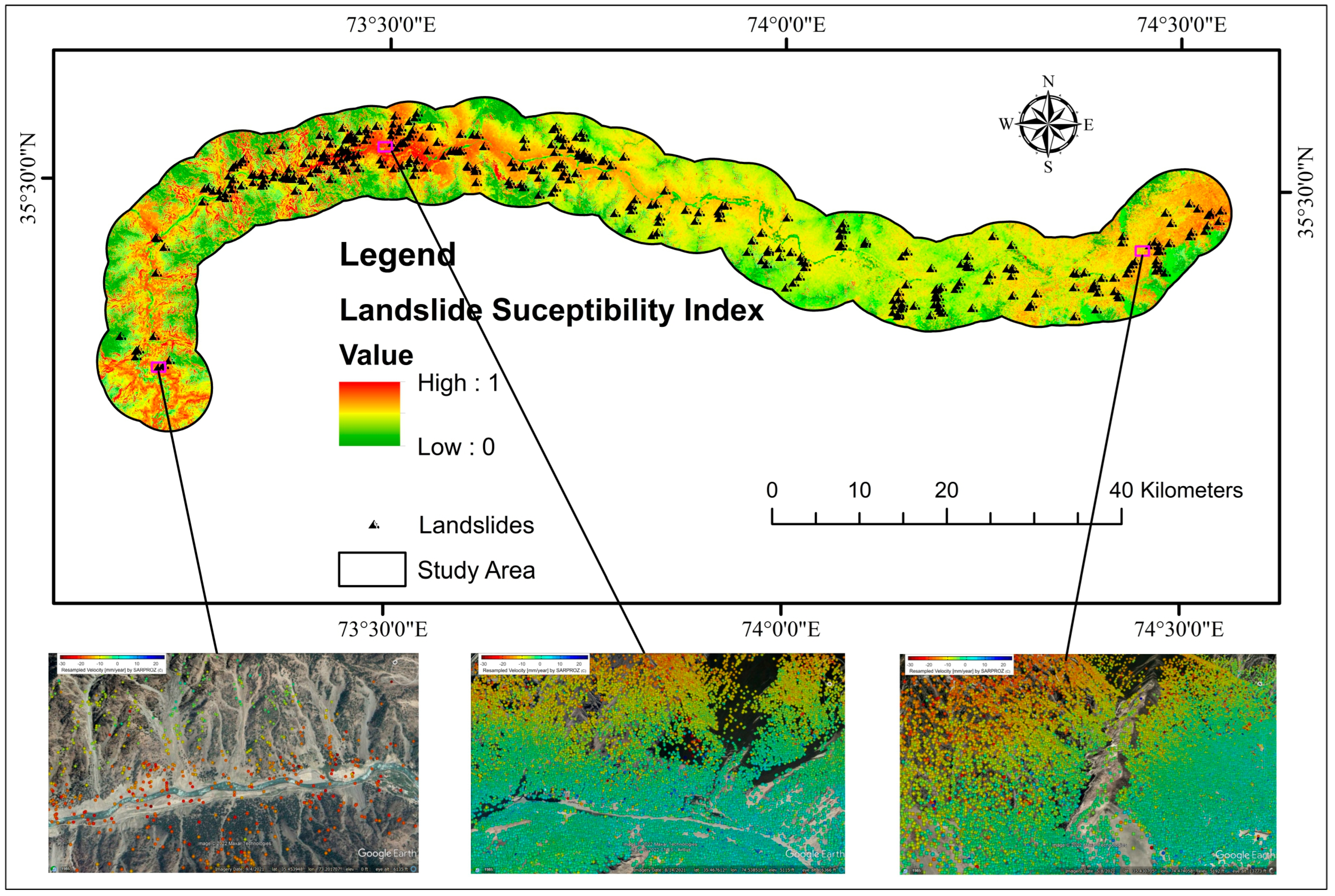
2.1. Study Area
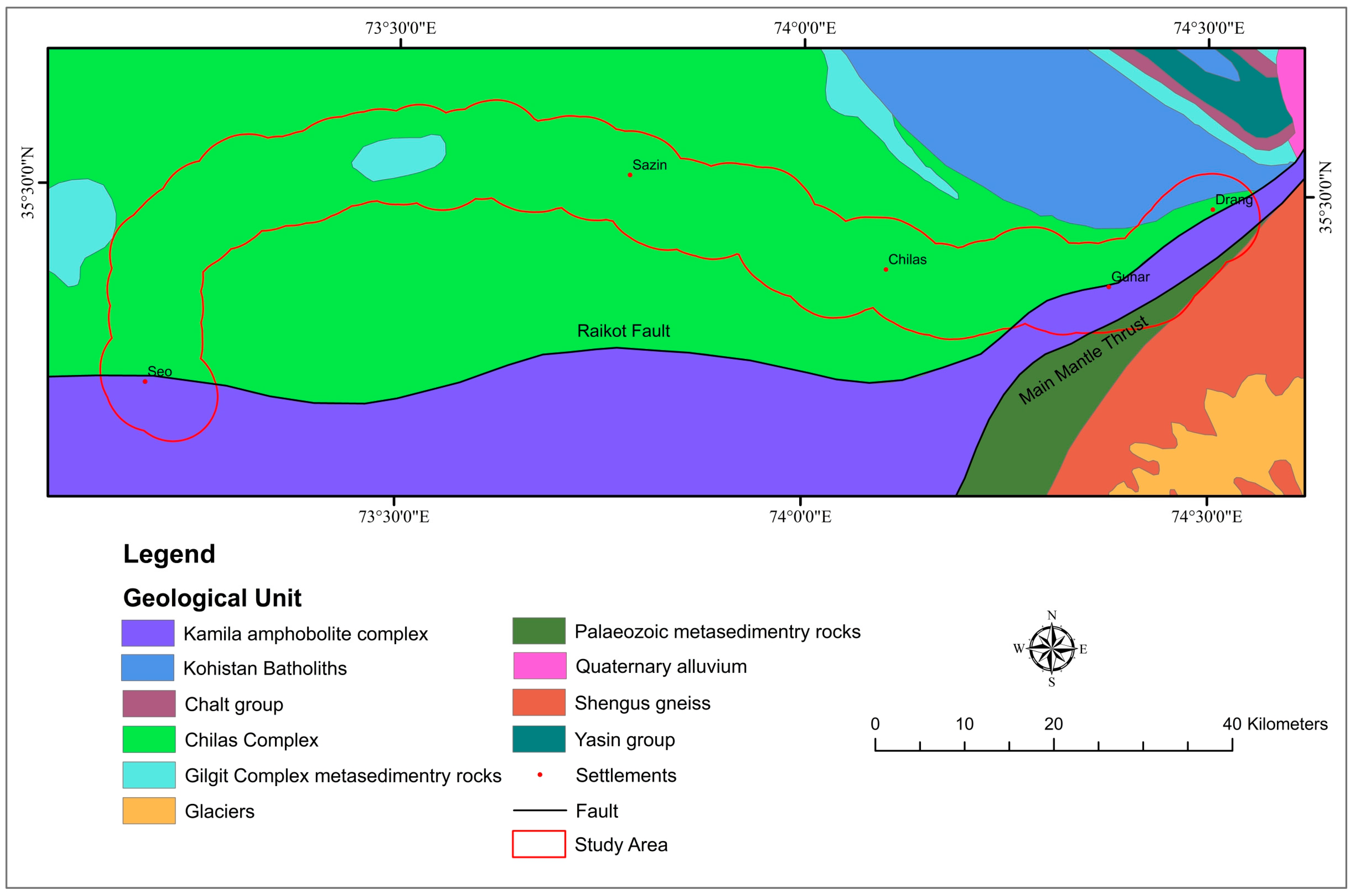
2.2. Geological Setting of the Area
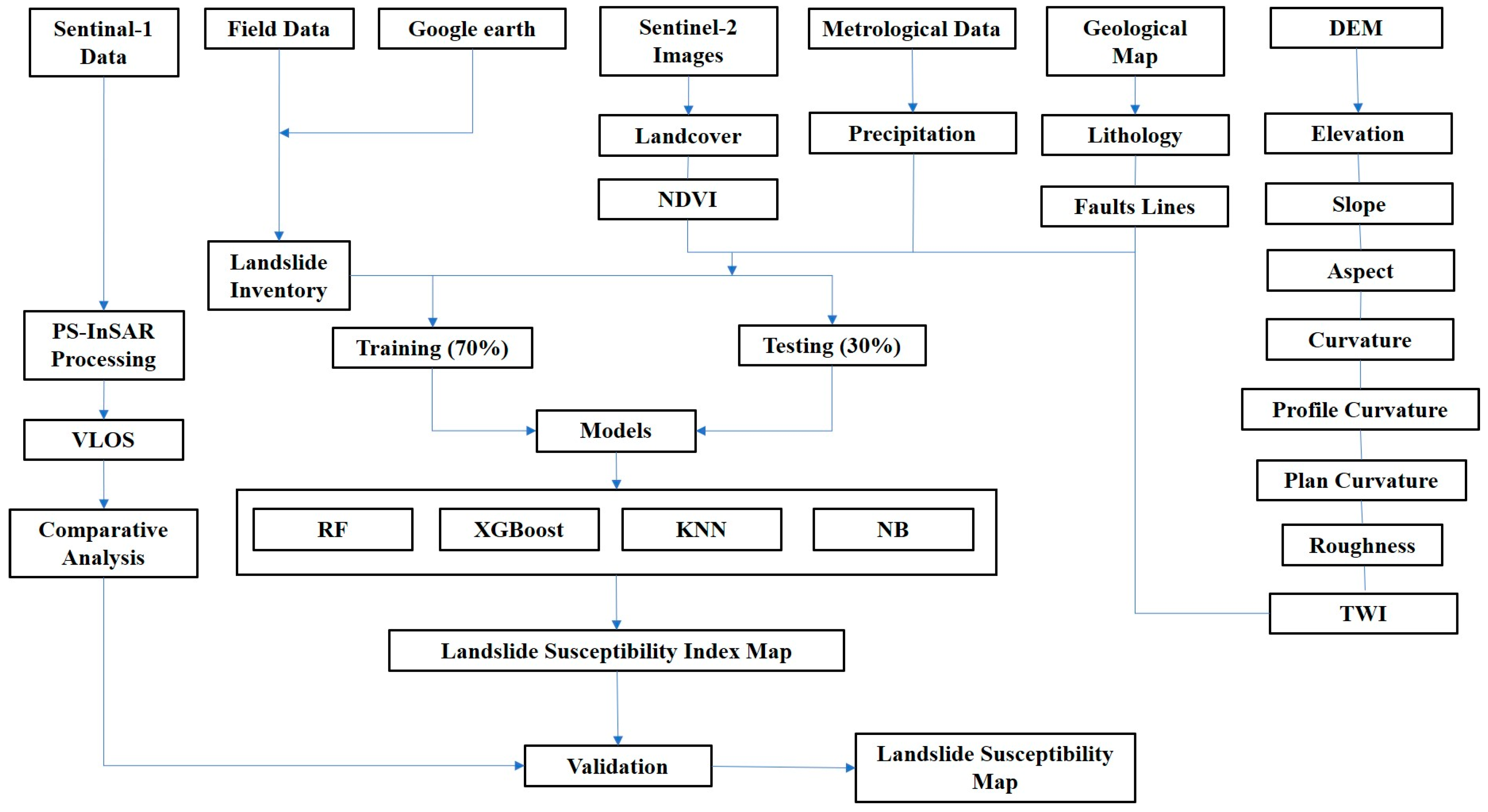
2.3. Landslide Susceptibility Mapping
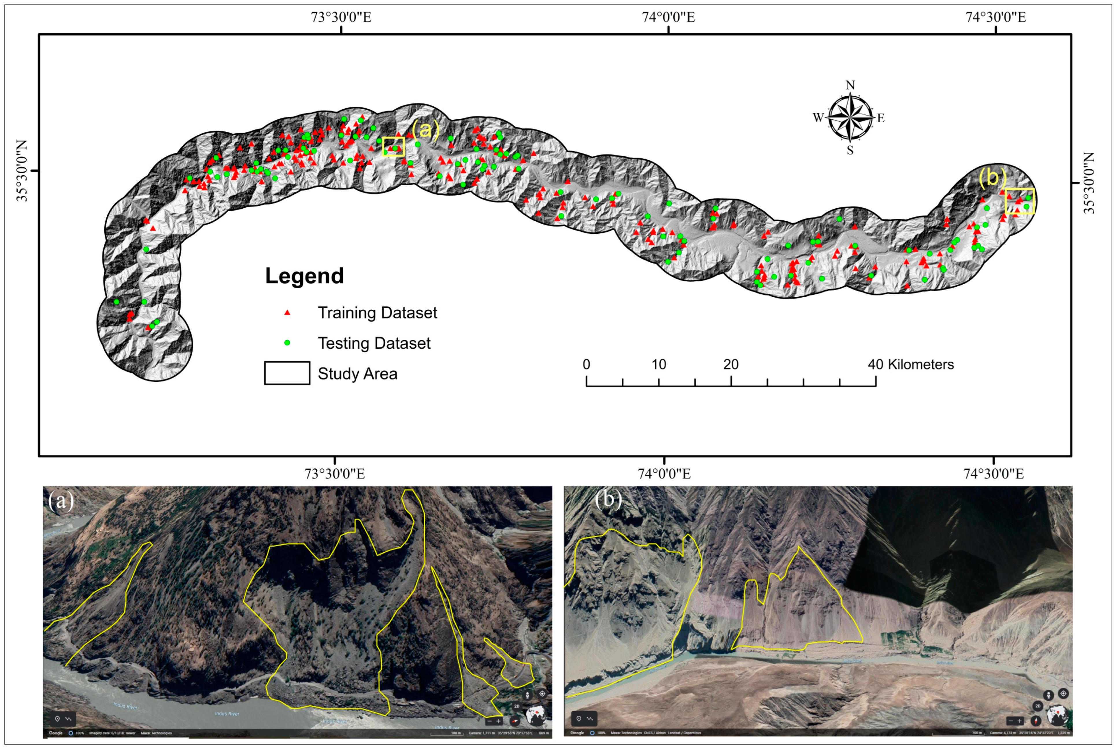
2.4. Landslide Inventory
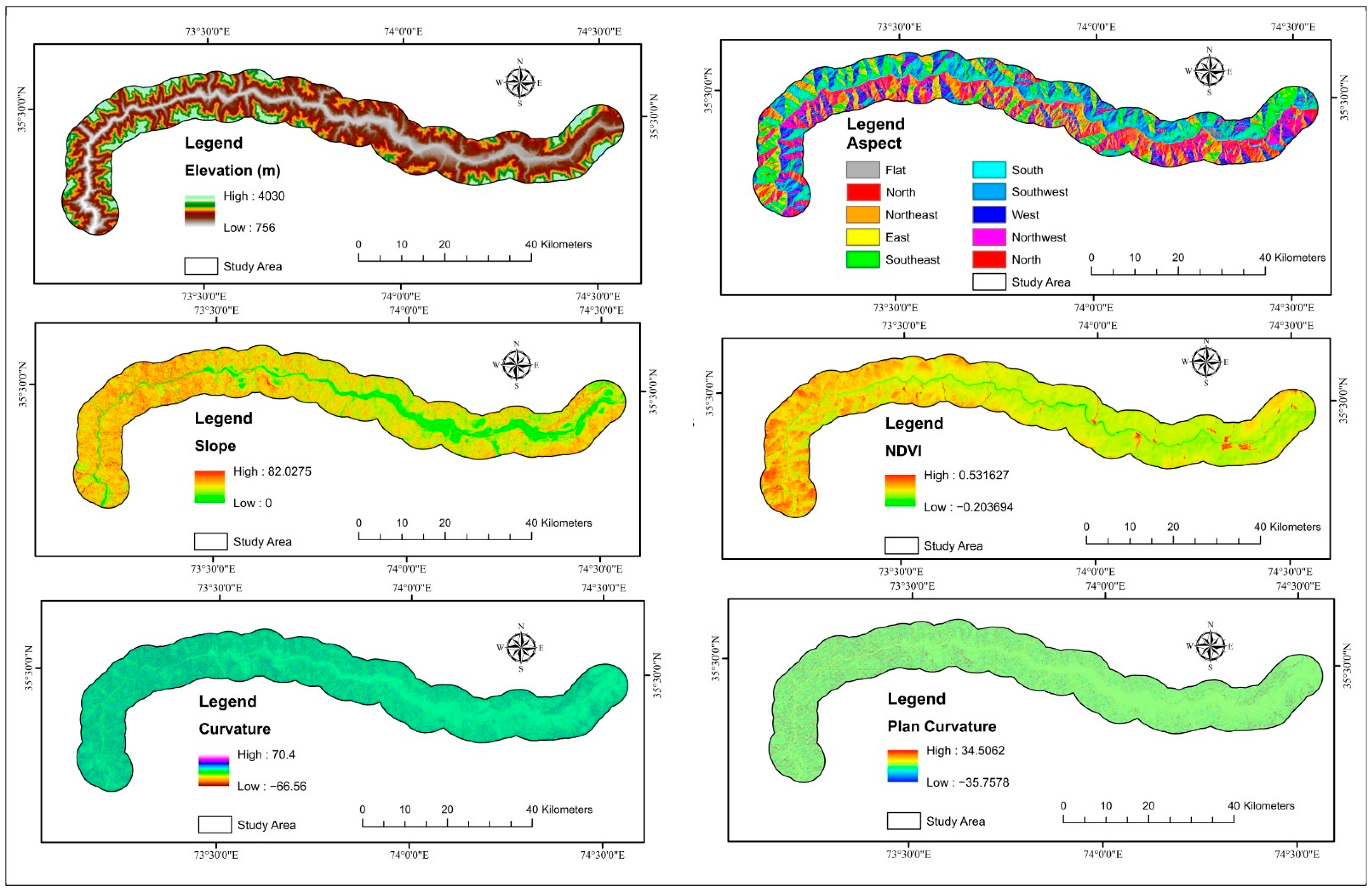
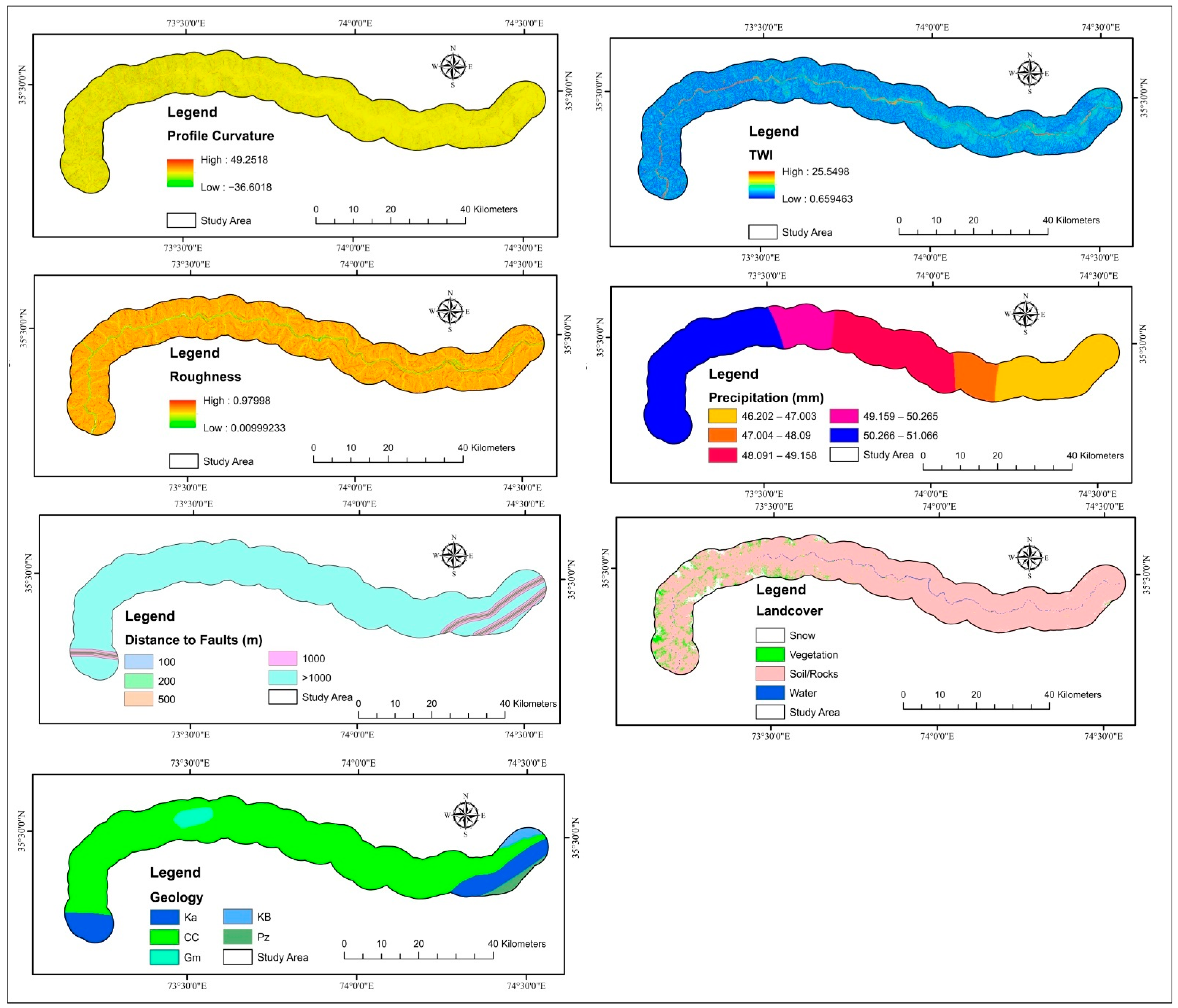
2.5. Landslide Causative Factors
- The model unit in this investigation was the grid unit (12.5 m). The spatial resolution of DEM and RS data corresponds to 12.5 m, and all assessment variables have been recalculated at this level.
- A condition property reached thirteen causative variables and a landslide decision attribute (1 indicates landslides, 0 indicates non-landslides), with each row creating an object.
- Each column represents an object’s attribute and has been converted into training (70%) and testing the two-dimensional matrix (30%). Training data were used to assemble the models, and test data was used to make forecasts.
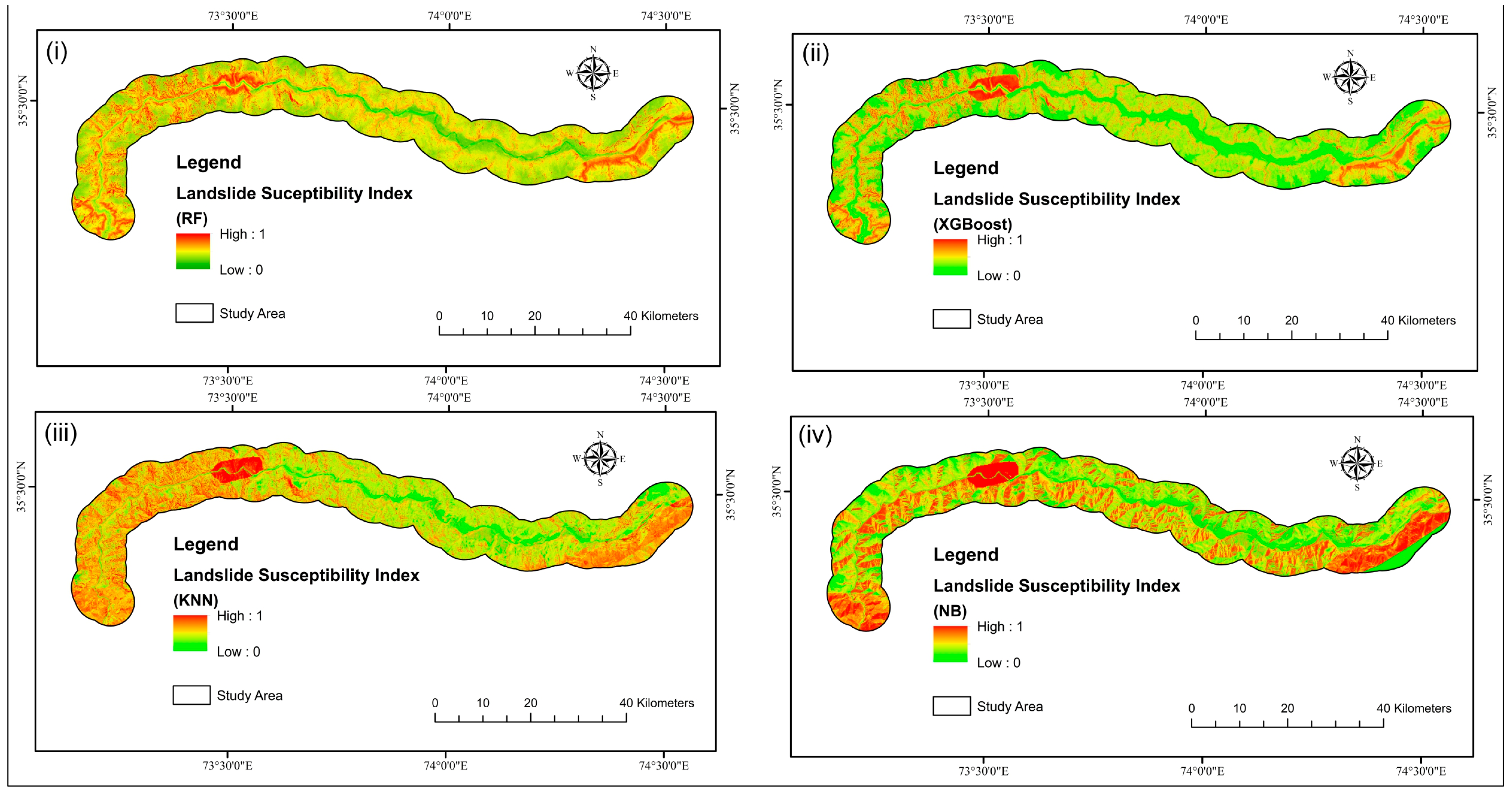
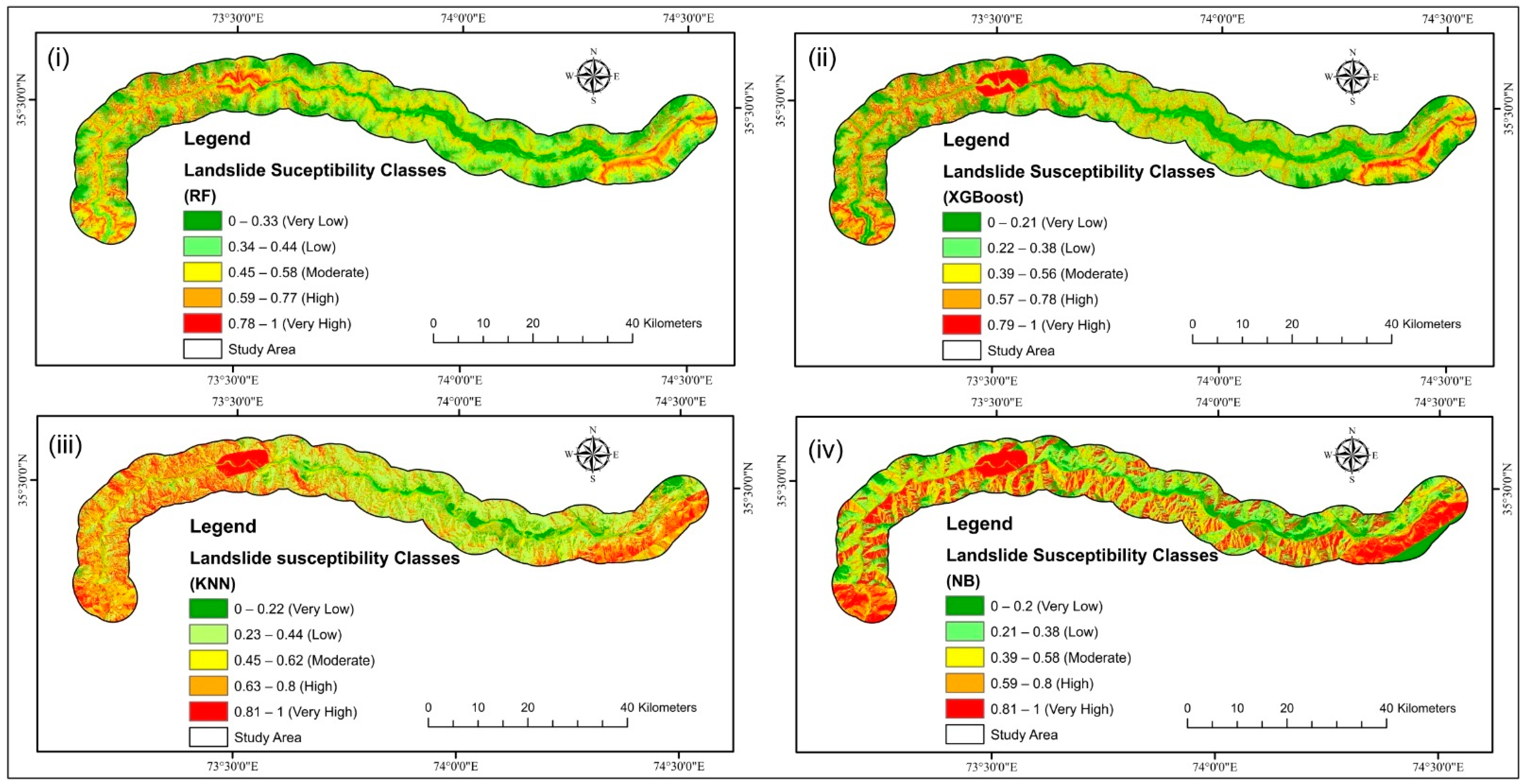
- The landslide susceptibility index maps were created using the forecast values of every model unit per group. The findings of the four algorithms were exported into GIS.
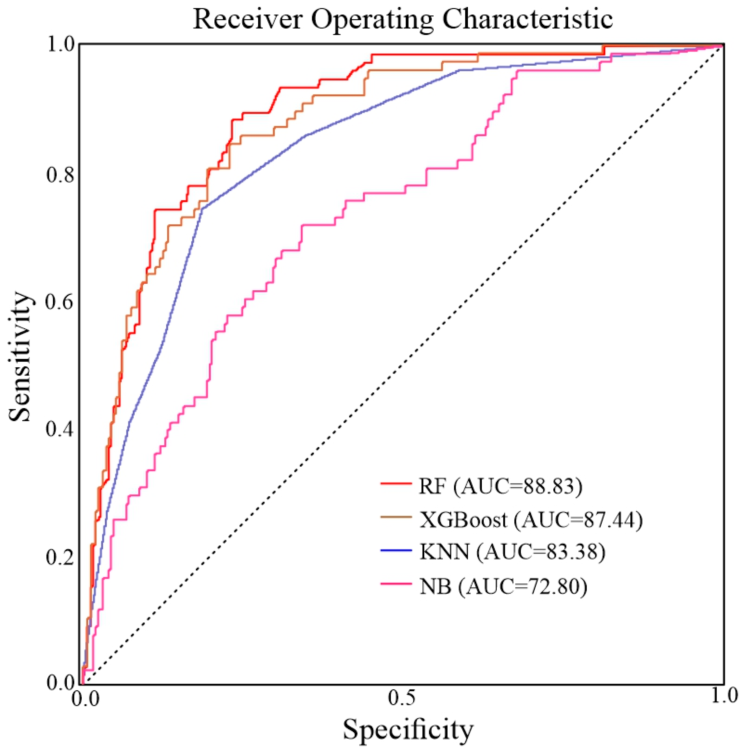
- The Jenks natural breaks [102] classifications were used to categorize LS: very low, low, moderate, high, and very high. The ROC curve and the area under the ROC curve were used to test the four models.
2.6. RF
2.7. XGBoost
- They optimize their loss function.
- The candidate split value may be quickly and accurately generated using the parallel approximation histogram method.
- In addition to a novel sparsity-aware linear tree learning algorithm, they offer an efficient cache-aware block structure for out-of-core tree learning.
2.8. KNN
2.9. NB
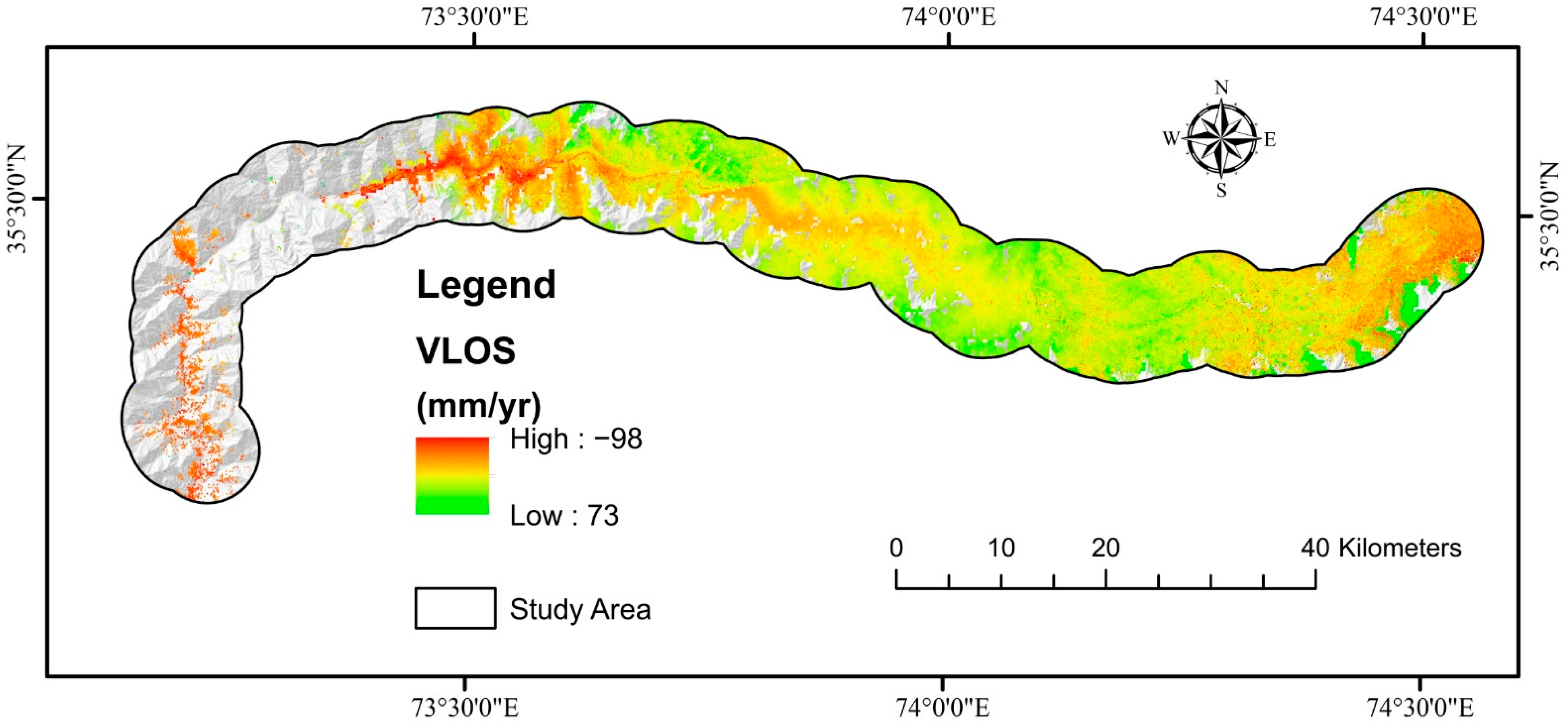
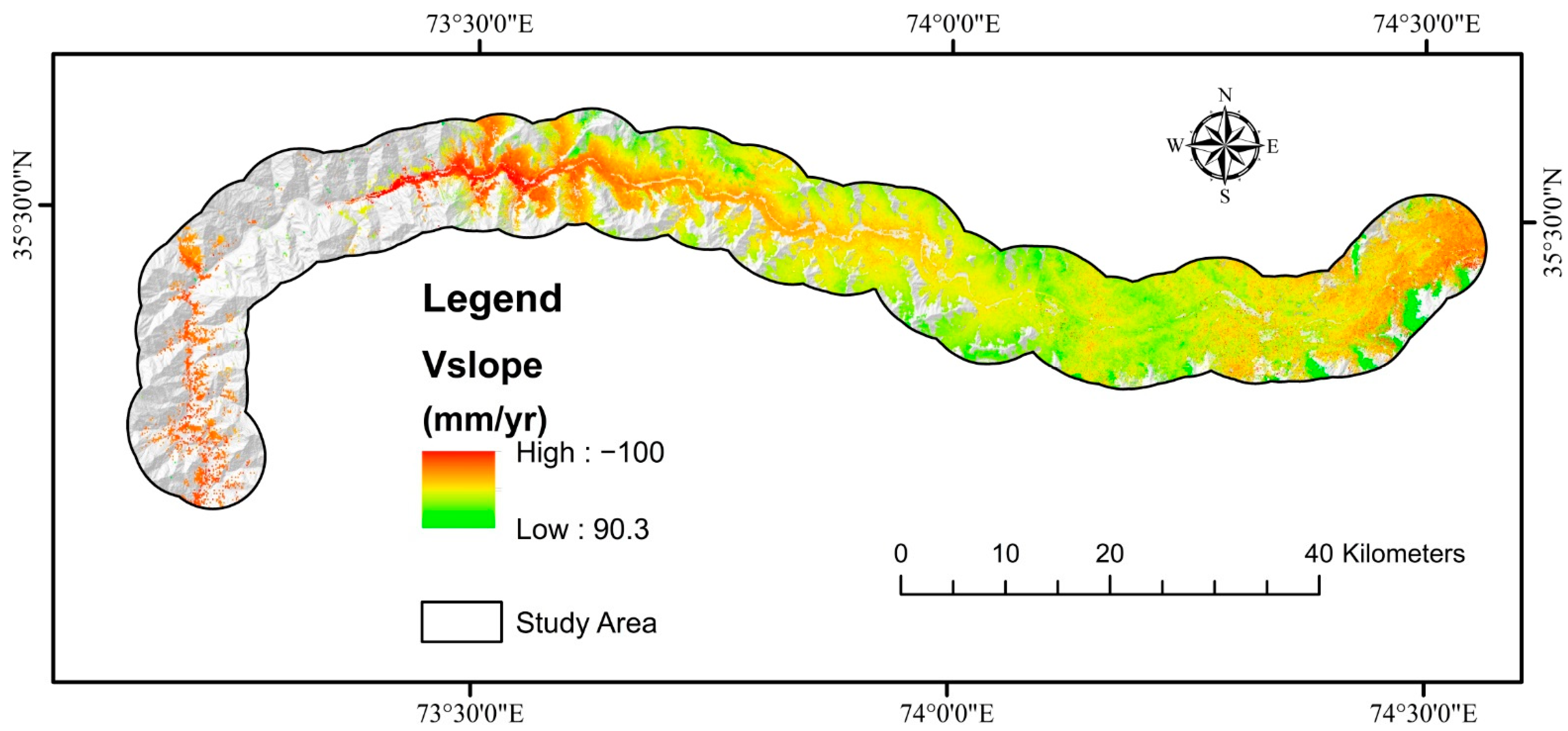
2.10. PS-InSAR
3. Results
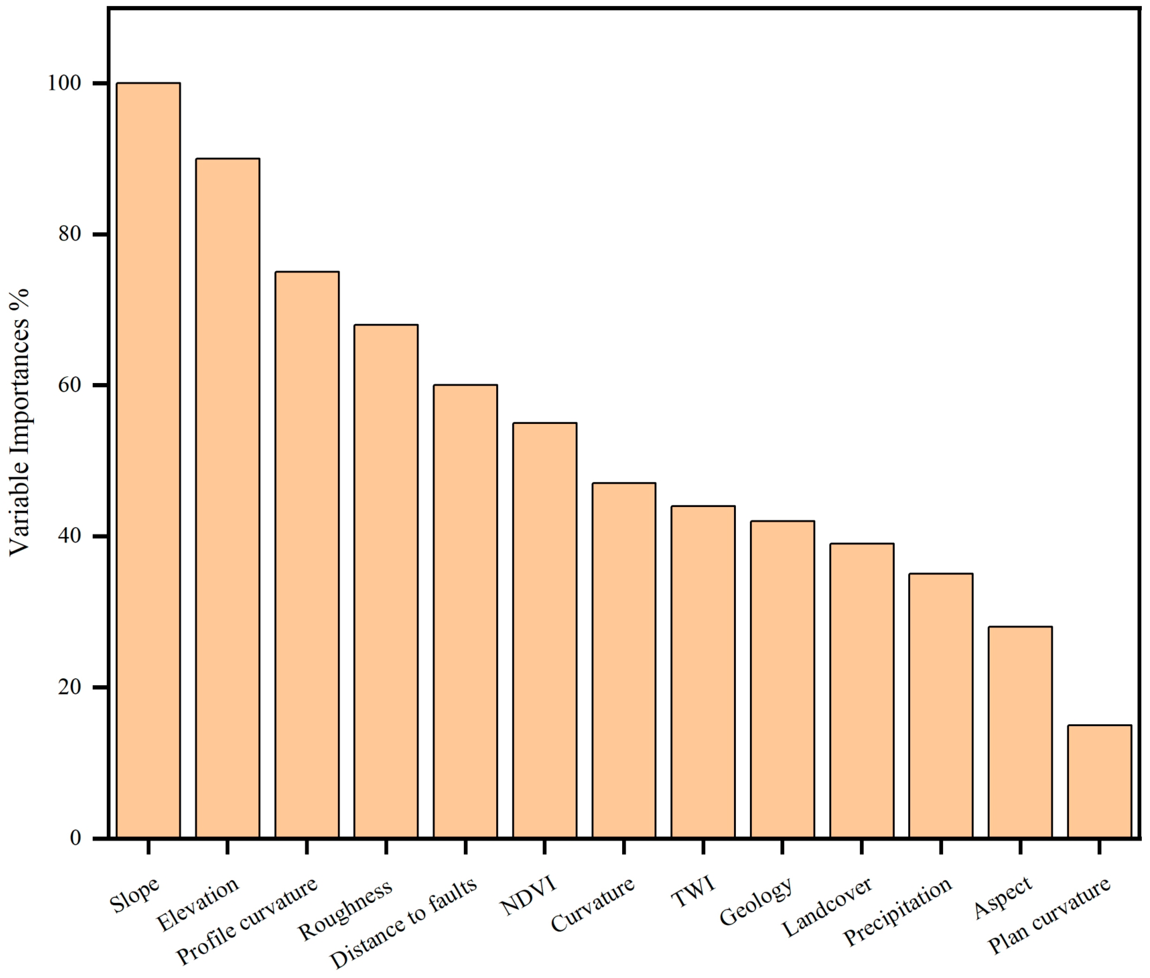
3.1. The Significance of Landslide Variables
3.2. PS-InSAR Based Validation
4. Discussion
5. Conclusions
Author Contributions
Funding
Institutional Review Board Statement
Informed Consent Statement
Data Availability Statement
Acknowledgments
Conflicts of Interest
References
- Reichenbach, P.; Rossi, M.; Malamud, B.D.; Mihir, M.; Guzzetti, F. A review of statistically-based landslide susceptibility models. Earth-Sci. Rev. 2018, 180, 60–91. [Google Scholar] [CrossRef]
- Zhou, C.; Yin, K.; Cao, Y.; Ahmed, B.; Li, Y.; Catani, F.; Pourghasemi, H.R. Landslide susceptibility modeling applying machine learning methods: A case study from Longju in the Three Gorges Reservoir area, China. Comput. Geosci. 2018, 112, 23–37. [Google Scholar] [CrossRef] [Green Version]
- Guzzetti, F.; Carrara, A.; Cardinali, M.; Reichenbach, P. Landslide hazard evaluation: A review of current techniques and their application in a multi-scale study, Central Italy. Geomorphology 1999, 31, 181–216. [Google Scholar] [CrossRef]
- Wu, Y.; Li, W.; Liu, P.; Bai, H.; Wang, Q.; He, J.; Liu, Y.; Sun, S. Application of analytic hierarchy process model for landslide susceptibility mapping in the Gangu County, Gansu Province, China. Environ. Earth Sci. 2016, 75, 422. [Google Scholar] [CrossRef]
- Wang, Q.; Li, W. A GIS-based comparative evaluation of analytical hierarchy process and frequency ratio models for landslide susceptibility mapping. Phys. Geogr. 2017, 38, 318–337. [Google Scholar] [CrossRef]
- Nguyen, T.T.N.; Liu, C.-C. A new approach using AHP to generate landslide susceptibility maps in the Chen-Yu-Lan Watershed, Taiwan. Sensors 2019, 19, 505. [Google Scholar] [CrossRef] [Green Version]
- Neuhäuser, B.; Damm, B.; Terhorst, B. GIS-based assessment of landslide susceptibility on the base of the weights-of-evidence model. Landslides 2012, 9, 511–528. [Google Scholar] [CrossRef]
- Razavizadeh, S.; Solaimani, K.; Massironi, M.; Kavian, A. Mapping landslide susceptibility with frequency ratio, statistical index, and weights of evidence models: A case study in northern Iran. Environ. Earth Sci. 2017, 76, 499. [Google Scholar] [CrossRef]
- Khan, H.; Shafique, M.; Khan, M.A.; Bacha, M.A.; Shah, S.U.; Calligaris, C. Landslide susceptibility assessment using Frequency Ratio, a case study of northern Pakistan. Egypt. J. Remote Sens. Space Sci. 2019, 22, 11–24. [Google Scholar] [CrossRef]
- Rossi, M.; Guzzetti, F.; Reichenbach, P.; Mondini, A.C.; Peruccacci, S. Optimal landslide susceptibility zonation based on multiple forecasts. Geomorphology 2010, 114, 129–142. [Google Scholar] [CrossRef]
- Hussain, M.L.; Shafique, M.; Bacha, A.S.; Chen, X.-Q.; Chen, H.-Y. Landslide inventory and susceptibility assessment using multiple statistical approaches along the Karakoram highway, northern Pakistan. J. Mt. Sci. 2021, 18, 583–598. [Google Scholar] [CrossRef]
- Iqbal, J.; Cui, P.; Hussain, M.L.; Pourghasemi, H.R.; Pradhan, B. Landslide susceptibility assessment along the dubair-dud ishal section of the karakoram highway, northwestern himalayas, pakistan. Acta Geodyn. Geomater 2021, 18, 137–155. [Google Scholar] [CrossRef]
- Rashid, B.; Iqbal, J.; Su, L.-J. Landslide susceptibility analysis of Karakoram highway using analytical hierarchy process and scoops 3D. J. Mt. Sci. 2020, 17, 1596–1612. [Google Scholar] [CrossRef]
- Ali, S.; Biermanns, P.; Haider, R.; Reicherter, K. Landslide susceptibility mapping by using a geographic information system (GIS) along the China–Pakistan Economic Corridor (Karakoram Highway), Pakistan. Nat. Hazards Earth Syst. Sci. 2019, 19, 999–1022. [Google Scholar] [CrossRef] [Green Version]
- Regmi, A.D.; Devkota, K.C.; Yoshida, K.; Pradhan, B.; Pourghasemi, H.R.; Kumamoto, T.; Akgun, A. Application of frequency ratio, statistical index, and weights-of-evidence models and their comparison in landslide susceptibility mapping in Central Nepal Himalaya. Arab. J. Geosci. 2014, 7, 725–742. [Google Scholar] [CrossRef]
- Shirzadi, A.; Chapi, K.; Shahabi, H.; Solaimani, K.; Kavian, A.; Ahmad, B.B. Rock fall susceptibility assessment along a mountainous road: An evaluation of bivariate statistic, analytical hierarchy process and frequency ratio. Environ. Earth Sci. 2017, 76, 152. [Google Scholar] [CrossRef]
- Achour, Y.; Pourghasemi, H.R. How do machine learning techniques help in increasing accuracy of landslide susceptibility maps? Geosci. Front. 2020, 11, 871–883. [Google Scholar] [CrossRef]
- Kumar, R.; Anbalagan, R. Landslide susceptibility mapping using analytical hierarchy process (AHP) in Tehri reservoir rim region, Uttarakhand. J. Geol. Soc. India 2016, 87, 271–286. [Google Scholar] [CrossRef]
- Tien Bui, D.; Pradhan, B.; Lofman, O.; Revhaug, I. Landslide susceptibility assessment in vietnam using support vector machines, decision tree, and Naive Bayes Models. Math. Probl. Eng. 2012, 2012, 974638. [Google Scholar] [CrossRef] [Green Version]
- Park, S.; Choi, C.; Kim, B.; Kim, J. Landslide susceptibility mapping using frequency ratio, analytic hierarchy process, logistic regression, and artificial neural network methods at the Inje area, Korea. Environ. Earth Sci. 2013, 68, 1443–1464. [Google Scholar] [CrossRef]
- Tengtrairat, N.; Woo, W.L.; Parathai, P.; Aryupong, C.; Jitsangiam, P.; Rinchumphu, D. Automated landslide-risk prediction using web gis and machine learning models. Sensors 2021, 21, 4620. [Google Scholar] [CrossRef] [PubMed]
- Mandal, S.; Mandal, K. Modeling and mapping landslide susceptibility zones using GIS based multivariate binary logistic regression (LR) model in the Rorachu river basin of eastern Sikkim Himalaya, India. Modeling Earth Syst. Environ. 2018, 4, 69–88. [Google Scholar] [CrossRef]
- Youssef, A.M.; Pourghasemi, H.R.; Pourtaghi, Z.S.; Al-Katheeri, M.M. Landslide susceptibility mapping using random forest, boosted regression tree, classification and regression tree, and general linear models and comparison of their performance at Wadi Tayyah Basin, Asir Region, Saudi Arabia. Landslides 2016, 13, 839–856. [Google Scholar] [CrossRef]
- Pourghasemi, H.R.; Rahmati, O. Prediction of the landslide susceptibility: Which algorithm, which precision? Catena 2018, 162, 177–192. [Google Scholar] [CrossRef]
- Park, S.; Kim, J. Landslide susceptibility mapping based on random forest and boosted regression tree models, and a comparison of their performance. Appl. Sci. 2019, 9, 942. [Google Scholar] [CrossRef] [Green Version]
- Taalab, K.; Cheng, T.; Zhang, Y. Mapping landslide susceptibility and types using Random Forest. Big Earth Data 2018, 2, 159–178. [Google Scholar] [CrossRef]
- Hussain, M.A.; Chen, Z.; Wang, R.; Shoaib, M. PS-InSAR-Based Validated Landslide Susceptibility Mapping along Karakorum Highway, Pakistan. Remote Sens. 2021, 13, 4129. [Google Scholar] [CrossRef]
- Hussain, M.A.; Chen, Z.; Wang, R.; Shah, S.U.; Shoaib, M.; Ali, N.; Xu, D.; Ma, C. Landslide Susceptibility Mapping using Machine Learning Algorithm. Civ. Eng. J. 2022, 8, 209–224. [Google Scholar] [CrossRef]
- Sevgen, E.; Kocaman, S.; Nefeslioglu, H.A.; Gokceoglu, C.J.S. A novel performance assessment approach using photogrammetric techniques for landslide susceptibility mapping with logistic regression, ANN and random forest. Sensors 2019, 19, 3940. [Google Scholar] [CrossRef] [Green Version]
- Felicísimo, Á.M.; Cuartero, A.; Remondo, J.; Quirós, E. Mapping landslide susceptibility with logistic regression, multiple adaptive regression splines, classification and regression trees, and maximum entropy methods: A comparative study. Landslides 2013, 10, 175–189. [Google Scholar] [CrossRef]
- Conoscenti, C.; Ciaccio, M.; Caraballo-Arias, N.A.; Gómez-Gutiérrez, Á.; Rotigliano, E.; Agnesi, V. Assessment of susceptibility to earth-flow landslide using logistic regression and multivariate adaptive regression splines: A case of the Belice River basin (western Sicily, Italy). Geomorphology 2015, 242, 49–64. [Google Scholar] [CrossRef]
- Vorpahl, P.; Elsenbeer, H.; Märker, M.; Schröder, B. How can statistical models help to determine driving factors of landslides? Ecol. Model. 2012, 239, 27–39. [Google Scholar] [CrossRef]
- Kalantar, B.; Pradhan, B.; Naghibi, S.A.; Motevalli, A.; Mansor, S. Assessment of the effects of training data selection on the landslide susceptibility mapping: A comparison between support vector machine (SVM), logistic regression (LR) and artificial neural networks (ANN). Geomat. Nat. Hazards Risk 2018, 9, 49–69. [Google Scholar] [CrossRef]
- Ma, J.; Wang, Y.; Niu, X.; Jiang, S.; Liu, Z. A comparative study of mutual information-based input variable selection strategies for the displacement prediction of seepage-driven landslides using optimized support vector regression. Stoch. Environ. Res. Risk Assess. 2022, 1, 1–21. [Google Scholar] [CrossRef]
- Ghasemian, B.; Shahabi, H.; Shirzadi, A.; Al-Ansari, N.; Jaafari, A.; Kress, V.R.; Geertsema, M.; Renoud, S.; Ahmad, A. A robust deep-learning model for landslide susceptibility mapping: A case study of Kurdistan Province, Iran. Sensors 2022, 22, 1573. [Google Scholar] [CrossRef]
- Pham, B.T.; Pradhan, B.; Bui, D.T.; Prakash, I.; Dholakia, M. A comparative study of different machine learning methods for landslide susceptibility assessment: A case study of Uttarakhand area (India). Environ. Model. Softw. 2016, 84, 240–250. [Google Scholar] [CrossRef]
- Pham, B.T.; Tien Bui, D.; Pourghasemi, H.R.; Indra, P.; Dholakia, M. Landslide susceptibility assesssment in the Uttarakhand area (India) using GIS: A comparison study of prediction capability of naïve bayes, multilayer perceptron neural networks, and functional trees methods. Theor. Appl. Climatol. 2017, 128, 255–273. [Google Scholar] [CrossRef]
- Aghdam, I.N.; Varzandeh, M.H.M.; Pradhan, B. Landslide susceptibility mapping using an ensemble statistical index (Wi) and adaptive neuro-fuzzy inference system (ANFIS) model at Alborz Mountains (Iran). Environ. Earth Sci. 2016, 75, 553. [Google Scholar] [CrossRef]
- Dehnavi, A.; Aghdam, I.N.; Pradhan, B.; Varzandeh, M.H.M. A new hybrid model using step-wise weight assessment ratio analysis (SWARA) technique and adaptive neuro-fuzzy inference system (ANFIS) for regional landslide hazard assessment in Iran. Catena 2015, 135, 122–148. [Google Scholar] [CrossRef]
- Mehrabi, M.; Pradhan, B.; Moayedi, H.; Alamri, A. Optimizing an adaptive neuro-fuzzy inference system for spatial prediction of landslide susceptibility using four state-of-the-art metaheuristic techniques. Sensors 2020, 20, 1723. [Google Scholar] [CrossRef] [Green Version]
- Kumar, R.; Anbalagan, R. Landslide susceptibility zonation in part of Tehri reservoir region using frequency ratio, fuzzy logic and GIS. J. Earth Syst. Sci. 2015, 124, 431–448. [Google Scholar] [CrossRef]
- Aditian, A.; Kubota, T.; Shinohara, Y. Comparison of GIS-based landslide susceptibility models using frequency ratio, logistic regression, and artificial neural network in a tertiary region of Ambon, Indonesia. Geomorphology 2018, 318, 101–111. [Google Scholar] [CrossRef]
- Arnone, E.; Francipane, A.; Scarbaci, A.; Puglisi, C.; Noto, L.V. Effect of raster resolution and polygon-conversion algorithm on landslide susceptibility mapping. Environ. Model. Softw. 2016, 84, 467–481. [Google Scholar] [CrossRef]
- Bui, D.T.; Moayedi, H.; Kalantar, B.; Osouli, A.; Pradhan, B.; Nguyen, H.; Rashid, A.S.A. A novel swarm intelligence—Harris hawks optimization for spatial assessment of landslide susceptibility. Sensors 2019, 19, 3590. [Google Scholar] [CrossRef] [PubMed] [Green Version]
- Moayedi, H.; Osouli, A.; Tien Bui, D.; Foong, L.K. Spatial landslide susceptibility assessment based on novel neural-metaheuristic geographic information system based ensembles. Sensors 2019, 19, 4698. [Google Scholar] [CrossRef] [Green Version]
- Roshani, M.; Sattari, M.A.; Ali, P.J.M.; Roshani, G.H.; Nazemi, B.; Corniani, E.; Nazemi, E. Application of GMDH neural network technique to improve measuring precision of a simplified photon attenuation based two-phase flowmeter. Flow Meas. Instrum. 2020, 75, 101804. [Google Scholar] [CrossRef]
- Charandabi, S.E.; Kamyar, K. Prediction of Cryptocurrency Price Index Using Artificial Neural Networks: A Survey of the Literature. Eur. J. Bus. Manag. Res. 2021, 6, 17–20. [Google Scholar] [CrossRef]
- Park, N.-W. Using maximum entropy modeling for landslide susceptibility mapping with multiple geoenvironmental data sets. Environ. Earth Sci. 2015, 73, 937–949. [Google Scholar] [CrossRef]
- Kornejady, A.; Ownegh, M.; Bahremand, A. Landslide susceptibility assessment using maximum entropy model with two different data sampling methods. Catena 2017, 152, 144–162. [Google Scholar] [CrossRef]
- Wu, X.; Ren, F.; Niu, R. Landslide susceptibility assessment using object mapping units, decision tree, and support vector machine models in the Three Gorges of China. Environ. Earth Sci. 2014, 71, 4725–4738. [Google Scholar] [CrossRef]
- Shirzadi, A.; Soliamani, K.; Habibnejhad, M.; Kavian, A.; Chapi, K.; Shahabi, H.; Chen, W.; Khosravi, K.; Thai Pham, B.; Pradhan, B. Novel GIS based machine learning algorithms for shallow landslide susceptibility mapping. Sensors 2018, 18, 3777. [Google Scholar] [CrossRef] [PubMed]
- Qing, F.; Zhao, Y.; Meng, X.; Su, X.; Qi, T.; Yue, D. Application of Machine Learning to Debris Flow Susceptibility Mapping along the China–Pakistan Karakoram Highway. Remote Sens. 2020, 12, 2933. [Google Scholar] [CrossRef]
- Pradhan, A.M.S.; Kim, Y.-T. Rainfall-induced shallow landslide susceptibility mapping at two adjacent catchments using advanced machine learning algorithms. ISPRS Int. J. Geo-Inf. 2020, 9, 569. [Google Scholar] [CrossRef]
- Merghadi, A.; Yunus, A.P.; Dou, J.; Whiteley, J.; ThaiPham, B.; Bui, D.T.; Avtar, R.; Abderrahmane, B. Machine learning methods for landslide susceptibility studies: A comparative overview of algorithm performance. Earth-Sci. Rev. 2020, 207, 103225. [Google Scholar] [CrossRef]
- Sahin, E.K. Comparative analysis of gradient boosting algorithms for landslide susceptibility mapping. Geocarto Int. 2020, 35, 1–25. [Google Scholar] [CrossRef]
- Yan, F.; Zhang, Q.; Ye, S.; Ren, B. A novel hybrid approach for landslide susceptibility mapping integrating analytical hierarchy process and normalized frequency ratio methods with the cloud model. Geomorphology 2019, 327, 170–187. [Google Scholar] [CrossRef]
- Pourghasemi, H.R.; Gayen, A.; Panahi, M.; Rezaie, F.; Blaschke, T. Multi-hazard probability assessment and mapping in Iran. Sci. Total Environ. 2019, 692, 556–571. [Google Scholar] [CrossRef]
- Nohani, E.; Moharrami, M.; Sharafi, S.; Khosravi, K.; Pradhan, B.; Pham, B.T.; Lee, S.; Melesse, A.M. Landslide susceptibility mapping using different GIS-based bivariate models. Water 2019, 11, 1402. [Google Scholar] [CrossRef] [Green Version]
- Scaioni, M.; Longoni, L.; Melillo, V.; Papini, M. Remote sensing for landslide investigations: An overview of recent achievements and perspectives. Remote Sens. 2014, 6, 9600–9652. [Google Scholar] [CrossRef] [Green Version]
- Corsini, A.; Borgatti, L.; Cervi, F.; Dahne, A.; Ronchetti, F.; Sterzai, P. Estimating mass-wasting processes in active earth slides–earth flows with time-series of High-Resolution DEMs from photogrammetry and airborne LiDAR. Nat. Hazards Earth Syst. Sci. 2009, 9, 433–439. [Google Scholar] [CrossRef]
- Lai, J.-S.; Tsai, F. Improving GIS-based landslide susceptibility assessments with multi-temporal remote sensing and machine learning. Sensors 2019, 19, 3717. [Google Scholar] [CrossRef] [PubMed] [Green Version]
- Schlögel, R.; Doubre, C.; Malet, J.-P.; Masson, F. Landslide deformation monitoring with ALOS/PALSAR imagery: A D-InSAR geomorphological interpretation method. Geomorphology 2015, 231, 314–330. [Google Scholar] [CrossRef]
- Intrieri, E.; Gigli, G.; Mugnai, F.; Fanti, R.; Casagli, N. Design and implementation of a landslide early warning system. Eng. Geol. 2012, 147, 124–136. [Google Scholar] [CrossRef] [Green Version]
- Lotfi, F.; Semiari, O. Performance Analysis and Optimization of Uplink Cellular Networks with Flexible Frame Structure. In Proceedings of the 2021 IEEE 93rd Vehicular Technology Conference (VTC2021-Spring), Helsinki, Finland, 25–28 April 2021; pp. 1–5. [Google Scholar]
- Lotfi, F.; Semiari, O.; Saad, W. Semantic-Aware Collaborative Deep Reinforcement Learning Over Wireless Cellular Networks. arXiv 2011, arXiv:2111.12064. [Google Scholar]
- Ferretti, A.; Prati, C.; Rocca, F. Nonlinear subsidence rate estimation using permanent scatterers in differential SAR interferometry. IEEE Trans. Geosci. Remote Sens. 2000, 38, 2202–2212. [Google Scholar] [CrossRef] [Green Version]
- Colesanti, C.; Ferretti, A.; Prati, C.; Rocca, F. Monitoring landslides and tectonic motions with the Permanent Scatterers Technique. Eng. Geol. 2003, 68, 3–14. [Google Scholar] [CrossRef]
- Mora, O.; Mallorqui, J.J.; Broquetas, A. Linear and nonlinear terrain deformation maps from a reduced set of interferometric SAR images. IEEE Trans. Geosci. Remote Sens. 2003, 41, 2243–2253. [Google Scholar] [CrossRef]
- Ferretti, A.; Fumagalli, A.; Novali, F.; Prati, C.; Rocca, F.; Rucci, A. A new algorithm for processing interferometric data-stacks: SqueeSAR. IEEE Trans. Geosci. Remote Sens. 2011, 49, 3460–3470. [Google Scholar] [CrossRef]
- Berardino, P.; Fornaro, G.; Lanari, R.; Sansosti, E. A new algorithm for surface deformation monitoring based on small baseline differential SAR interferograms. IEEE Trans. Geosci. Remote Sens. 2002, 40, 2375–2383. [Google Scholar] [CrossRef] [Green Version]
- Zhao, F.; Meng, X.; Zhang, Y.; Chen, G.; Su, X.; Yue, D. Landslide susceptibility mapping of karakorum highway combined with the application of SBAS-InSAR technology. Sensors 2019, 19, 2685. [Google Scholar] [CrossRef] [Green Version]
- Hooper, A.; Segall, P.; Zebker, H. Persistent scatterer interferometric synthetic aperture radar for crustal deformation analysis, with application to Volcán Alcedo, Galápagos. J. Geophys. Res. Solid Earth 2007, 112. [Google Scholar] [CrossRef] [Green Version]
- Crosetto, M.; Biescas, E.; Duro, J.; Closa, J.; Arnaud, A. Generation of advanced ERS and Envisat interferometric SAR products using the stable point network technique. Photogramm. Eng. Remote Sens. 2008, 74, 443–450. [Google Scholar] [CrossRef]
- Herrera, G.; Notti, D.; García-Davalillo, J.C.; Mora, O.; Cooksley, G.; Sánchez, M.; Arnaud, A.; Crosetto, M. Analysis with C-and X-band satellite SAR data of the Portalet landslide area. Landslides 2011, 8, 195–206. [Google Scholar] [CrossRef]
- Strozzi, T.; Wegmuller, U.; Keusen, H.R.; Graf, K.; Wiesmann, A. Analysis of the terrain displacement along a funicular by SAR interferometry. IEEE Geosci. Remote Sens. Lett. 2006, 3, 15–18. [Google Scholar] [CrossRef]
- Lu, P.; Stumpf, A.; Kerle, N.; Casagli, N. Object-oriented change detection for landslide rapid mapping. IEEE Geosci. Remote Sens. Lett. 2011, 8, 701–705. [Google Scholar] [CrossRef]
- Agostini, A.; Tofani, V.; Nolesini, T.; Gigli, G.; Tanteri, L.; Rosi, A.; Cardellini, S.; Casagli, N. A new appraisal of the Ancona landslide based on geotechnical investigations and stability modelling. Q. J. Eng. Geol. Hydrogeol. 2014, 47, 29–43. [Google Scholar] [CrossRef]
- Jones, D.; Brunsden, D.; Goudie, A. A preliminary geomorphological assessment of part of the Karakoram Highway. Q. J. Eng. Geol. 1983, 16, 331–355. [Google Scholar] [CrossRef]
- Bishop, M.P.; Shroder Jr, J.F.; Hickman, B.L.; Copland, L. Scale-dependent analysis of satellite imagery for characterization of glacier surfaces in the Karakoram Himalaya. Geomorphology 1998, 21, 217–232. [Google Scholar] [CrossRef]
- Derbyshire, E.; Fort, M.; Owen, L.A. Geomorphological hazards along the Karakoram highway: Khunjerab pass to the Gilgit River, northernmost Pakistan (Geomorphologische hazards entlang des Karakorum highway: Khunjerab Paß bis zum Gilgit River, nördlichstes Pakistan). Erdkunde 2001, 1, 49–71. [Google Scholar] [CrossRef]
- Korup, O.; Clague, J.J.; Hermanns, R.L.; Hewitt, K.; Strom, A.L.; Weidinger, J.T. Giant landslides, topography, and erosion. Earth Planet. Sci. Lett. 2007, 261, 578–589. [Google Scholar] [CrossRef]
- Rahman, M.; Ahmed, B.; Di, L. Landslide initiation and runout susceptibility modeling in the context of hill cutting and rapid urbanization: A combined approach of weights of evidence and spatial multi-criteria. J. Mt. Sci. 2017, 14, 1919–1937. [Google Scholar] [CrossRef]
- Bacha, A.S.; Shafique, M.; van der Werff, H. Landslide inventory and susceptibility modelling using geospatial tools, in Hunza-Nagar valley, northern Pakistan. J. Mt. Sci. 2018, 15, 1354–1370. [Google Scholar] [CrossRef]
- Ahmed, M.F.; Rogers, J.D.; Ismail, E.H. A regional level preliminary landslide susceptibility study of the upper Indus river basin. Eur. J. Remote Sens. 2014, 47, 343–373. [Google Scholar] [CrossRef] [Green Version]
- Basharat, M.; Shah, H.R.; Hameed, N. Landslide susceptibility mapping using GIS and weighted overlay method: A case study from NW Himalayas, Pakistan. Arab. J. Geosci. 2016, 9, 292. [Google Scholar] [CrossRef]
- Owen, L. Wet-sediment deformation of Quaternary and recent sediments in the Skardu Basin, Karakoram Mountains, Pakistan. In Proceedings of the Glaciotectonics: Forms and Processes; Various Meetings of the Glaciotectonics Work Group. Routledge: Norflok, UK, 1988; pp. 123–147. [Google Scholar]
- Hewitt, K. Quaternary moraines vs catastrophic rock avalanches in the Karakoram Himalaya, northern Pakistan. Quat. Res. 1999, 51, 220–237. [Google Scholar] [CrossRef]
- Searle, M.; Khan, M.A.; Fraser, J.; Gough, S.; Jan, M.Q. The tectonic evolution of the Kohistan-Karakoram collision belt along the Karakoram Highway transect, north Pakistan. Tectonics 1999, 18, 929–949. [Google Scholar] [CrossRef] [Green Version]
- Guzzetti, F.; Mondini, A.C.; Cardinali, M.; Fiorucci, F.; Santangelo, M.; Chang, K.-T. Landslide inventory maps: New tools for an old problem. Earth-Sci. Rev. 2012, 112, 42–66. [Google Scholar] [CrossRef] [Green Version]
- Paliaga, G.; Luino, F.; Turconi, L.; Faccini, F. Inventory of geo-hydrological phenomena in Genova municipality (NW Italy). J. Maps 2019, 15, 28–37. [Google Scholar] [CrossRef]
- Shafique, M.; van der Meijde, M.; Khan, M.A. A review of the 2005 Kashmir earthquake-induced landslides; from a remote sensing prospective. J. Asian Earth Sci. 2016, 118, 68–80. [Google Scholar] [CrossRef]
- Ilia, I.; Tsangaratos, P. Applying weight of evidence method and sensitivity analysis to produce a landslide susceptibility map. Landslides 2016, 13, 379–397. [Google Scholar] [CrossRef]
- Chen, W.; Pourghasemi, H.R.; Panahi, M.; Kornejady, A.; Wang, J.; Xie, X.; Cao, S. Spatial prediction of landslide susceptibility using an adaptive neuro-fuzzy inference system combined with frequency ratio, generalized additive model, and support vector machine techniques. Geomorphology 2017, 297, 69–85. [Google Scholar] [CrossRef]
- Riaz, M.T.; Basharat, M.; Hameed, N.; Shafique, M.; Luo, J. A data-driven approach to landslide-susceptibility mapping in mountainous terrain: Case study from the Northwest Himalayas, Pakistan. Nat. Hazards Rev. 2018, 19, 05018007. [Google Scholar] [CrossRef]
- Fayaz, A.; Latif, M.; Khan, K. Landslide Evaluation and Stabilization Between Gilgit ans Thakot along the Karakoram Highway; Geological Survey of Pakistan: Islamabad, Pakistan, 1985.
- Khan, K.; Fayaz, A.; Latif, M.; Wazir, A. Rock and Debris Slides between Khunjrab Pass and Gilgit along the Karakoram Highway; Geological Survey of Pakistan: Islamabad, Pakistan, 1986.
- Khan, K.; Fayaz, A.; Hussain, M.; Latif, M. Landslides Problems and Their Mitigation along the Karakoram Highway; Geological Survey of Pakistan: Islamabad, Pakistan, 2003.
- Hewitt, K. Catastrophic landslides and their effects on the Upper Indus streams, Karakoram Himalaya, northern Pakistan. Geomorphology 1998, 26, 47–80. [Google Scholar] [CrossRef]
- Arabameri, A.; Pradhan, B.; Rezaei, K.; Sohrabi, M.; Kalantari, Z. GIS-based landslide susceptibility mapping using numerical risk factor bivariate model and its ensemble with linear multivariate regression and boosted regression tree algorithms. J. Mt. Sci. 2019, 16, 595–618. [Google Scholar] [CrossRef]
- Ayalew, L.; Yamagishi, H. The application of GIS-based logistic regression for landslide susceptibility mapping in the Kakuda-Yahiko Mountains, Central Japan. Geomorphology 2005, 65, 15–31. [Google Scholar] [CrossRef]
- Hussain, M.A.; Chen, Z.; Kalsoom, I.; Asghar, A.; Shoaib, M. Landslide Susceptibility Mapping Using Machine Learning Algorithm: A Case Study Along Karakoram Highway (KKH), Pakistan. J. Indian Soc. Remote Sens. 2022, 1, 239. [Google Scholar] [CrossRef]
- Roy, J.; Saha, S.; Arabameri, A.; Blaschke, T.; Bui, D.T. A novel ensemble approach for landslide susceptibility mapping (LSM) in Darjeeling and Kalimpong districts, West Bengal, India. Remote Sens. 2019, 11, 2866. [Google Scholar] [CrossRef] [Green Version]
- Breiman, L. Random forests. Mach. Learn. 2001, 45, 5–32. [Google Scholar] [CrossRef] [Green Version]
- Hastie, T.; Tibshirani, R.; Friedman, J.H.; Friedman, J.H. The Elements of Statistical Learning: Data Mining, Inference, and Prediction; Springer: New York, NY, USA, 2009; Volume 2, pp. 1–758. [Google Scholar]
- Akar, Ö.; Güngör, O. Integrating multiple texture methods and NDVI to the Random Forest classification algorithm to detect tea and hazelnut plantation areas in northeast Turkey. Int. J. Remote Sens. 2015, 36, 442–464. [Google Scholar] [CrossRef]
- Feng, Q.; Liu, J.; Gong, J. Urban flood mapping based on unmanned aerial vehicle remote sensing and random forest classifier—A case of Yuyao, China. Water 2015, 7, 1437–1455. [Google Scholar] [CrossRef]
- Hengl, T.; Heuvelink, G.B.; Kempen, B.; Leenaars, J.G.; Walsh, M.G.; Shepherd, K.D.; Sila, A.; MacMillan, R.A.; Mendes de Jesus, J.; Tamene, L. Mapping soil properties of Africa at 250 m resolution: Random forests significantly improve current predictions. PLoS ONE 2015, 10, e0125814. [Google Scholar] [CrossRef] [PubMed]
- Liaw, A. Package Random Forest; University of California: Berkeley, CA, USA, 2006. [Google Scholar]
- Ghimire, B.; Rogan, J.; Galiano, V.R.; Panday, P.; Neeti, N. An evaluation of bagging, boosting, and random forests for land-cover classification in Cape Cod, Massachusetts, USA. GIScience Remote Sens. 2012, 49, 623–643. [Google Scholar] [CrossRef]
- Kim, J.-C.; Lee, S.; Jung, H.-S.; Lee, S. Landslide susceptibility mapping using random forest and boosted tree models in Pyeong-Chang, Korea. Geocarto Int. 2018, 33, 1000–1015. [Google Scholar] [CrossRef]
- Nelson, T.A.; Nijland, W.; Bourbonnais, M.L.; Wulder, M.A. Regression tree modeling of spatial pattern and process interactions. In Mapping Forest Landscape Patterns; Springer: Berlin/Heidelberg, Germany, 2017; pp. 187–212. [Google Scholar]
- Chen, T.; Guestrin, C. Xgboost: A scalable tree boosting system. In Proceedings of the 22nd Acm Sigkdd International Conference on Knowledge Discovery and Data Mining, San Francisco, CA, USA, 13–17 August 2016; pp. 785–794. [Google Scholar]
- Friedman, J.H. Stochastic gradient boosting. Comput. Stat. Data Anal. 2002, 38, 367–378. [Google Scholar] [CrossRef]
- Friedman, J.H. Greedy function approximation: A gradient boosting machine. Ann. Stat. 2001, 29, 1189–1232. [Google Scholar] [CrossRef]
- Wang, C.; Deng, C.; Wang, S. Imbalance-XGBoost: Leveraging weighted and focal losses for binary label-imbalanced classification with XGBoost. Pattern Recognit. Lett. 2020, 136, 190–197. [Google Scholar] [CrossRef]
- Marjanovic, M.; Bajat, B.; Kovacevic, M. Landslide susceptibility assessment with machine learning algorithms. In Proceedings of the 2009 International Conference on Intelligent Networking and Collaborative Systems, Barcelona, Spain, 4–6 November 2009; pp. 273–278. [Google Scholar]
- Miner, A.; Vamplew, P.; Windle, D.; Flentje, P.; Warner, P. A Comparative Study of Various Data Mining Techniques as Applied to the Modeling of Landslide Susceptibility on the Bellarine Peninsula, Victoria, Australia. In Proceedings of the 11th IAEG Congress of the International Association of Engineering Geology and the Environment, Auckland, New Zealand, 5–10 September 2010. [Google Scholar]
- Bröcker, J.; Smith, L.A. Increasing the reliability of reliability diagrams. Weather Forecast. 2007, 22, 651–661. [Google Scholar] [CrossRef]
- Pedregosa, F.; Varoquaux, G.; Gramfort, A.; Michel, V.; Thirion, B.; Grisel, O.; Blondel, M.; Prettenhofer, P.; Weiss, R.; Dubourg, V. Scikit-learn: Machine learning in Python. J. Mach. Learn. Res. 2011, 12, 2825–2830. [Google Scholar]
- Omohundro, S.M. Five Balltree Construction Algorithms; International Computer Science Institute Berkeley: Berkeley, CA, USA, 1989. [Google Scholar]
- Chen, J.S.; Huang, H.Y.; Hsu, C.Y. A kNN based position prediction method for SNS places. In Proceedings of the Asian Conference on Intelligent Information and Database Systems, Cham, Germany, 23 March 2020; pp. 266–273. [Google Scholar]
- Soria, D.; Garibaldi, J.M.; Ambrogi, F.; Biganzoli, E.M.; Ellis, I.O. A ‘non-parametric’version of the naive Bayes classifier. Knowl.-Based Syst. 2011, 24, 775–784. [Google Scholar] [CrossRef] [Green Version]
- Domingos, P.; Pazzani, M. Beyond independence: Conditions for the optimality of the simple Bayesian classifier. In Proceedings of the Thirteenth International Conference on Machine Learning, Miami, FL, USA, 4–7 December 2013; pp. 105–112. [Google Scholar]
- Soria, D.; Garibaldi, J.M.; Biganzoli, E.; Ellis, I.O. A comparison of three different methods for classification of breast cancer data. In Proceedings of the 2008 Seventh International Conference on Machine Learning and Applications, San Diego, CA, USA, 11–13 November 2008; pp. 619–624. [Google Scholar]
- Wu, X.; Kumar, V.; Ross Quinlan, J.; Ghosh, J.; Yang, Q.; Motoda, H.; McLachlan, G.J.; Ng, A.; Liu, B.; Yu, P.S. Top 10 algorithms in data mining. Knowl. Inf. Syst. 2008, 14, 1–37. [Google Scholar] [CrossRef] [Green Version]
- Chen, Y.-R.; Chen, J.-W.; Hsieh, S.-C.; Ni, P.-N. The application of remote sensing technology to the interpretation of land use for rainfall-induced landslides based on genetic algorithms and artificial neural networks. IEEE J. Sel. Top. Appl. Earth Obs. Remote Sens. 2009, 2, 87–95. [Google Scholar] [CrossRef]
- Singh, H.; Pandey, A. Land deformation monitoring using optical remote sensing and PS-InSAR technique nearby Gangotri glacier in higher Himalayas. Modeling Earth Syst. Environ. 2021, 7, 221–233. [Google Scholar] [CrossRef]
- Ciampalini, A.; Raspini, F.; Lagomarsino, D.; Catani, F.; Casagli, N. Landslide susceptibility map refinement using PSInSAR data. Remote Sens. Environ. 2016, 184, 302–315. [Google Scholar] [CrossRef]
- Zhou, C.; Cao, Y.; Yin, K.; Wang, Y.; Shi, X.; Catani, F.; Ahmed, B. Landslide characterization applying sentinel-1 images and InSAR technique: The muyubao landslide in the three Gorges Reservoir Area, China. Remote Sens. 2020, 12, 3385. [Google Scholar] [CrossRef]
- Crosetto, M.; Devanthéry, N.; Cuevas-González, M.; Monserrat, O.; Crippa, B. Exploitation of the full potential of PSI data for subsidence monitoring. Proc. Int. Assoc. Hydrol. Sci. 2015, 372, 311–314. [Google Scholar] [CrossRef] [Green Version]
- Yagüe-Martínez, N.; Prats-Iraola, P.; Gonzalez, F.R.; Brcic, R.; Shau, R.; Geudtner, D.; Eineder, M.; Bamler, R. Interferometric processing of Sentinel-1 TOPS data. IEEE Trans. Geosci. Remote Sens. 2016, 54, 2220–2234. [Google Scholar] [CrossRef] [Green Version]
- Yastika, P.; Shimizu, N.; Abidin, H. Monitoring of long-term land subsidence from 2003 to 2017 in coastal area of Semarang, Indonesia by SBAS DInSAR analyses using Envisat-ASAR, ALOS-PALSAR, and Sentinel-1A SAR data. Adv. Space Res. 2019, 63, 1719–1736. [Google Scholar] [CrossRef]
- Xu, C.; Xu, X.; Dai, F.; Xiao, J.; Tan, X.; Yuan, R. Landslide hazard mapping using GIS and weight of evidence model in Qingshui river watershed of 2008 Wenchuan earthquake struck region. J. Earth Sci. 2012, 23, 97–120. [Google Scholar] [CrossRef]
- Malek, Ž.; Zumpano, V.; Schröter, D.; Glade, T.; Balteanu, D.; Micu, M. Scenarios of land cover change and landslide susceptibility: An example from the buzau subcarpathians, romania. In Engineering Geology for Society and Territory; Springer: Berlin/Heidelberg, Germany, 2015; Volume 5, pp. 743–746. [Google Scholar]
- Arabameri, A.; Pradhan, B.; Pourghasemi, H.R.; Rezaei, K.; Kerle, N. Spatial modelling of gully erosion using GIS and R programing: A comparison among three data mining algorithms. Appl. Sci. 2018, 8, 1369. [Google Scholar] [CrossRef] [Green Version]
- Rahim, I.; Ali, S.M.; Aslam, M. GIS Based landslide susceptibility mapping with application of analytical hierarchy process in District Ghizer, Gilgit Baltistan Pakistan. J. Geosci. Environ. Prot. 2018, 6, 34–49. [Google Scholar] [CrossRef] [Green Version]
- Kavzoglu, T.; Sahin, E.K.; Colkesen, I. Landslide susceptibility mapping using GIS-based multi-criteria decision analysis, support vector machines, and logistic regression. Landslides 2014, 11, 425–439. [Google Scholar] [CrossRef]
- Song, Y.; Niu, R.; Xu, S.; Ye, R.; Peng, L.; Guo, T.; Li, S.; Chen, T. Landslide susceptibility mapping based on weighted gradient boosting decision tree in Wanzhou section of the Three Gorges Reservoir Area (China). ISPRS Int. J. Geo-Inf. 2019, 8, 4. [Google Scholar] [CrossRef] [Green Version]
- Rehman, A.; Song, J.; Haq, F.; Mahmood, S.; Ahamad, M.I.; Basharat, M.; Sajid, M.; Mehmood, M.S. Multi-Hazard Susceptibility Assessment Using the Analytical Hierarchy Process and Frequency Ratio Techniques in the Northwest Himalayas, Pakistan. Remote Sens. 2022, 14, 554. [Google Scholar] [CrossRef]
- Aslan, G.; Foumelis, M.; Raucoules, D.; De Michele, M.; Bernardie, S.; Cakir, Z. Landslide mapping and monitoring using persistent scatterer interferometry (PSI) technique in the French Alps. Remote Sens. 2020, 12, 1305. [Google Scholar] [CrossRef] [Green Version]
- Chen, W.; Xie, X.; Wang, J.; Pradhan, B.; Hong, H.; Bui, D.T.; Duan, Z.; Ma, J. A comparative study of logistic model tree, random forest, and classification and regression tree models for spatial prediction of landslide susceptibility. Catena 2017, 151, 147–160. [Google Scholar] [CrossRef] [Green Version]
- Zhang, K.; Wu, X.; Niu, R.; Yang, K.; Zhao, L. The assessment of landslide susceptibility mapping using random forest and decision tree methods in the Three Gorges Reservoir area, China. Environ. Earth Sci. 2017, 76, 405. [Google Scholar] [CrossRef]
- Immitzer, M.; Atzberger, C.; Koukal, T. Tree species classification with random forest using very high spatial resolution 8-band WorldView-2 satellite data. Remote Sens. 2012, 4, 2661–2693. [Google Scholar] [CrossRef] [Green Version]
- Yu, K.; Yao, X.; Qiu, Q.; Liu, J. Landslide spatial prediction based on random forest model. Trans. CSAM 2016, 47, 338–345. [Google Scholar]
- Zhang, Y.; Ge, T.; Tian, W.; Liou, Y.-A. Debris flow susceptibility mapping using machine-learning techniques in Shigatse area, China. Remote Sens. 2019, 11, 2801. [Google Scholar] [CrossRef] [Green Version]
- Piacentini, D.; Devoto, S.; Mantovani, M.; Pasuto, A.; Prampolini, M.; Soldati, M. Landslide susceptibility modeling assisted by Persistent Scatterers Interferometry (PSI): An example from the northwestern coast of Malta. Nat. Hazards 2015, 78, 681–697. [Google Scholar] [CrossRef] [Green Version]
- Hakim, W.L.; Achmad, A.R.; Lee, C.-W. Land subsidence susceptibility mapping in jakarta using functional and meta-ensemble machine learning algorithm based on time-series InSAR data. Remote Sens. 2020, 12, 3627. [Google Scholar] [CrossRef]
- Xie, Z.; Chen, G.; Meng, X.; Zhang, Y.; Qiao, L.; Tan, L. A comparative study of landslide susceptibility mapping using weight of evidence, logistic regression and support vector machine and evaluated by SBAS-InSAR monitoring: Zhouqu to Wudu segment in Bailong River Basin, China. Environ. Earth Sci. 2017, 76, 313. [Google Scholar] [CrossRef]
- Chalkias, C.; Ferentinou, M.; Polykretis, C. GIS-based landslide susceptibility mapping on the Peloponnese Peninsula, Greece. Geosciences 2014, 4, 176–190. [Google Scholar] [CrossRef] [Green Version]
- Hussain, S.; Hongxing, S.; Ali, M.; Sajjad, M.M.; Ali, M.; Afzal, Z.; Ali, S. Optimized landslide susceptibility mapping and modelling using PS-InSAR technique: A case study of Chitral valley, Northern Pakistan. Geocarto Int. 2021, 36, 1–22. [Google Scholar] [CrossRef]


| S.NO | Factors | Description/Extraction | Category |
|---|---|---|---|
| 1 | Elevation, aspect, curvature, slope, profile curvature, TWI, plan curvature, roughness | ALOS-PALSAR DEM (https://search.asf.alaska.edu/ (accessed on 20 January 2022)) | Topography |
| 2 | Geology, distance to fault | Geological Survey of Pakistan | Geology |
| 3 | Landcover | Land cover classes (https://earthexplorer.usgs.gov) (accessed on 20 January 2022) (Sentinel-2 images) | Conditioning factor |
| 4 | NDVI | Normalized Different Vegetation Index (Landsat-8, 2021) | Landcover |
| 5 | Precipitation | Annual rainfall (Pakistan Metrological Department) | Triggered factor |
| Parameters | Values |
|---|---|
| Node size | 14 |
| mtry | 10 |
| ntree | 500 |
| Parameters | Values |
|---|---|
| nround | 210 |
| colsample_bytree | 1 |
| subsample | 1 |
| max_depth | 6 |
| eta | 0.05 |
| gamma | 0 |
| Specification | Ascending | Descending |
|---|---|---|
| Temporal range | 1 May 2020–20 May 2021 | 14 May 2020–9 May 2021 |
| No. of images | 33 | 31 |
| No. of PS/DS | 526,815 | 450,990 |
| Minimum VLOS (mm/year) | −98 | −34 |
| Maximum VLOS (mm/year) | 31 | 73 |
| Models | Observation | Predicted | Accuracy | |
|---|---|---|---|---|
| No | Yes | |||
| RF | No | 35 | 12 | 0.830 |
| Yes | 43 | 235 | ||
| XGBoost | No | 33 | 13 | 0.821 |
| Yes | 45 | 234 | ||
| KNN | No | 32 | 18 | 0.803 |
| Yes | 46 | 229 | ||
| NB | No | 39 | 49 | 0.729 |
| Yes | 39 | 198 | ||
Publisher’s Note: MDPI stays neutral with regard to jurisdictional claims in published maps and institutional affiliations. |
© 2022 by the authors. Licensee MDPI, Basel, Switzerland. This article is an open access article distributed under the terms and conditions of the Creative Commons Attribution (CC BY) license (https://creativecommons.org/licenses/by/4.0/).
Share and Cite
Hussain, M.A.; Chen, Z.; Zheng, Y.; Shoaib, M.; Shah, S.U.; Ali, N.; Afzal, Z. Landslide Susceptibility Mapping Using Machine Learning Algorithm Validated by Persistent Scatterer In-SAR Technique. Sensors 2022, 22, 3119. https://doi.org/10.3390/s22093119
Hussain MA, Chen Z, Zheng Y, Shoaib M, Shah SU, Ali N, Afzal Z. Landslide Susceptibility Mapping Using Machine Learning Algorithm Validated by Persistent Scatterer In-SAR Technique. Sensors. 2022; 22(9):3119. https://doi.org/10.3390/s22093119
Chicago/Turabian StyleHussain, Muhammad Afaq, Zhanlong Chen, Ying Zheng, Muhammad Shoaib, Safeer Ullah Shah, Nafees Ali, and Zeeshan Afzal. 2022. "Landslide Susceptibility Mapping Using Machine Learning Algorithm Validated by Persistent Scatterer In-SAR Technique" Sensors 22, no. 9: 3119. https://doi.org/10.3390/s22093119
APA StyleHussain, M. A., Chen, Z., Zheng, Y., Shoaib, M., Shah, S. U., Ali, N., & Afzal, Z. (2022). Landslide Susceptibility Mapping Using Machine Learning Algorithm Validated by Persistent Scatterer In-SAR Technique. Sensors, 22(9), 3119. https://doi.org/10.3390/s22093119