
Exploring Eye Movement Biometrics in Real-World Activities: A Case Study of Wayfinding


Abstract
:1. Introduction
- Implicity refers to recognizing persons when they have no awareness of being recognized, or recognizing persons without interfering with their actions at hand. Implicity is important for continuous recognition because asking users to perform explicit recognition constantly is annoying, or users are involved in highly concentrated activities (e.g., banking transactions) that cannot be disturbed.
- Stimulus independence refers to recognizing persons using stimuli that have not been trained by a classifier (i.e., have not been seen by the persons) [7,19]. For example, a stimulus-independent biometric system can recognize persons when they are watching natural images, but the system was trained using face images. In the stimulus-independent scenario, the training and testing sample are not matched, which can interfere with the learning effects of users.
- We provide the first empirical evidence of the feasibility of implicit and stimulus-independent biometric identification and verification via wearable eye tracking in real environments.
- We compared the performance of five feature sets of eye movements to understand their ability to recognize individuals in real environments. We also tested 20 time windows to determine how much time was sufficient for eye movement biometrics in real-world activities.
2. Background and Related Work
2.1. Eye Movement Biometrics in Laboratory
2.2. Eye Movement Biometrics in Real Environment
- Dynamic visual stimuli. The real environment is dynamic, and subjects are unconstrained, meaning that different subjects are presented with different visual stimuli (although the static objects of the environment remain stable, such as the terrain, buildings and trees). The dynamic environment cannot be controlled. As a result, eye movement data from different subjects or groups are difficult to compare directly.
- Subject organization. It takes time to move subjects from one location to another. In the real world, walking a long distance can add to subjects’ physical stress. Furthermore, subjects may become familiar with the new surroundings while adjusting to them, introducing bias to the findings if familiarity is an influencing factor in the study.
- Data quality: The quality of eye tracking data can be easily affected by light condition changes, moving objects, and large head and body movements in the environment. Furthermore, typical mobile eye trackers (e.g., Tobii Pro Glasses: 50~100 Hz [38] and SMI eye tracking glasses: 60 Hz [39]) have a lower tracking frequency than laboratory-based eye trackers (e.g., Tobii Pro Spectrum: up to 1200 Hz [40] and EyeLink 1000 Plus: up to 2000 Hz [41]). Holland and Komogortsev [23] recommended using eye tracking at a frequency greater than 250 Hz for reliable biometric recognition. As a result, low-frequency mobile eye trackers may be unable to differentiate micro-characteristics in subjects’ saccades.
3. Methods
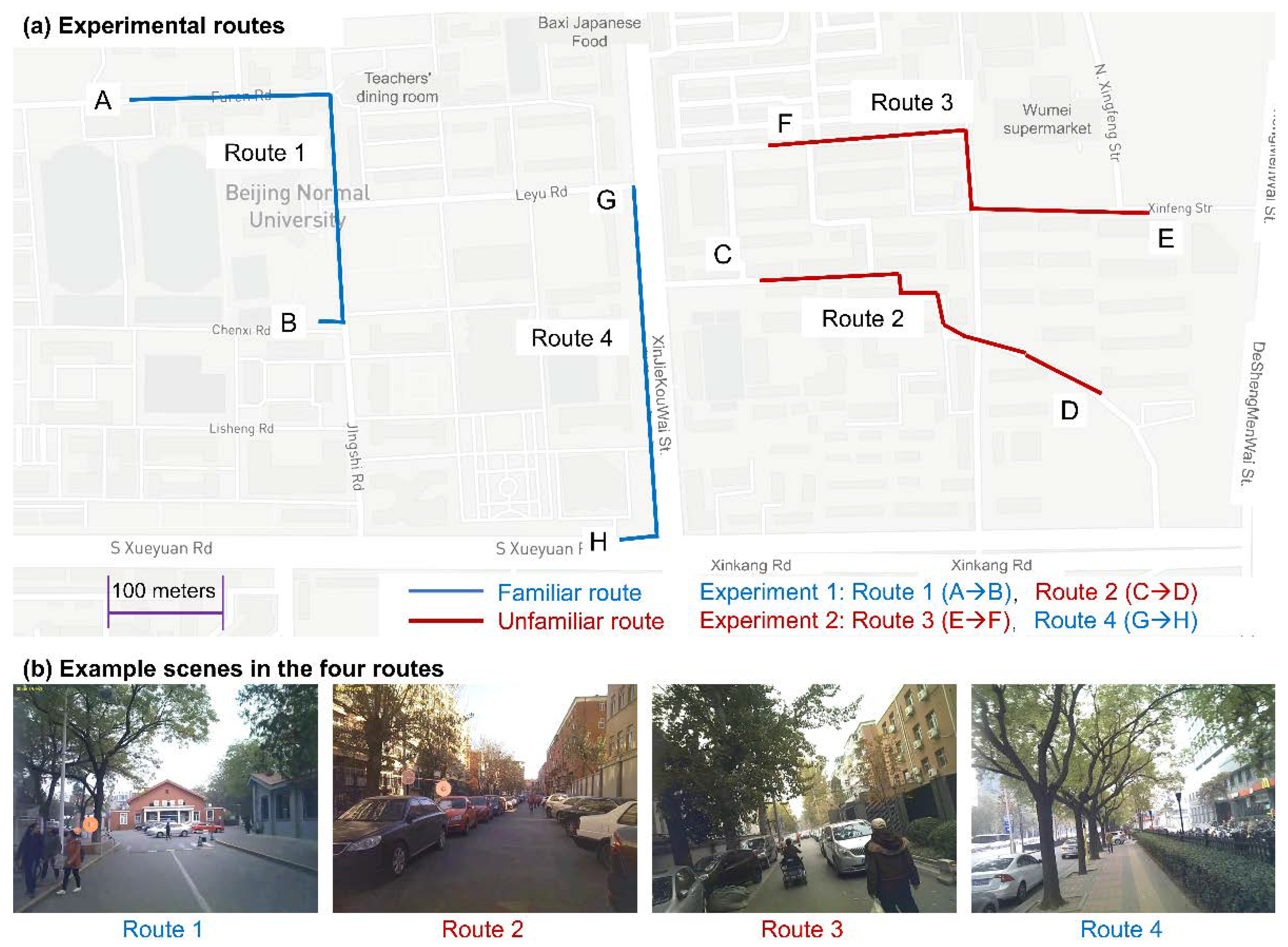
3.1. Data Collection
3.2. Data Preprocessing
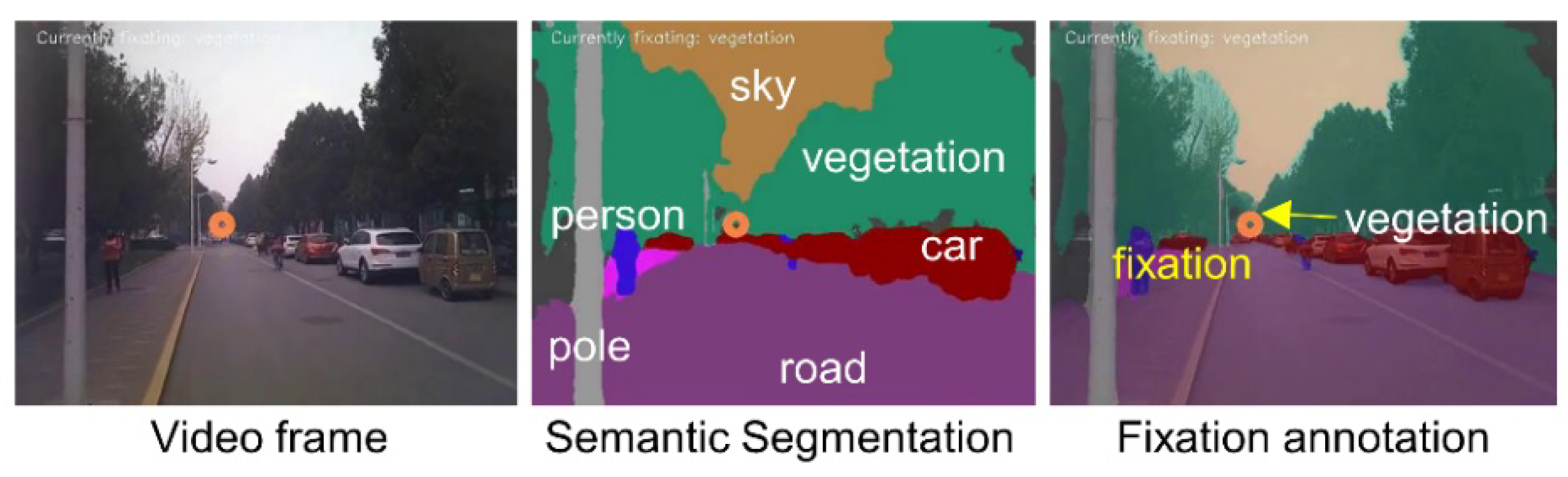
3.3. Feature Extraction
3.4. Classification and Cross-Validation
- Identification scenario. We used two cross-validation methods: a K-fold (K = 10) and a leave-one-route-out (LORO) method (Figure 6a). In the 10-fold classification, we pooled all data of the four routes and randomly split the data into 10 parts. In a round of classification, we used nine parts (e.g., Parts 1~9) of the data to train the classifier and then used the remaining part (e.g., Part 10) to test. This process was repeated until all 10 parts were tested. Unlike the K-fold classification, the LORO method first used three out of the four routes (e.g., Routes 1~3) to train the classifier and then used the remaining route (e.g., Route 4) for testing. This process was repeated until all four routes were tested. The LORO method rigorously ensured that the stimuli between the training and test data were completely different. We used the LORO method to test the generalizability of the classifier to identify subjects in new environments. In the identification scenario, for each combination of a classification method (10 rounds in 10-fold and four routes in LORO), a time window size (20 windows) and a feature set (5 feature sets plus combining all feature sets, hereafter referred to as combined features), we conducted a classification run, resulting in a total of 1800 (15 × 20 × 6) runs.
- Verification scenario. This scenario was carried out with binary classification. In a round of classification (Figure 6b), the data of a given subject acted as positive (genuine) samples (e.g., S01), and the other subjects acted as negative (impostor) samples. This was repeated until all subjects acted as genuine samples once. To avoid an imbalanced number of samples between genuine and impostor samples (impostors ≫ genuine), we randomly selected impostors to maintain balance. In a round of classification, the training and testing sets were split at a ratio of 7:3. In the verification scenario, we conducted a classification run for each combination of a subject (39 subjects), a time window size and a feature set, resulting in a total of 4680 (39 × 20 × 6) runs.
3.5. Evaluation Metrics
- Accuracy and rank-k identification rate. In the identification scenario, for a given segment (user), the classifier computes the match probability of the given segment to each candidate in the database. The biometric system then ranks the candidates based on their probabilities. There are two strategies for the system to make decisions. (1) The system uses the rank-1 (the most likely) candidate as the final predicted user. If the predicted user is true, we then consider that the system correctly identifies the segment. For all tested segments, accuracy or rank-1 identification rate (Rank-1 IR) is defined as the number of correctly identified segments divided by the total number of tested segments. (2) The system can use top-k candidates (i.e., the most likely k candidates) to predict the given segment. If the top-k candidates contain the true user, we still consider that the system correctly identifies the given segment within rank-k candidates. In other words, the system can give k tries to identify the given segment. Obviously, with the increase in k, it is easier to make a correct identification. For all tested segments, the rank-k identification rate (Rank-k IR) is the number of correctly identified segments within the top-k candidates divided by the total number of tested segments. Therefore, the accuracy, or Rank-1 IR, is a special case of Rank-k IR. The definition of the identification accuracy can be easily transferred to the verification scenario. The verification accuracy is defined as the number of correctly verified segments divided by the total number of tested segments.
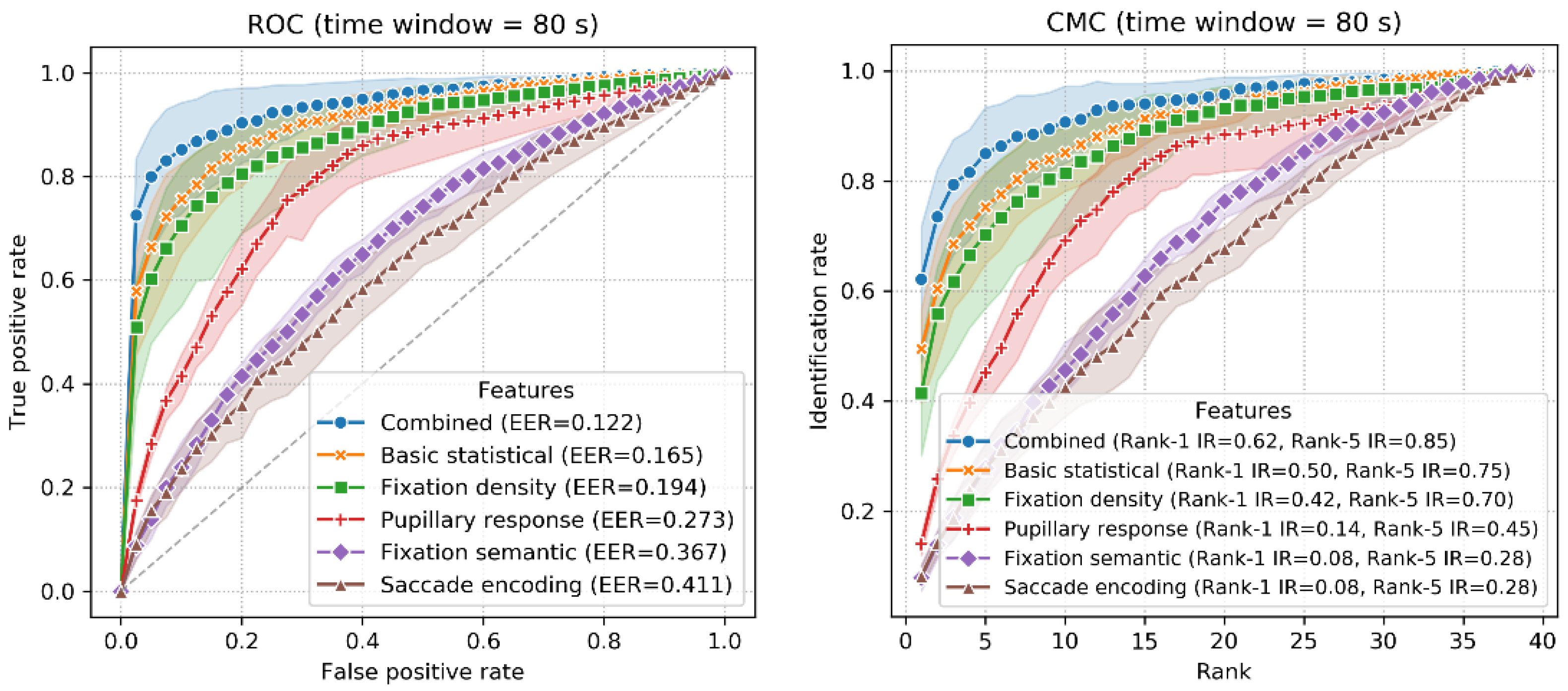
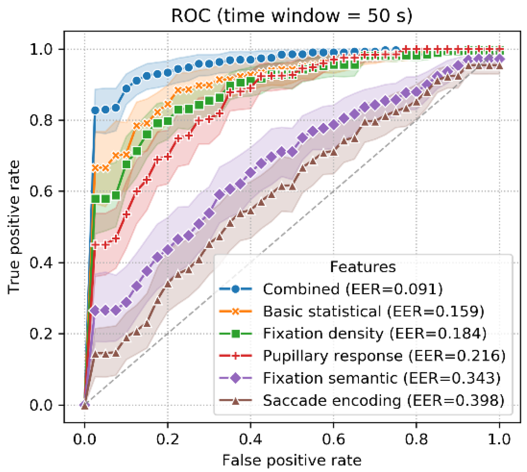
- Receiver operating characteristic (ROC) curve. The ROC curve is plotted as the true positive rate (TPR) on the y-axis versus the false positive rate (FPR) on the x-axis [61]. The equal error rate (EER) is the point where the TPR equals the FPR, indicating the possibility that a classifier misclassifies a positive segment as a negative segment or vice versa.
- Cumulative match characteristic (CMC) curve. The CMC curve is only applicable to the identification scenario. The CMC curve plots the identification rate on the y-axis for each rank (i.e., k varies from 1 to 39) on the x-axis.
4. Results
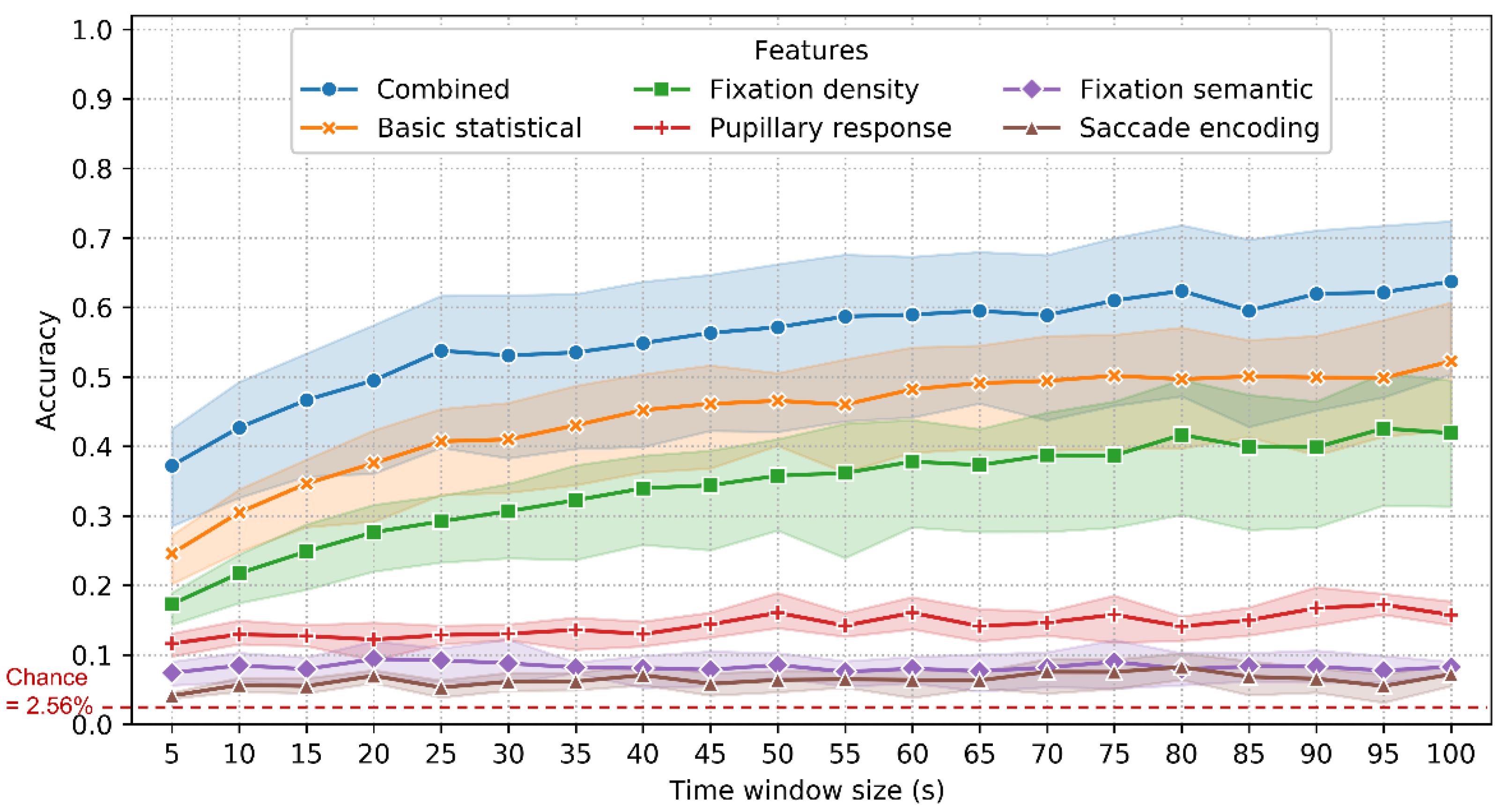
4.1. Identification Scenario: 10-Fold Classification
4.2. Identification Scenario: LORO Classification
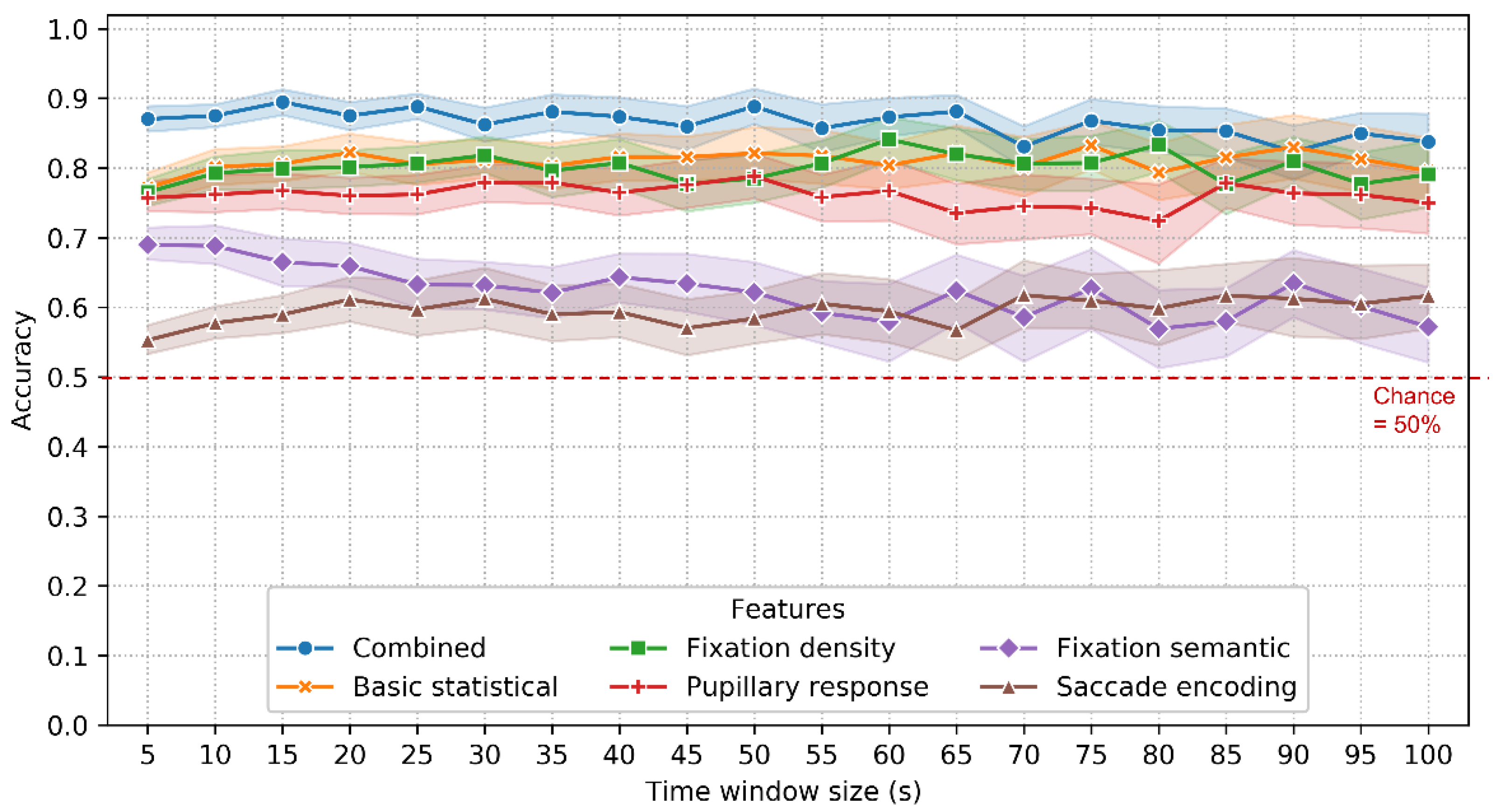
4.3. Verification Scenario
5. Discussion
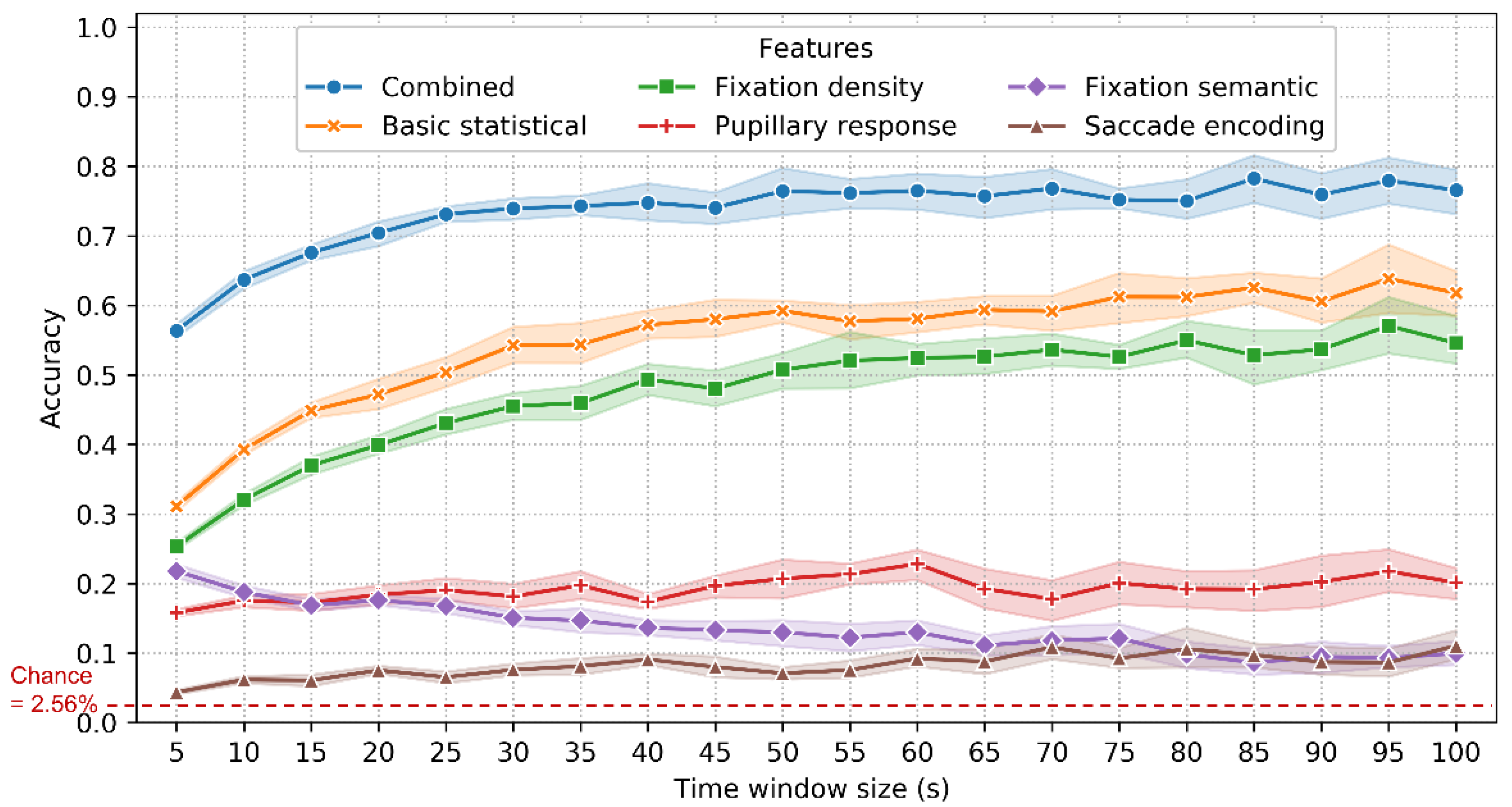
5.1. Performance, Feature Importance and Time Window Size
5.2. Reliability of Eye Movement Features
5.3. Task-Dependence of Eye Movements and Multilevel Tasks of Wayfinding
5.4. Limitations
6. Conclusions
Supplementary Materials
Author Contributions
Funding
Institutional Review Board Statement
Informed Consent Statement
Data Availability Statement
Acknowledgments
Conflicts of Interest
Appendix A

| Time Window Size (s) | Basic Statistical | Combined | Fixation Density | Pupillary Response | Saccade Encoding | Fixation Semantic |
|---|---|---|---|---|---|---|
| 5 | 0.311 | 0.564 | 0.254 | 0.158 | 0.044 | 0.218 |
| 10 | 0.393 | 0.637 | 0.321 | 0.175 | 0.062 | 0.188 |
| 15 | 0.449 | 0.676 | 0.370 | 0.173 | 0.061 | 0.169 |
| 20 | 0.472 | 0.704 | 0.399 | 0.184 | 0.075 | 0.176 |
| 25 | 0.504 | 0.731 | 0.431 | 0.191 | 0.065 | 0.168 |
| 30 | 0.542 | 0.739 | 0.455 | 0.182 | 0.076 | 0.151 |
| 35 | 0.544 | 0.743 | 0.460 | 0.197 | 0.081 | 0.147 |
| 40 | 0.572 | 0.748 | 0.494 | 0.174 | 0.091 | 0.136 |
| 45 | 0.580 | 0.741 | 0.480 | 0.197 | 0.080 | 0.133 |
| 50 | 0.592 | 0.765 | 0.507 | 0.207 | 0.071 | 0.130 |
| 55 | 0.577 | 0.762 | 0.521 | 0.214 | 0.076 | 0.122 |
| 60 | 0.581 | 0.765 | 0.524 | 0.228 | 0.092 | 0.130 |
| 65 | 0.594 | 0.757 | 0.526 | 0.193 | 0.088 | 0.111 |
| 70 | 0.591 | 0.768 | 0.536 | 0.178 | 0.109 | 0.118 |
| 75 | 0.612 | 0.752 | 0.526 | 0.201 | 0.092 | 0.121 |
| 80 | 0.612 | 0.750 | 0.550 | 0.192 | 0.106 | 0.098 |
| 85 | 0.626 | 0.783 | 0.528 | 0.192 | 0.097 | 0.086 |
| 90 | 0.606 | 0.759 | 0.537 | 0.202 | 0.087 | 0.095 |
| 95 | 0.638 | 0.780 | 0.571 | 0.218 | 0.087 | 0.093 |
| 100 | 0.618 | 0.766 | 0.546 | 0.201 | 0.111 | 0.100 |
| Time Window Size (s) | Basic Statistical | Combined | Fixation Density | Pupillary Response | Saccade Encoding | Fixation Semantic |
|---|---|---|---|---|---|---|
| 5 | 0.246 | 0.372 | 0.173 | 0.116 | 0.041 | 0.074 |
| 10 | 0.305 | 0.427 | 0.217 | 0.129 | 0.057 | 0.085 |
| 15 | 0.346 | 0.467 | 0.249 | 0.127 | 0.055 | 0.080 |
| 20 | 0.376 | 0.495 | 0.276 | 0.122 | 0.070 | 0.094 |
| 25 | 0.407 | 0.538 | 0.292 | 0.128 | 0.053 | 0.092 |
| 30 | 0.410 | 0.531 | 0.307 | 0.130 | 0.061 | 0.088 |
| 35 | 0.430 | 0.535 | 0.323 | 0.136 | 0.062 | 0.082 |
| 40 | 0.452 | 0.549 | 0.340 | 0.130 | 0.071 | 0.081 |
| 45 | 0.461 | 0.563 | 0.344 | 0.144 | 0.058 | 0.079 |
| 50 | 0.466 | 0.571 | 0.358 | 0.160 | 0.064 | 0.085 |
| 55 | 0.460 | 0.587 | 0.362 | 0.142 | 0.065 | 0.076 |
| 60 | 0.482 | 0.590 | 0.378 | 0.160 | 0.064 | 0.080 |
| 65 | 0.491 | 0.595 | 0.373 | 0.141 | 0.063 | 0.077 |
| 70 | 0.494 | 0.589 | 0.387 | 0.146 | 0.076 | 0.082 |
| 75 | 0.502 | 0.610 | 0.387 | 0.158 | 0.075 | 0.090 |
| 80 | 0.497 | 0.624 | 0.417 | 0.141 | 0.082 | 0.080 |
| 85 | 0.501 | 0.595 | 0.399 | 0.150 | 0.068 | 0.083 |
| 90 | 0.499 | 0.620 | 0.399 | 0.167 | 0.066 | 0.083 |
| 95 | 0.499 | 0.622 | 0.426 | 0.172 | 0.055 | 0.078 |
| 100 | 0.522 | 0.637 | 0.419 | 0.157 | 0.072 | 0.083 |
| Time Window Size (s) | Basic Statistical | Combined | Fixation Density | Pupillary Response | Saccade Encoding | Fixation Semantic |
|---|---|---|---|---|---|---|
| 5 | 0.772 | 0.870 | 0.765 | 0.757 | 0.553 | 0.690 |
| 10 | 0.802 | 0.875 | 0.793 | 0.762 | 0.577 | 0.688 |
| 15 | 0.806 | 0.895 | 0.799 | 0.768 | 0.590 | 0.665 |
| 20 | 0.822 | 0.875 | 0.801 | 0.760 | 0.611 | 0.659 |
| 25 | 0.806 | 0.889 | 0.807 | 0.762 | 0.597 | 0.633 |
| 30 | 0.812 | 0.862 | 0.818 | 0.779 | 0.612 | 0.632 |
| 35 | 0.803 | 0.881 | 0.796 | 0.779 | 0.590 | 0.621 |
| 40 | 0.816 | 0.874 | 0.807 | 0.765 | 0.593 | 0.643 |
| 45 | 0.816 | 0.860 | 0.777 | 0.776 | 0.570 | 0.634 |
| 50 | 0.821 | 0.889 | 0.785 | 0.788 | 0.584 | 0.622 |
| 55 | 0.818 | 0.857 | 0.807 | 0.758 | 0.605 | 0.592 |
| 60 | 0.804 | 0.873 | 0.841 | 0.767 | 0.594 | 0.579 |
| 65 | 0.821 | 0.881 | 0.820 | 0.735 | 0.567 | 0.624 |
| 70 | 0.802 | 0.831 | 0.807 | 0.745 | 0.618 | 0.586 |
| 75 | 0.833 | 0.868 | 0.807 | 0.743 | 0.609 | 0.627 |
| 80 | 0.794 | 0.854 | 0.833 | 0.724 | 0.599 | 0.569 |
| 85 | 0.815 | 0.853 | 0.777 | 0.778 | 0.617 | 0.580 |
| 90 | 0.830 | 0.823 | 0.810 | 0.764 | 0.612 | 0.635 |
| 95 | 0.813 | 0.850 | 0.777 | 0.762 | 0.605 | 0.602 |
| 100 | 0.796 | 0.838 | 0.791 | 0.750 | 0.616 | 0.572 |
References
- Jain, A.K.; Ross, A.A.; Nandakumar, K. Introduction to Biometrics; Springer: New York, NY, USA, 2011. [Google Scholar]
- Jain, A.K.; Nandakumar, K.; Ross, A. 50 years of biometric research: Accomplishments, challenges, and opportunities. Pattern Recognit. Lett. 2016, 79, 80–105. [Google Scholar] [CrossRef]
- Kasprowski, P.; Ober, J. Eye movements in biometrics. In Biometric Authentication; Maltoni, D., Jain, A.K., Eds.; Springer: Berlin/Heidelberg, Germany, 2004; pp. 248–258. [Google Scholar] [CrossRef]
- Brasil, A.R.A.; Andrade, J.O.; Komati, K.S. Eye Movements Biometrics: A Bibliometric Analysis from 2004 to 2019. Int. J. Comput. Appl. 2020, 176, 1–9. [Google Scholar] [CrossRef]
- Holland, C.; Komogortsev, O.V. Biometric identification via eye movement scanpaths in reading. In Proceedings of the 2011 International Joint Conference on Biometrics (IJCB), Washington, DC, USA, 11–13 October 2011; pp. 1–8. [Google Scholar] [CrossRef]
- Saeed, U. Eye movements during scene understanding for biometric identification. Pattern Recognit. Lett. 2016, 82, 190–195. [Google Scholar] [CrossRef]
- Kinnunen, T.; Sedlak, F.; Bednarik, R. Towards task-independent person authentication using eye movement signals. In Proceedings of the 2010 Symposium on Eye-Tracking Research & Applications, Austin, TX, USA, 22–24 March 2010; Morimoto, C.H., Istance, H., Eds.; ACM: New York, NY, USA, 2010; pp. 187–190. [Google Scholar] [CrossRef] [Green Version]
- Minh Dang, L.; Min, K.; Wang, H.; Jalil Piran, M.; Hee Lee, C.; Moon, H. Sensor-based and vision-based human activity recognition: A comprehensive survey. Pattern Recognit. 2020, 108, 107561. [Google Scholar] [CrossRef]
- Kim, S.; Billinghurst, M.; Lee, G.; Huang, W. Gaze window: A new gaze interface showing relevant content close to the gaze point. J. Soc. Inf. Disp. 2020, 28, 979–996. [Google Scholar] [CrossRef]
- Katsini, C.; Abdrabou, Y.; Raptis, G.E.; Khamis, M.; Alt, F. The role of eye gaze in security and privacy applications: Survey and future HCI research directions. In Proceedings of the 2020 CHI Conference on Human Factors in Computing Systems, Honolulu, HI, USA, 25–30 April 2020; Regina Bernhaupt, F.F.M., David, V., Josh, A., Eds.; ACM: New York, NY, USA, 2020; pp. 1–21. [Google Scholar] [CrossRef]
- Dong, W.; Qin, T.; Yang, T.; Liao, H.; Liu, B.; Meng, L.; Liu, Y. Wayfinding Behavior and Spatial Knowledge Acquisition: Are They the Same in Virtual Reality and in Real-World Environments? Ann. Am. Assoc. Geogr. 2022, 112, 226–246. [Google Scholar] [CrossRef]
- Liao, H.; Dong, W.; Huang, H.; Gartner, G.; Liu, H. Inferring user tasks in pedestrian navigation from eye movement data in real-world environments. Int. J. Geogr. Inf. Sci. 2019, 33, 739–763. [Google Scholar] [CrossRef]
- Wenczel, F.; Hepperle, L.; von Stülpnagel, R. Gaze behavior during incidental and intentional navigation in an outdoor environment. Spat. Cogn. Comput. 2017, 17, 121–142. [Google Scholar] [CrossRef] [Green Version]
- Kiefer, P.; Giannopoulos, I.; Raubal, M. Where Am I? Investigating map matching during self-localization with mobile eye tracking in an urban environment. Trans. GIS 2014, 18, 660–686. [Google Scholar] [CrossRef]
- Trefzger, M.; Blascheck, T.; Raschke, M.; Hausmann, S.; Schlegel, T. A visual comparison of gaze behavior from pedestrians and cyclists. In Proceedings of the 2018 ACM Symposium on Eye Tracking Research & Applications, Warsaw, Poland, 14–17 June 2018; p. 34. [Google Scholar]
- Liao, H.; Zhao, W.; Zhang, C.; Dong, W.; Huang, H. Detecting Individuals’ Spatial Familiarity with Urban Environments Using Eye Movement Data. Comput. Environ. Urban Syst. 2022, 93, 101758. [Google Scholar] [CrossRef]
- Abdulin, E.; Rigas, I.; Komogortsev, O. Eye Movement Biometrics on Wearable Devices: What Are the Limits? In Proceedings of the Human Factors in Computing Systems, San Jose, CA, USA, 7–12 May 2016; pp. 1503–1509. [Google Scholar]
- Tonsen, M.; Steil, J.; Sugano, Y.; Bulling, A. InvisibleEye: Mobile eye tracking using multiple low-resolution cameras and learning-based gaze estimation. In Proceedings of the ACM on Interactive, Mobile, Wearable and Ubiquitous Technologies; ACM: New York, NY, USA, 2017; Volume 1, pp. 1–21. [Google Scholar] [CrossRef]
- Schröder, C.; Zaidawi, S.M.K.A.; Prinzler, M.H.U.; Maneth, S.; Zachmann, G. Robustness of Eye Movement Biometrics Against Varying Stimuli and Varying Trajectory Length. In Proceedings of the 2020 CHI Conference on Human Factors in Computing Systems; Bernhaupt, R., Mueller, F.F., Eds.; ACM: New York, NY, USA, 2020; pp. 1–7. [Google Scholar] [CrossRef]
- Montello, D.R. Navigation. In The Cambridge Handbook of Visuospatial Thinking; Shah, P., Miyake, A., Eds.; Cambridge University Press: New York, NY, USA, 2005; pp. 257–294. [Google Scholar]
- Spiers, H.J.; Maguire, E.A. The dynamic nature of cognition during wayfinding. J. Environ. Psychol. 2008, 28, 232–249. [Google Scholar] [CrossRef] [PubMed] [Green Version]
- Komogortsev, O.V.; Jayarathna, S.; Aragon, C.R.; Mahmoud, M. Biometric identification via an oculomotor plant mathematical model. In Proceedings of the 2010 Symposium on Eye-Tracking Research and Applications, Austin, TX, USA, 22–24 March 2010; pp. 57–60. [Google Scholar]
- Holland, C.D.; Komogortsev, O.V. Complex Eye Movement Pattern Biometrics: The Effects of Environment and Stimulus. IEEE Trans. Inf. Forensics Secur. 2013, 8, 2115–2126. [Google Scholar] [CrossRef]
- Rigas, I.; Abdulin, E.; Komogortsev, O. Towards a multi-source fusion approach for eye movement-driven recognition. Inf. Fusion 2016, 32, 13–25. [Google Scholar] [CrossRef] [Green Version]
- Bednarik, R.; Kinnunen, T.; Mihaila, A.; Fränti, P. Eye-movements as a biometric. In SCIA: Scandinavian Conference on Image Analysis; Kalviainen, H., Parkkinen, J., Kaarna, A., Eds.; Springer: Berlin/Heidelberg, Germany, 2005; pp. 780–789. [Google Scholar] [CrossRef] [Green Version]
- Rigas, I.; Economou, G.; Fotopoulos, S. Biometric identification based on the eye movements and graph matching techniques. Pattern Recognit. Lett. 2012, 33, 786–792. [Google Scholar] [CrossRef]
- Cantoni, V.; Galdi, C.; Nappi, M.; Porta, M.; Riccio, D. GANT: Gaze analysis technique for human identification. Pattern Recognit. 2015, 48, 1027–1038. [Google Scholar] [CrossRef]
- Rigas, I.; Komogortsev, O. Biometric recognition via fixation density maps. In Proceedings of the SPIE Defense + Security, Baltimore, MD, USA, 25 May 2016; Available online: https://userweb.cs.txstate.edu/~ok11/papers_published/2014_DDS_Ri_Ko.pdf (accessed on 9 April 2022).
- Liao, H.; Dong, W.; Zhan, Z. Identifying Map Users with Eye Movement Data from Map-Based Spatial Tasks: User Privacy Concerns. Cartogr. Geogr. Inf. Sci. 2022, 49, 50–69. [Google Scholar] [CrossRef]
- Rigas, I.; Komogortsev, O.V. Current research in eye movement biometrics: An analysis based on BioEye 2015 competition. Image Vis. Comput. 2017, 58, 129–141. [Google Scholar] [CrossRef] [Green Version]
- DELL. Alienware m17 Gaming Laptop with Tobii Eye Tracking. Available online: https://www.dell.com/en-us/shop/dell-laptops/alienware-m17-r2-gaming-laptop/spd/alienware-m17-r2-laptop (accessed on 19 May 2021).
- HTC. VIVE Pro Eye Office. Available online: https://business.vive.com/us/product/vive-pro-eye-office/ (accessed on 15 May 2021).
- Microsoft. HoloLens 2 A New Reality for Computing: See New Ways to Work Better Together with the Ultimate Mixed Reality Device. Available online: https://www.microsoft.com/en-us/hololens (accessed on 13 December 2020).
- BMW. BMW Camera Keeps an Eye on the Driver. Available online: https://www.autonews.com/article/20181001/OEM06/181009966/bmw-camera-keeps-an-eye-on-the-driver (accessed on 22 January 2022).
- Chuang, L.L.; Duchowski, A.T.; Qvarfordt, P.; Weiskopf, D. Ubiquitous Gaze Sensing and Interaction (Dagstuhl Seminar 18252). Available online: https://www.dagstuhl.de/de/programm/kalender/semhp/?semnr=18252 (accessed on 22 July 2021).
- Sim, T.; Zhang, S.; Janakiraman, R.; Kumar, S. Continuous verification using multimodal biometrics. IEEE Trans. Pattern Anal. Mach. Intell. 2007, 29, 687–700. [Google Scholar] [CrossRef]
- Liao, H.; Dong, W. Challenges of Using Eye Tracking to Evaluate Usability of Mobile Maps in Real Environments. Available online: https://use.icaci.org/wp-content/uploads/2018/11/LiaoDong.pdf (accessed on 1 February 2020).
- Tobii. Pro Glasses 3 Product Description. Available online: https://www.tobiipro.com/siteassets/tobii-pro/product-descriptions/product-description-tobii-pro-glasses-3.pdf/?v=1.7 (accessed on 27 February 2022).
- SMI. BeGaze Manual Version 3.7. Available online: www.humre.vu.lt/files/doc/Instrukcijos/SMI/BeGaze2.pdf (accessed on 9 June 2018).
- Tobii. Tobii Pro Spectrum Product Description. Available online: https://www.tobiipro.com/siteassets/tobii-pro/product-descriptions/tobii-pro-spectrum-product-description.pdf/?v=2.2 (accessed on 27 February 2022).
- SR Research. EyeLink 1000 Plus—The Most Flexible Eye Tracker—SR Research. Available online: https://www.sr-research.com/eyelink-1000-plus/ (accessed on 22 March 2022).
- Salvucci, D.D.; Goldberg, J.H. Identifying fixations and saccades in eye-tracking protocols. In Proceedings of the 2000 Symposium on Eye Tracking Research & Applications, Palm Beach Gardens, FL, USA, 6–8 November 2000; Duchowski, A.T., Ed.; ACM: New York, NY, USA, 2000; pp. 71–78. [Google Scholar]
- Bayat, A.; Pomplun, M. Biometric identification through eye-movement patterns. In Advances in Human Factors in Simulation and Modeling, Advances in Intelligent Systems and Computing 591; Cassenti, D.N., Ed.; Springer International Publishing: Cham, Switzerland, 2017; pp. 583–594. [Google Scholar] [CrossRef]
- Van der Wel, P.; van Steenbergen, H. Pupil dilation as an index of effort in cognitive control tasks: A review. Psychon. Bull. Rev. 2018, 25, 2005–2015. [Google Scholar] [CrossRef]
- Beatty, J. Task-evoked pupillary responses, processing load, and the structure of processing resources. Psychol. Bull. 1982, 91, 276–292. [Google Scholar] [CrossRef]
- Liao, H.; Dong, W.; Peng, C.; Liu, H. Exploring differences of visual attention in pedestrian navigation when using 2D maps and 3D geo-browsers. Cartogr. Geogr. Inf. Sci. 2017, 44, 474–490. [Google Scholar] [CrossRef]
- Darwish, A.; Pasquier, M. Biometric identification using the dynamic features of the eyes. In Proceedings of the 2013 IEEE Sixth International Conference on Biometrics: Theory, Applications and Systems (BTAS), Arlington, VA, USA, 29 September–2 October 2013; pp. 1–6. [Google Scholar]
- Rigas, I.; Komogortsev, O.V. Biometric recognition via probabilistic spatial projection of eye movement trajectories in dynamic visual environments. IEEE Trans. Inf. Forensics Secur. 2014, 9, 1743–1754. [Google Scholar] [CrossRef]
- Andrienko, G.; Andrienko, N.; Burch, M.; Weiskopf, D. Visual analytics methodology for eye movement studies. IEEE Trans. Vis. Comput. Graph. 2012, 18, 2889–2898. [Google Scholar] [CrossRef] [PubMed] [Green Version]
- Ooms, K.; De Maeyer, P.; Fack, V.; Van Assche, E.; Witlox, F. Interpreting maps through the eyes of expert and novice users. Int. J. Geogr. Inf. Sci. 2012, 26, 1773–1788. [Google Scholar] [CrossRef]
- Chen, L.-C.; Zhu, Y.; Papandreou, G.; Schroff, F.; Adam, H. Encoder-decoder with atrous separable convolution for semantic image segmentation. arXiv 2018, arXiv:1802.02611. [Google Scholar]
- Cordts, M.; Omran, M.; Ramos, S.; Rehfeld, T.; Enzweiler, M.; Benenson, R.; Franke, U.; Roth, S.; Schiele, B. The cityscapes dataset for semantic urban scene understanding. In Proceedings of the IEEE Conference on Computer Vision and Pattern Recognition, Las Vegas, NV, USA, 27–30 June 2016; pp. 3213–3223. [Google Scholar]
- Dong, W.; Liao, H.; Liu, B.; Zhan, Z.; Liu, H.; Meng, L.; Liu, Y. Comparing pedestrians’ gaze behavior in desktop and in real environments. Cartogr. Geogr. Inf. Sci. 2020, 47, 432–451. [Google Scholar] [CrossRef]
- Lowe, D.G. Distinctive Image Features from Scale-Invariant Keypoints. Int. J. Comput. Vis. 2004, 60, 91–110. [Google Scholar] [CrossRef]
- Bulling, A.; Ward, J.A.; Gellersen, H.; Troster, G. Eye movement analysis for activity recognition using electrooculography. IEEE Trans. Pattern Anal. Mach. Intell. 2011, 33, 741–753. [Google Scholar] [CrossRef]
- Breiman, L. Random forests. Mach. Learn. 2001, 45, 5–32. [Google Scholar] [CrossRef] [Green Version]
- Cutler, A.; Cutler, D.R.; Stevens, J.R. Random forests. In Ensemble Machine Learning: Methods and Applications; Zhang, C., Ma, Y., Eds.; Springer: Boston, MA, USA, 2012; pp. 157–175. [Google Scholar] [CrossRef]
- Kasprowski, P. The impact of temporal proximity between samples on eye movement biometric identification. In IFIP International Conference on Computer Information Systems and Industrial Management; Saeed, K., Chaki, R., Cortesi, A., Wierzchoń, S., Eds.; Springer: Berlin/Heidelberg, Germany, 2013; pp. 77–87. [Google Scholar] [CrossRef] [Green Version]
- Kasprowski, P.; Rigas, I. The influence of dataset quality on the results of behavioral biometric experiments. In Proceedings of the 2013 International Conference of the BIOSIG Special Interest Group (BIOSIG), Darmstadt, Germany, 5–6 September 2013; Brömme, A., Busch, C., Eds.; IEEE: Piscataway, NJ, USA, 2013; pp. 1–8. [Google Scholar]
- Pedregosa, F.; Varoquaux, G.; Gramfort, A.; Michel, V.; Thirion, B.; Grisel, O.; Blondel, M.; Prettenhofer, P.; Weiss, R.; Dubourg, V.; et al. Scikit-learn: Machine Learning in Python. J. Mach. Learn. Res. 2011, 12, 2825–2830. [Google Scholar]
- Fawcett, T. An introduction to ROC analysis. Pattern Recognit. Lett. 2006, 27, 861–874. [Google Scholar] [CrossRef]
- Liang, Z.; Tan, F.; Chi, Z. Video-based biometric identification using eye tracking technique. In Proceedings of the 2012 IEEE International Conference on Signal Processing, Communication and Computing (ICSPCC 2012), Hong Kong, China, 12–15 August 2012; Lam, K.K.M., Huang, J., Eds.; IEEE: Piscataway, NJ, USA, 2012; pp. 728–733. [Google Scholar] [CrossRef]
- Klein, C.; Fischer, B. Instrumental and test–retest reliability of saccadic measures. Biol. Psychol. 2005, 68, 201–213. [Google Scholar] [CrossRef] [PubMed]
- Marandi, R.Z.; Madeleine, P.; Omland, Ø.; Vuillerme, N.; Samani, A. Reliability of oculometrics during a mentally demanding task in young and old adults. IEEE Access 2018, 6, 17500–17517. [Google Scholar] [CrossRef]
- Bargary, G.; Bosten, J.M.; Goodbourn, P.T.; Lawrance-Owen, A.J.; Hogg, R.E.; Mollon, J.D. Individual differences in human eye movements: An oculomotor signature? Vis. Res. 2017, 141, 157–169. [Google Scholar] [CrossRef] [PubMed]
- Vikesdal, G.H.; Langaas, T. Saccade latency and fixation stability: Repeatability and reliability. J. Eye Mov. Res. 2016, 9, 1–13. [Google Scholar]
- Ettinger, U.; Kumari, V.; Crawford, T.J.; Davis, R.E.; Sharma, T.; Corr, P.J. Reliability of smooth pursuit, fixation, and saccadic eye movements. Psychophysiology 2003, 40, 620–628. [Google Scholar] [CrossRef]
- Delikostidis, I.; van Elzakker, C.P.; Kraak, M.-J. Overcoming challenges in developing more usable pedestrian navigation systems. Cartogr. Geogr. Inf. Sci. 2015, 43, 189–207. [Google Scholar] [CrossRef]
- Borji, A.; Itti, L. Defending Yarbus: Eye movements reveal observers’ task. J. Vis. 2014, 14, 1–12. [Google Scholar] [CrossRef]
- Boisvert, J.F.G.; Bruce, N.D.B. Predicting task from eye movements: On the importance of spatial distribution, dynamics, and image features. Neurocomputing 2016, 207, 653–668. [Google Scholar] [CrossRef]
- Yarbus, A.L. Eye Movements and Vision; Plenum Press: New York, NY, USA, 1967; Volume 2. [Google Scholar]


| Route | Mean Duration (s) | SD | Number of Recordings |
|---|---|---|---|
| Route 1 | 361.48 | 48.79 | 38 |
| Route 2 | 396.21 | 59.51 | 37 |
| Route 3 | 527.33 | 121.75 | 38 |
| Route 4 | 384.19 | 59.77 | 33 |
| Overall | 418.58 | 102.02 | 146 |
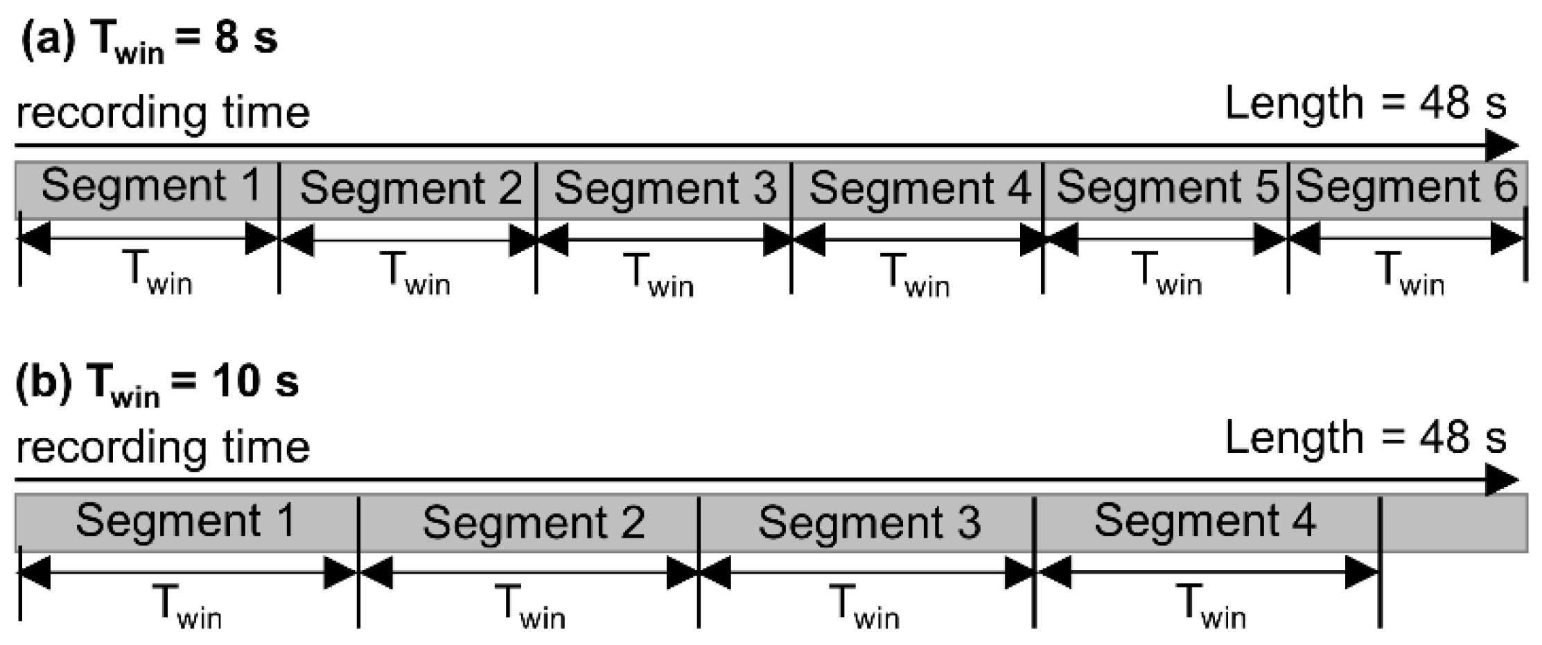
| Twin (s) | 5 | 10 | 15 | 20 | 25 | 30 | 35 | 40 | 45 | 50 | 55 | 60 | 65 | 70 | 75 | 80 | 85 | 90 | 95 | 100 |
|---|---|---|---|---|---|---|---|---|---|---|---|---|---|---|---|---|---|---|---|---|
| Segment count | 11974 | 6101 | 4110 | 3102 | 2503 | 2098 | 1793 | 1570 | 1403 | 1270 | 1166 | 1064 | 992 | 923 | 867 | 822 | 772 | 736 | 694 | 670 |
| Eye Movement Metric | Statistic | N | |
|---|---|---|---|
| Fixation | Fixation duration, fixation dispersion | mean, standard deviation, median, max, min, 1/4 quantile, 3/4 quantile and skewness | 16 |
| Saccade | saccade duration, saccade amplitude, saccade velocity, saccade latency, saccade acceleration, saccade acceleration peak, saccade deceleration peak and saccade velocity peak | 64 | |
| Blink | blink duration | 8 | |
| Fixation frequency, saccade frequency, blink frequency, scanpath convex hull area and scanpath length | 5 | ||
| Subject ID | Route | Window Size | Segment ID | FC- Building | FC- Map | FC- Person | FC- Road | FD- Building | FD- Map | FD- Person | FD-Road |
|---|---|---|---|---|---|---|---|---|---|---|---|
| S01 | Route 1 | 50 | 1 | 9 | 0 | 4 | 23 | 1365 | 0 | 1531 | 5108 |
| S01 | Route 1 | 50 | 2 | 3 | 0 | 0 | 18 | 815 | 0 | 0 | 3795 |
| S01 | Route 1 | 50 | 3 | 17 | 0 | 1 | 33 | 3478 | 0 | 167 | 8400 |
| S01 | Route 1 | 50 | 4 | 8 | 0 | 11 | 19 | 1448 | 0 | 2380 | 3212 |
| S01 | Route 1 | 50 | 5 | 2 | 0 | 0 | 31 | 333 | 0 | 0 | 6040 |
Publisher’s Note: MDPI stays neutral with regard to jurisdictional claims in published maps and institutional affiliations. |
© 2022 by the authors. Licensee MDPI, Basel, Switzerland. This article is an open access article distributed under the terms and conditions of the Creative Commons Attribution (CC BY) license (https://creativecommons.org/licenses/by/4.0/).
Share and Cite
Liao, H.; Zhao, W.; Zhang, C.; Dong, W. Exploring Eye Movement Biometrics in Real-World Activities: A Case Study of Wayfinding. Sensors 2022, 22, 2949. https://doi.org/10.3390/s22082949
Liao H, Zhao W, Zhang C, Dong W. Exploring Eye Movement Biometrics in Real-World Activities: A Case Study of Wayfinding. Sensors. 2022; 22(8):2949. https://doi.org/10.3390/s22082949
Chicago/Turabian StyleLiao, Hua, Wendi Zhao, Changbo Zhang, and Weihua Dong. 2022. "Exploring Eye Movement Biometrics in Real-World Activities: A Case Study of Wayfinding" Sensors 22, no. 8: 2949. https://doi.org/10.3390/s22082949
APA StyleLiao, H., Zhao, W., Zhang, C., & Dong, W. (2022). Exploring Eye Movement Biometrics in Real-World Activities: A Case Study of Wayfinding. Sensors, 22(8), 2949. https://doi.org/10.3390/s22082949