Author Contributions
Conceptualization, H.A.B., C.S., M.P., P.L. and E.P.; data curation, J.E.R., P.L. and E.P.; formal analysis, H.A.B.; funding acquisition, E.P.; investigation, H.A.B., C.S., P.L. and E.P.; methodology, H.A.B., P.L. and E.P.; project administration, J.E.R., P.L. and E.P.; resources, E.P.; software, H.A.B.; supervision, C.S., M.P., P.L. and E.P.; validation, H.A.B., C.S., P.L. and E.P.; visualization, H.A.B.; writing—original draft, H.A.B.; writing—review and editing, H.A.B., C.S., M.P., P.L. and E.P. All authors have read and agreed to the published version of the manuscript.
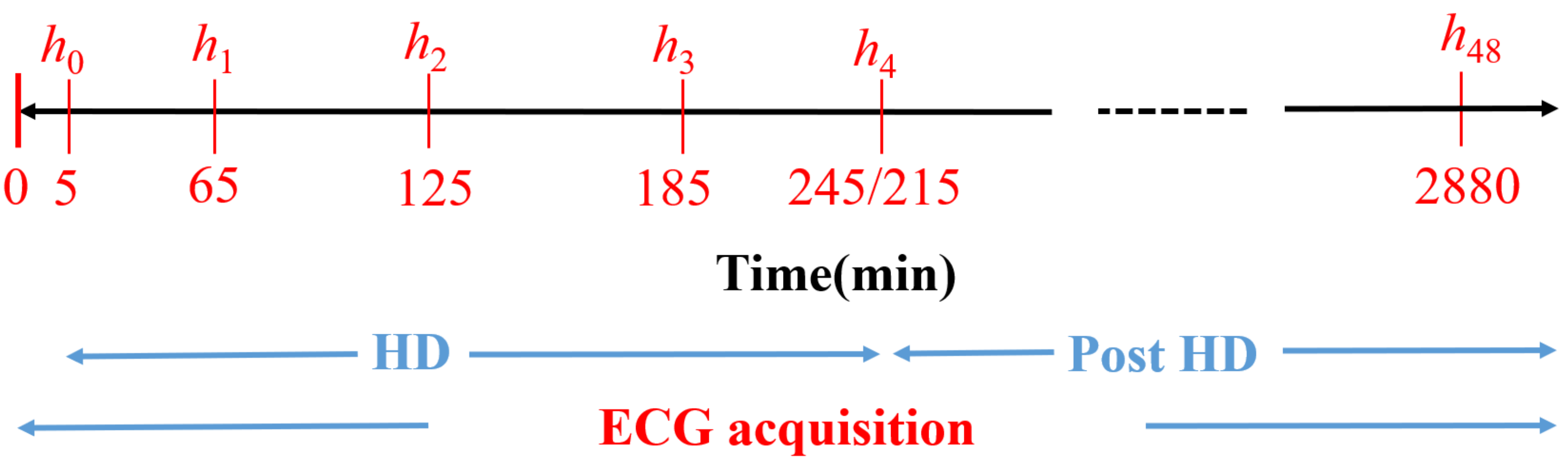
Figure 1.
Diagram of the study protocol. to are the time points (in minutes) for blood sample extraction. Reproduced with permission from Bukhari et al., Computers in Biology and Medicine; published by Elsevier, 2022.
Figure 1.
Diagram of the study protocol. to are the time points (in minutes) for blood sample extraction. Reproduced with permission from Bukhari et al., Computers in Biology and Medicine; published by Elsevier, 2022.
Figure 2.
Flow chart showing the ECG processing steps performed in this study, from the collection of raw ECGs to the estimation of and .
Figure 2.
Flow chart showing the ECG processing steps performed in this study, from the collection of raw ECGs to the estimation of and .
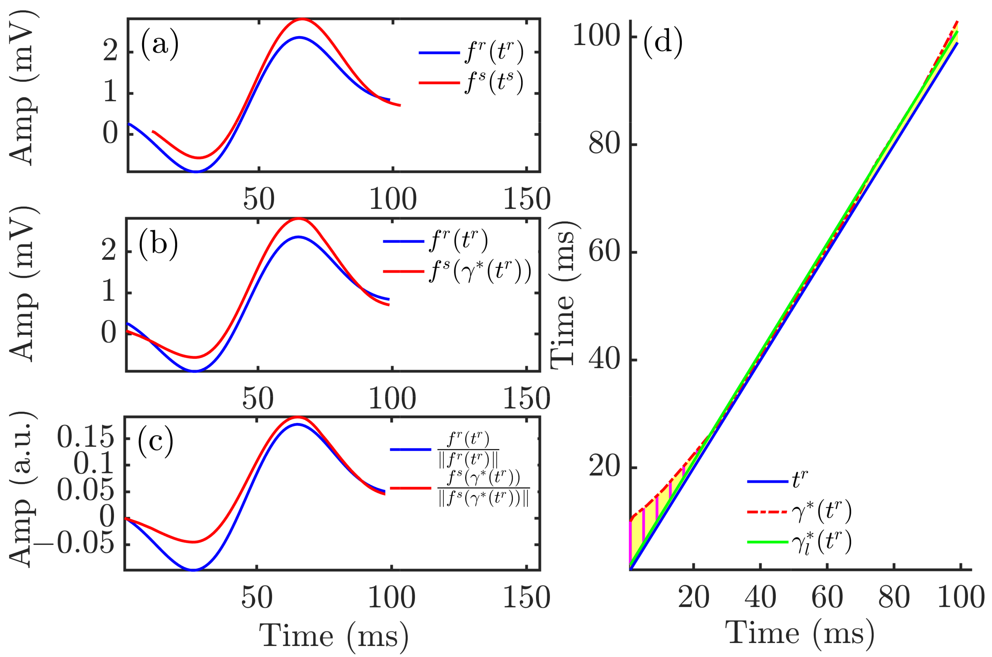
Figure 3.
Time warping of QRS complexes. Panel (a) shows the reference (blue) and investigated (red) QRS complexes obtained from an ECG segment during HD. Panel (b) shows the warped QRS complexes, which had the same duration whilst keeping the original amplitude. Panel (c) depicts the warped QRS complexes after normalization by their L2-norms. The yellow area in panel (d) represents , which quantified the total amount of warping. The green solid line is the linear regression function best fitted to .
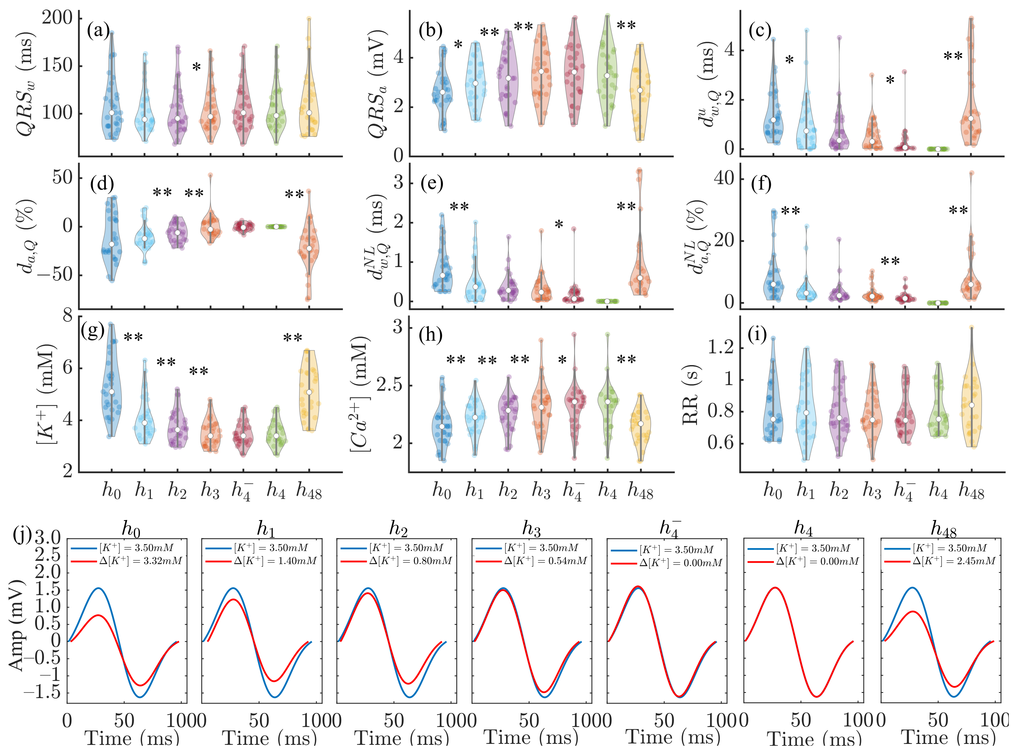
Figure 4.
Panels (a–f): changes in , , , , and during HD stages. Panels (g–i): corresponding variations in , and RR. In panels (a–i), * denotes and ** denotes . In each panel, the central white dot indicates the median. Each dot corresponds to an individual patient. Panel (j): MWQRS (red) of a patient at different HD stages and reference MWQRS (blue). denotes the change in with respect to the end of HD ().
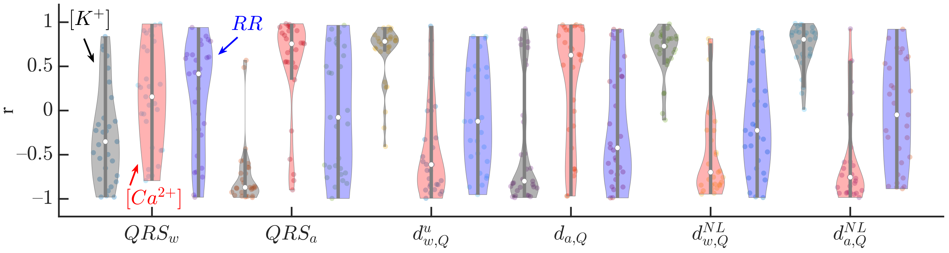
Figure 5.
Pearson correlation coefficients between QRS markers (, , , , and ) and (black), (red) and RR (blue) for all patients at all HD points. The central white dot indicates the median. Each dot corresponds to an individual patient.
Figure 5.
Pearson correlation coefficients between QRS markers (, , , , and ) and (black), (red) and RR (blue) for all patients at all HD points. The central white dot indicates the median. Each dot corresponds to an individual patient.
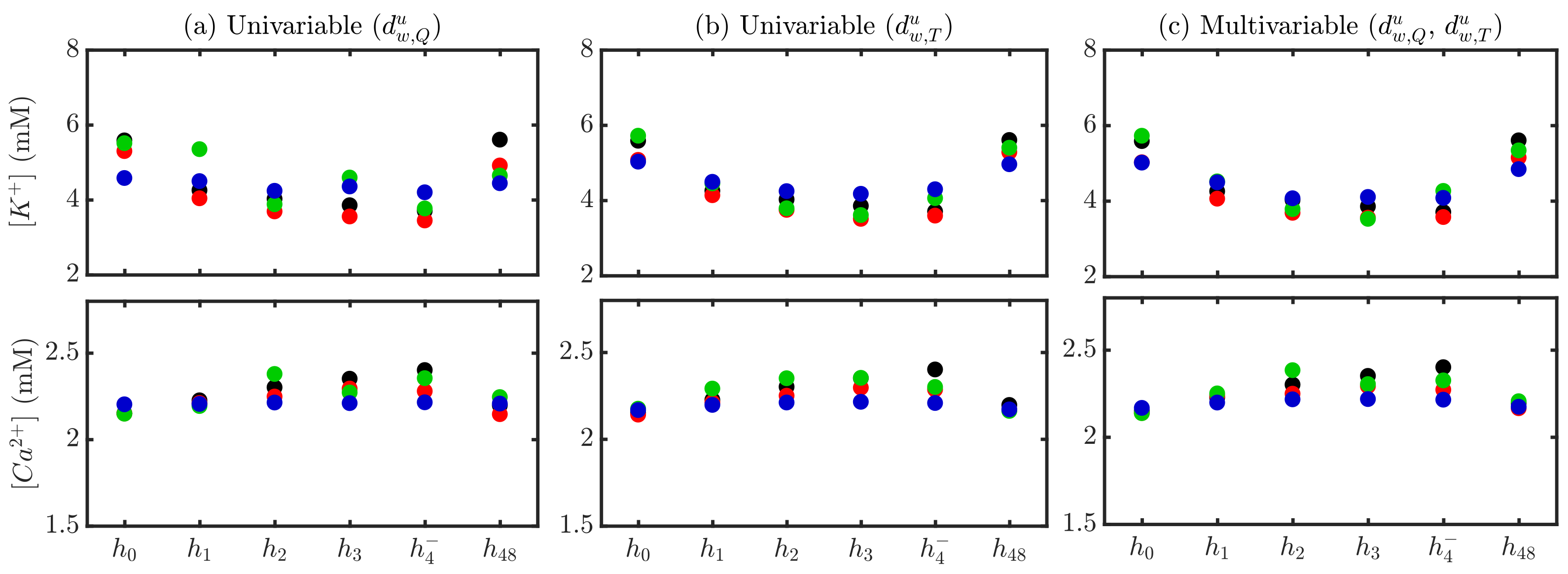
Figure 6.
Actual (black) and estimated and for a patient using stage-specific (red), patient-specific (green) and global (blue) approaches. Univariable -based estimation is shown in (panel a), -based in (panel b) and multivariable - -based in (panel c).
Figure 6.
Actual (black) and estimated and for a patient using stage-specific (red), patient-specific (green) and global (blue) approaches. Univariable -based estimation is shown in (panel a), -based in (panel b) and multivariable - -based in (panel c).
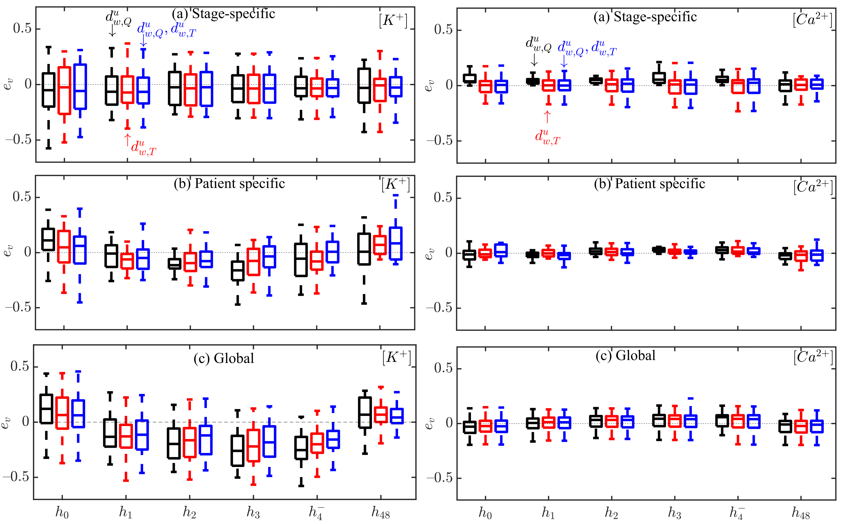
Figure 7.
Box plots of and estimation errors during HD stages for all patients using (black), (red) and the combination of and (blue) for stage-specific (top), patient-specific (middle) and global (bottom) approaches. The central line indicates the median, whereas top and bottom edges show the 25th and 75th percentiles.
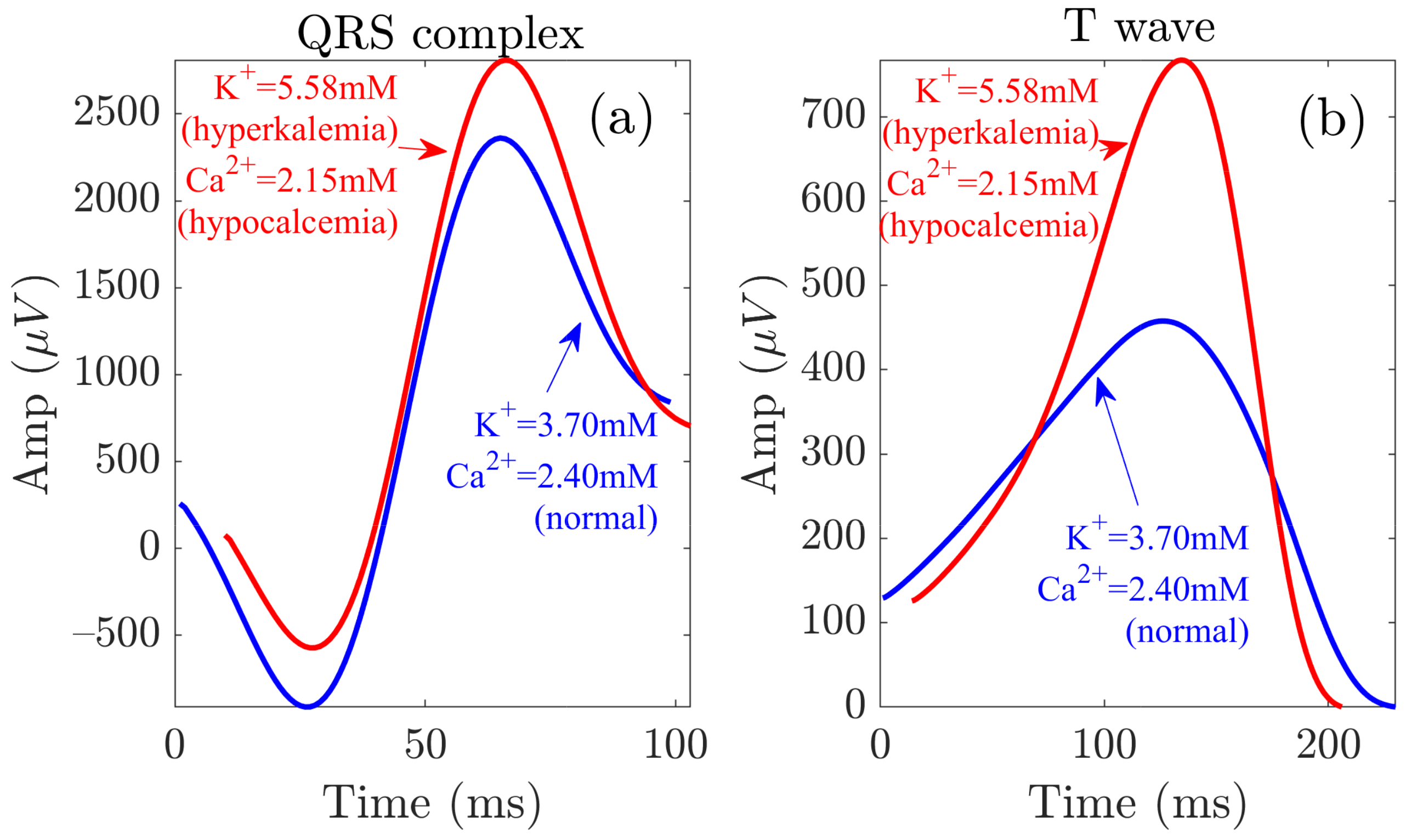
Figure 8.
QRS and T wave variations at the start (red) and end (blue) of the HD session. Panels (a,b) show the waveforms related to the QRS complex and the T wave, respectively.
Figure 8.
QRS and T wave variations at the start (red) and end (blue) of the HD session. Panels (a,b) show the waveforms related to the QRS complex and the T wave, respectively.
Table 1.
Characteristics of the study population. Values are expressed as number (%) for categorical variables and median (interquartile range, IQR) for continuous variables. Reproduced with permission from Bukhari et al., Computers in Biology and Medicine; published by Elsevier, 2022.
Table 1.
Characteristics of the study population. Values are expressed as number (%) for categorical variables and median (interquartile range, IQR) for continuous variables. Reproduced with permission from Bukhari et al., Computers in Biology and Medicine; published by Elsevier, 2022.
| Characteristics | Quantity |
|---|
| Age [years] | |
| Gender [male/female] | 20 (69%)/9 (31%) |
| Electrolyte concentrations | |
| [Pre HD] (mM) | |
| [End HD] (mM) | |
| [Pre HD] (mM) | |
| [End HD] (mM) | |
| | #Patients (%) |
| HD session duration | |
| 240 min | |
| 210 min | |
| Dialysate composition | |
| Potassium (1.5 mM) | |
| Potassium (3 mM) | |
| Potassium (variable mM) | |
| Calcium (0.75 mM) | |
| Calcium (0.63 mM) | |
Table 2.
p-values from the parametric test (t-test) to evaluate statistical significance of non-zero mean Fisher z-transformed Pearson correlation coefficients between QRS markers and , and RR.
Table 2.
p-values from the parametric test (t-test) to evaluate statistical significance of non-zero mean Fisher z-transformed Pearson correlation coefficients between QRS markers and , and RR.
| p-Values | | | | | | |
|---|
| | 0.01
| 0.01
| 0.01
| 0.01
| 0.01
|
| | 0.01
| 0.01
| | 0.01
| 0.01
|
| | | | | | |
Table 3.
Actual and estimated and values over the study population at each HD stage using multivariable (m) estimation and stage-specific (S), patient-specific (P) and global (G) approaches. Values are expressed as median (IQR) and the units are mM.
Table 3.
Actual and estimated and values over the study population at each HD stage using multivariable (m) estimation and stage-specific (S), patient-specific (P) and global (G) approaches. Values are expressed as median (IQR) and the units are mM.
| Actual vs. Estimated | | | | | | |
|---|
| 5.10 (1.30) | 3.90 (0.86) | 3.64 (0.81) | 3.40 (0.71) | 3.40 (0.56) | 5.08 (1.53) |
| 5.31 (0.43) | 4.03 (0.18) | 3.70 (0.08) | 3.49 (0.09) | 3.43 (0.05) | 4.56 (1.21) |
| 4.76 (1.90) | 4.01 (1.33) | 3.84 (1.16) | 3.46 (0.97) | 3.28 (0.44) | 4.43 (1.46) |
| 4.50 (0.71) | 4.33 (0.40) | 4.07 (0.33) | 3.97 (0.26) | 3.84 (0.19) | 4.57 (0.75) |
| 2.15 (0.20) | 2.23 (0.20) | 2.29 (0.19) | 2.31 (0.23) | 2.36 (0.21) | 2.17 (0.20) |
| 2.13 (0.02) | 2.21 (0.05) | 2.25 (0.02) | 2.31 (0.05) | 2.28 (0.03) | 2.07 (0.13) |
| 2.06 (0.29) | 2.27 (0.23) | 2.21 (0.26) | 2.29 (0.20) | 2.25 (0.23) | 2.18 (0.20) |
| 2.19 (0.04) | 2.20 (0.02) | 2.22 (0.02) | 2.23 (0.01) | 2.23 (0.01) | 2.19 (0.04) |
Table 4.
Intra-patient Pearson correlation coefficient r between actual and estimated using univariable and multivariable estimators, with stage-specific (S), patient-specific (P) and global (G) approaches. Values are expressed as median (IQR).
Table 4.
Intra-patient Pearson correlation coefficient r between actual and estimated using univariable and multivariable estimators, with stage-specific (S), patient-specific (P) and global (G) approaches. Values are expressed as median (IQR).
| | | , |
|---|
| S | 0.98 (0.08) | 0.96 (0.06) | 0.93 (0.30) |
| P | 0.56 (0.75) | 0.55 (0.90) | 0.75 (0.51) |
| G | 0.75 (0.15) | 0.82 (0.35) | 0.86 (0.32) |
Table 5.
Intra-patient Pearson correlation coefficient r between actual and estimated using univariable and multivariable estimators, with stage-specific (S), patient-specific (P) and global (G) approaches. Values are expressed as median (IQR).
Table 5.
Intra-patient Pearson correlation coefficient r between actual and estimated using univariable and multivariable estimators, with stage-specific (S), patient-specific (P) and global (G) approaches. Values are expressed as median (IQR).
| | | , |
| S | 0.88 (0.38) | 0.88 (0.22) | 0.80 (0.78) |
| P | 0.88 (0.22) | 0.63 (0.59) | 0.63 (0.37) |
| G | 0.64 (0.73) | 0.64 (0.49) | 0.70 (0.55) |
Table 6.
Estimation errors (e) using stage-specific (S), patient-specific (P) and global (G) approach-based estimators, from all patients at all HD time points. Values are expressed as mean ± standard deviation and the units are mM.
Table 6.
Estimation errors (e) using stage-specific (S), patient-specific (P) and global (G) approach-based estimators, from all patients at all HD time points. Values are expressed as mean ± standard deviation and the units are mM.
| e |
S
|
P
|
G
|
|---|
| | | |
| | | |
| | | |
| | | |
| and | | | |
Table 7.
Estimation errors (e) using stage-specific (S), patient-specific (P) and global (G) approach-based estimators, from all patients at all HD time points. Values are expressed as mean ± standard deviation and the units are mM.
Table 7.
Estimation errors (e) using stage-specific (S), patient-specific (P) and global (G) approach-based estimators, from all patients at all HD time points. Values are expressed as mean ± standard deviation and the units are mM.
| e |
S
|
P
|
G
|
|---|
| | | |
| | | |
| | | |
| | | |
| and | | | |


 ,
, 


