1. Introduction
Since the mid-1980s, remarkable research efforts and investments have been devoted to developing autonomous driving technology [
1,
2]. Automotive companies have dedicated remarkable efforts to the commercialization of this technology, which requires near-perfect safety conditions [
3,
4,
5]. Therefore, precise real-time perception of the surrounding environment using various sensors, such as a global navigation satellite system (GNSS), cameras, light detection and ranging (LiDAR) equipment, radio detection and ranging (RADAR) technology, and the inertial measurement unit (IMU), is essential [
6]. Diverse types of information are required for safe autonomous driving, including the location of the ego vehicle, road environment, and spatial relationship between the surrounding objects. The techniques used for extracting such information from the environment are interdependent. In addition, as most perception methods are performed under the assumption that the pose of the ego vehicle is accurately known, inaccurate pose information may result in the deterioration of the performance of the autonomous driving system. Although accurate information regarding the position of a vehicle can be obtained using GNSS technology [
7,
8,
9,
10], the localization error recommended by ISO 17572 (within 25 cm) cannot be guaranteed in all driving areas [
11,
12]. In particular, inaccurate GNSS location measurement occurs in GNSS-denied areas, such as urban canyons, overpasses, tunnels, and underpasses, where large objects obscure the sensor receiver [
13]. To address this, the use of multiple sensors that can recognize the surrounding environment of a vehicle, rather than the singular use of GNSS technology, is essential for seamless localization [
14,
15,
16].
Cameras have been widely used as sensors in autonomous vehicles [
17,
18,
19,
20], and numerous studies have investigated the efficacy of deep learning techniques for processing a large amount of image data. However, as an image captured by a camera records the environment in a two-dimensional (2D) aspect, it cannot be used to accurately estimate the three-dimensional (3D) environment. Cameras are therefore not suitable for establishing precise localization for autonomous driving. Conversely, LiDAR has attracted attention as a sensor for autonomous vehicles because of its ability to acquire 3D distance information from the environment with error rates within a centimeter. Another localization method based on simultaneous localization and mapping [
21,
22,
23] has attracted attention because of its ability to simultaneously estimate the position of a vehicle and create a relevant map. However, the error accumulation that occurs during the estimation process may lead to distortion of the generated map [
24]. Although this error accumulation can be corrected using a factor graph-based loop closure [
25,
26,
27], this closure may lead to an abrupt correction in the position of the vehicle, which can result in a dangerous change in the route of an autonomous vehicle in a complex urban environment. In this study, we assumed that a precise map already existed and could be used for the localization of autonomous vehicles via a comparison with current LiDAR measurements [
28,
29,
30].
Recent developments in LiDAR with improved spatial resolution include the 128-channel 3D LiDAR, which can measure more than 400,000 points in a single scan at an update rate of 10–20 Hz. To use such high-resolution LiDAR measurements for localization, a large point cloud must be rapidly processed to ensure precise control of the autonomous vehicle [
31]. The normal distribution transform (NDT), a technique that represents a point cloud with a normal distribution, can enable a more compact spatial representation of a point cloud [
32]. Therefore, this study used a vector-based normal distribution (ND) map [
33]. Although the ND map for localization was represented compactly, the LiDAR still produced numerous measurements, which had to be rapidly and efficiently processed to enable real-time localization. To effectively accelerate the computational speed, this study utilized graphics processing unit (GPU) parallel processing.
The main contributions of this paper can be briefly summarized as follows:
The proposal of a real-time localization algorithm applying GPU parallel processing to a vector-based normal distribution transform;
Verification of the algorithm using both the nuScenes dataset (Motional, Boston, Massachusetts, United States) and the CarMaker simulation (IPG Automotive GmbH, Karlsruhe, Baden-Württemberg, Germany) to confirm that the algorithm could operate in a real urban environment and that continuous real-time localization was possible.
The rest of this paper is organized as follows. In
Section 2, a method for converting a 3D point cloud map into a vector-based ND map and an efficient map-matching algorithm using GPU parallel processing for localization are described. The performance of the proposed algorithm is verified using an open dataset and simulation. The details of the verification method are described in
Section 3. The performance results of the algorithm are discussed in
Section 4, and the conclusion of this study is presented in
Section 5.
2. Methods
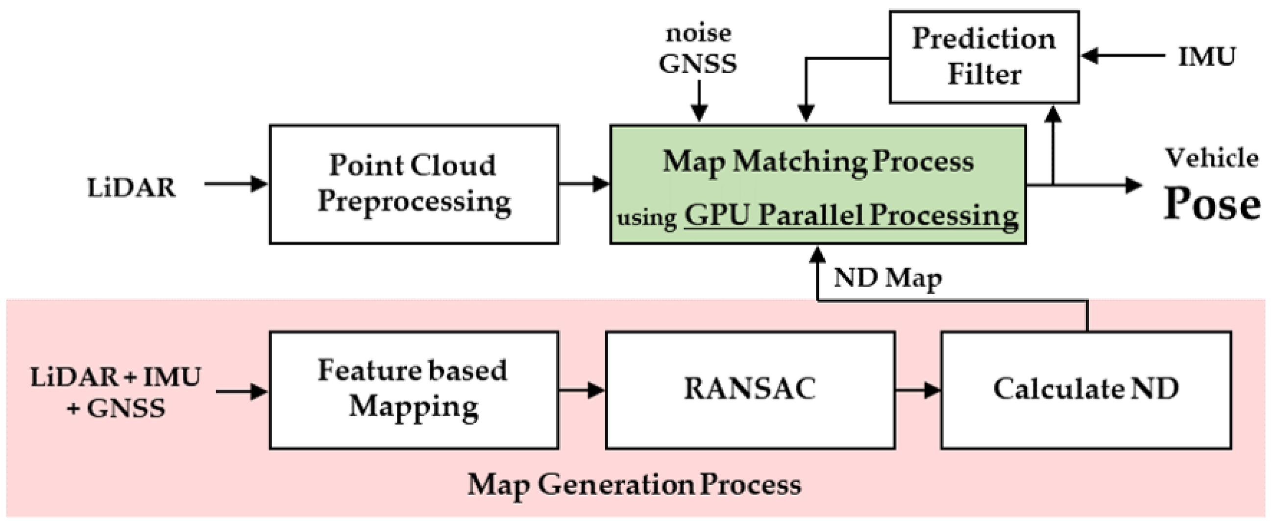
Figure 1 demonstrates a flowchart of the proposed algorithm. The red area in the figure shows the ND map generation process, which utilized measurements from three sensors (LiDAR, GNSS, and IMU) to create the map, based on universal transverse mercator (UTM) coordinates. The 3D point cloud mapping was performed based on the features of the LiDAR measurement, with the precision increased via calibration using the IMU/GNSS measurements. Subsequently, the point cloud map was converted into an ND map and used for the real-time localization process. Following the point cloud preprocessing, the pose of the ego vehicle was computed by comparing the ND map and the preprocessed point cloud. In addition, the GPU parallel processing was conducted during the map-matching process.
Figure 1 demonstrates the GPU-accelerated NDT localization algorithm flow. The resultant pose of the vehicle was entered into a prediction filter to reduce the computational time by predicting the next pose.
2.1. Map Generation
2.1.1. Global 3D Point Cloud Map
In this section, we describe the 3D point cloud map generation process. Although the 3D point cloud map generation is not the core focus of this study, it is a preliminary step that is required to create a lightweight map for localization. As the precise 3D point cloud map generation process has been extensively described in various papers, we will only briefly discuss this process.
The process was developed on the basis of the LiDAR-based SLAM algorithm, i.e., LIO-SAM, proposed by Tixiao Shan [
34]. However, unlike LOAM, scan matching is conducted using LiDAR features comprising planes and edges [
35,
36] and IMU tracking. The accumulated errors caused by odometry tracking were eliminated by loop closure, and factor graph searching efficiency was improved using GNSS data. In this study, the 3D point cloud map generation algorithm was produced by modifying the LIO-SAM algorithm according to the research environment.
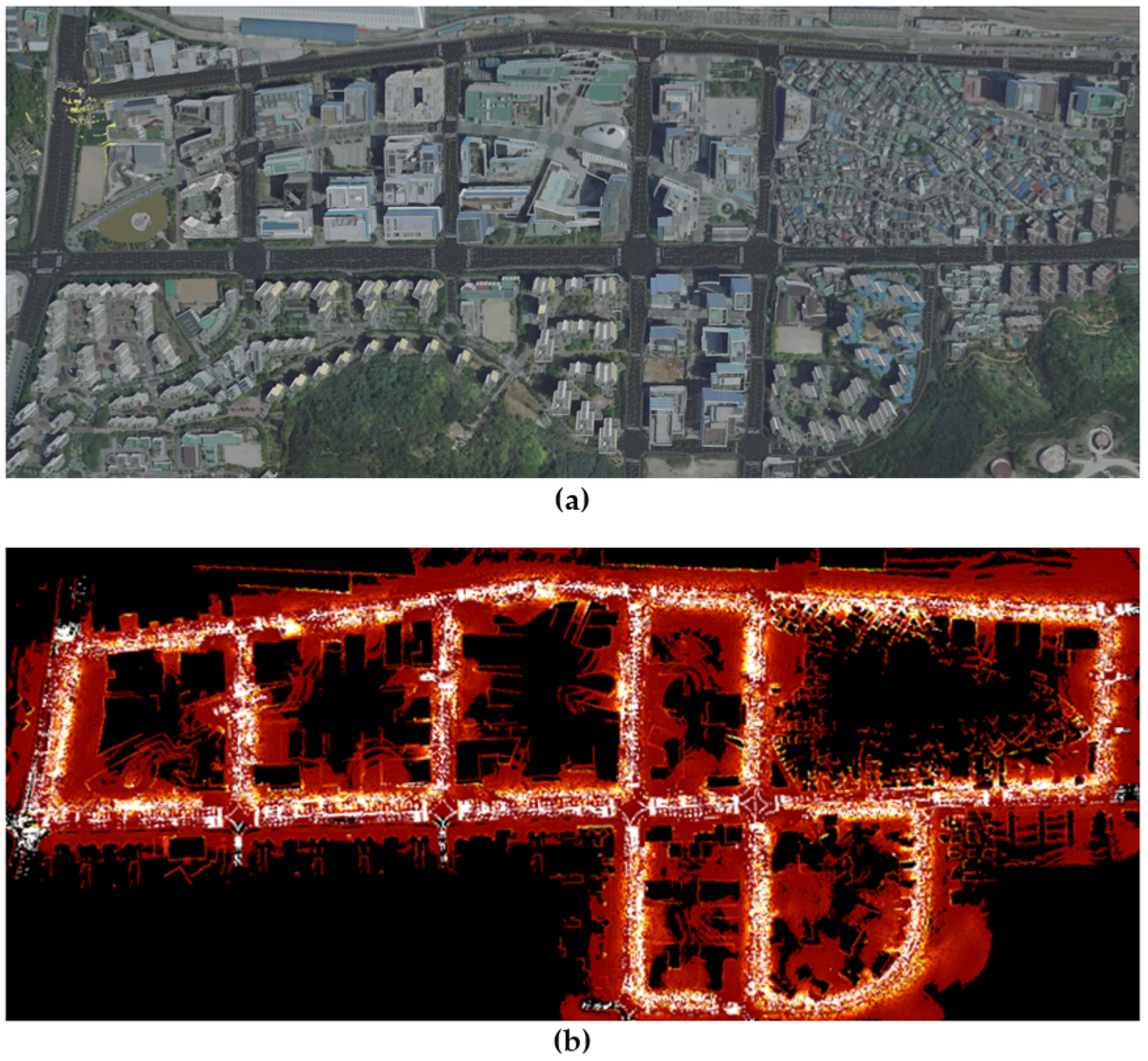
Figure 2 demonstrates the 3D point cloud map of the urban area implemented in the simulation.
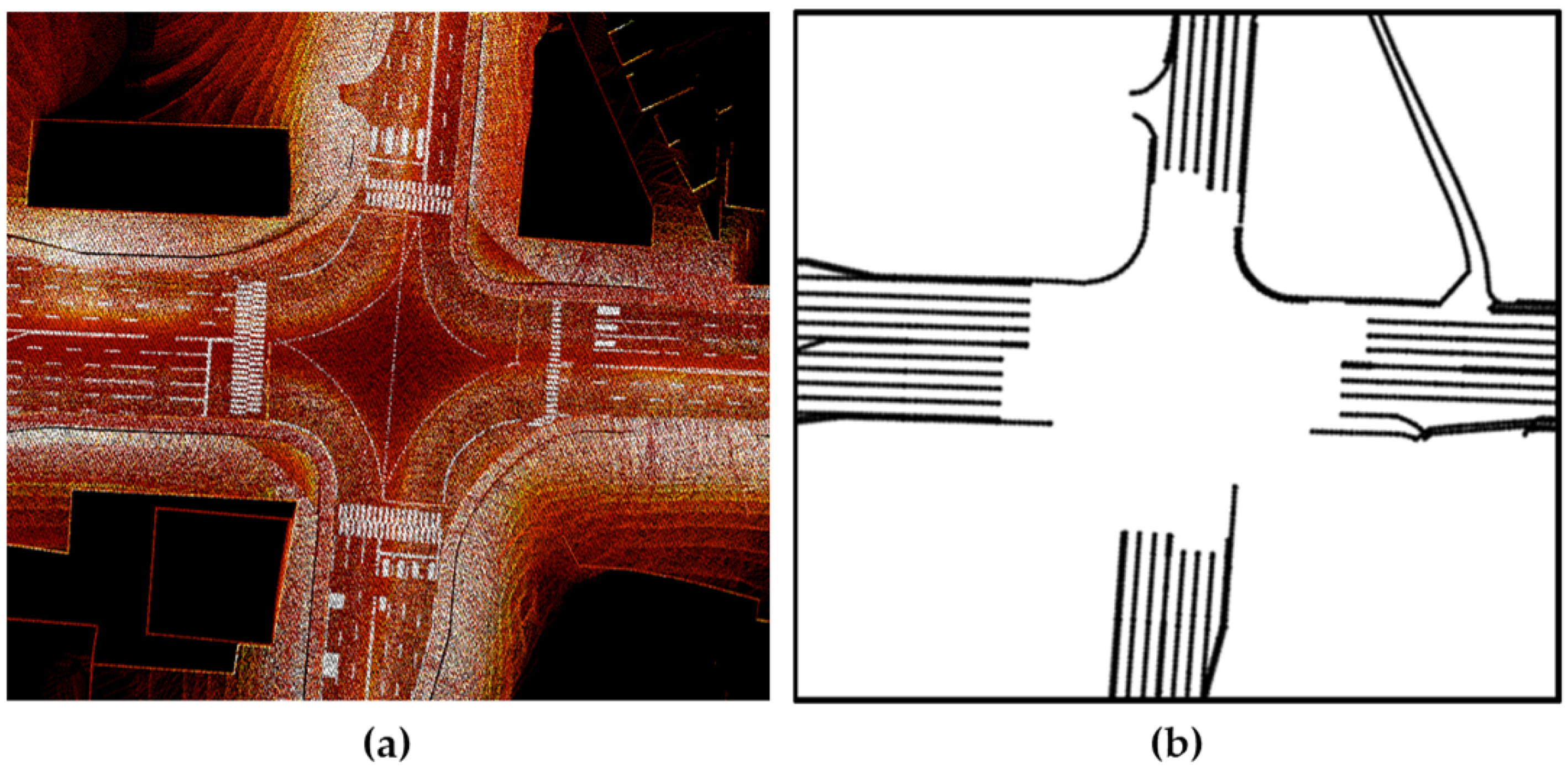
To verify the 3D point cloud map generation, lane information from a high-definition road map provided by the National Geographic Information Institute, which had a maximum error of 0.25 m, was utilized [
37]. The LiDAR sensor returned 3D coordinates (x, y, z) and reflection (intensity) data; lane information was extracted from the intensity measurements. The coordinate system of the point cloud map was converted into UTM coordinates to allow for a comparison between the common lane information in the two maps.
Figure 3 demonstrates the comparison of the intensity measurements of the point cloud map and the lane information from the high-definition road map.
2.1.2. Vector-Based Normal Distribution Transform
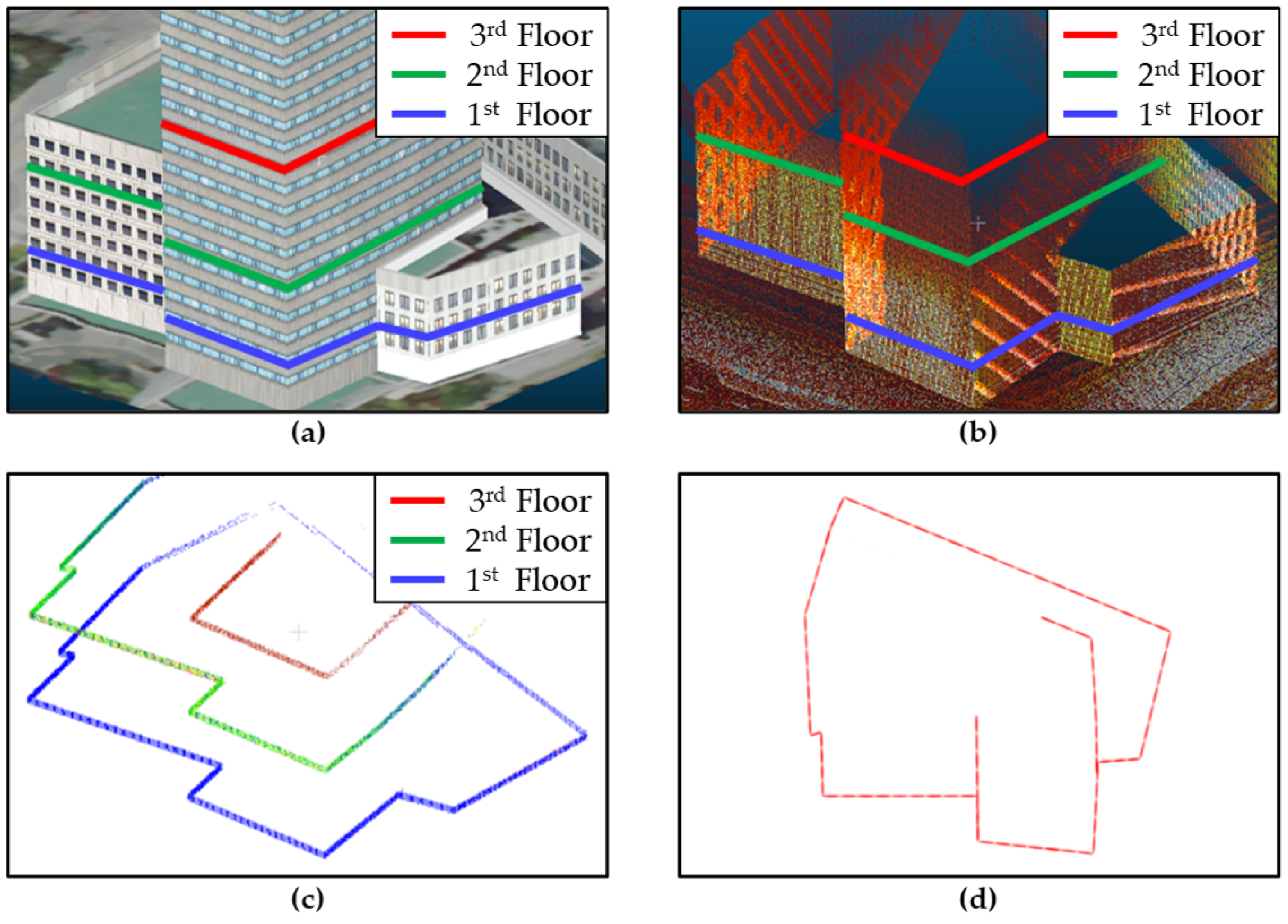
The generated 3D point cloud map extensively described the 3D information of the urban area. Generally, an autonomous driving algorithm requires a three-degree-of-freedom vehicle pose comprising x, y, and yaw, which can be obtained using a 2D map. Therefore, in this study, a 2D ND map was created from the 3D point cloud map. The location and shapes of buildings in an urban area are constant, and the location of autonomous vehicles can be uniquely identified by utilizing the shapes of these buildings using LiDAR measurements. However, some buildings in urban areas have complex 3D shapes. Therefore, multiple layers should be included in the map to represent the 3D shape of buildings, with each layer representing the shape of the cross-sections projected in the 2D plane, thereby enabling multiple layers to capture the 3D shape of a building in a 2D map.
Figure 4 shows the vector-based NDT of three representative layers of a set of urban buildings.
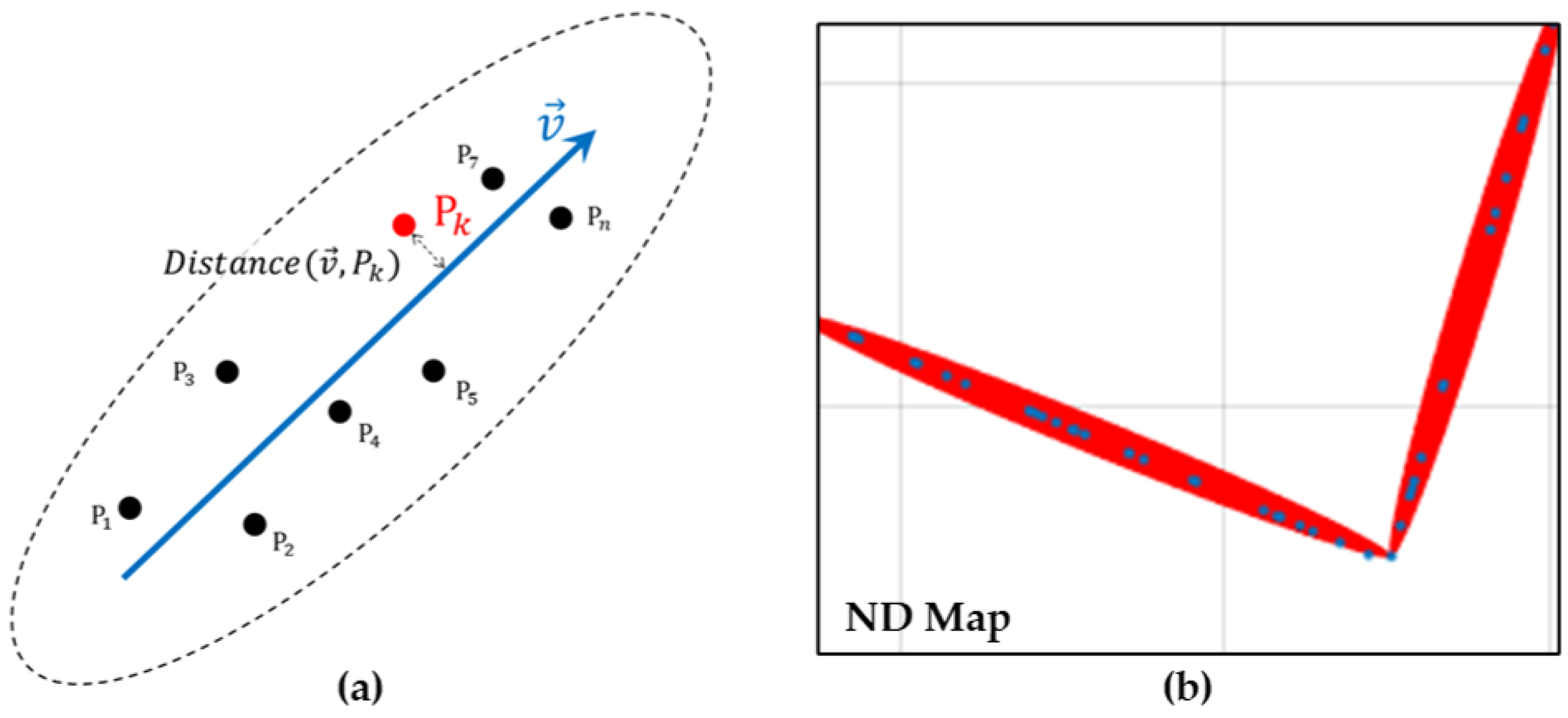
After creating the 2D point cloud map, the vectors corresponding to the walls of the buildings were extracted using the random sampling consensus (RANSAC) process. During the RANSAC process, the average vertical distance between each vector and the proximate points of the point cloud were represented using an uncertainty parameter (
), which can be calculated as follows:
where
is a vector obtained using the RANSAC process and
represents summed over positions of the point cloud near the vector. If the vector component was not properly extracted with RANSAC because of noise in the point cloud, the vector was directly designated. The vector and uncertainty information were used to calculate the covariance matrix, which represents the point cloud through NDT, using Equation (
2) as follows:
where
U is a matrix consisting of eigenvectors defined by
and its perpendicular vector,
, as follows:
where
is a matrix comprising two eigenvalues, i.e.,
and
. Eigenvalue
was set as half the length of
, and
was set as
.
Figure 5 demonstrates elements of the ND map used in Equations (1)–(4). The blue arrow in
Figure 5a represents the vector that was extracted using RANSAC, and the black points on both sides of the arrow represent the point cloud near the vector.
Figure 5b shows an approximation of the point cloud, as measured from the building wall by the ND map. The covariance matrix, i.e.,
, and the center point of
,
were stored together in the vector-based ND map file. The 3D point cloud map with an original size of 2 GB was reduced to an ND map with a size of 2 MB using the vector-based NDT process.
2.2. Map Matching Using GPU Parallel Processing
This study developed a real-time localization algorithm by comparing an ND map with LiDAR measurements. To do so, the LiDAR measurements required several preprocessing steps. First, the points in the cloud up to a height of 4 m from the road’s surface were removed to eliminate unnecessary measurements. This preprocessing method rapidly removed measurements originating from the ground and dynamic objects. Subsequently, a 3D point cloud containing only the building information was projected onto a 2D x–y plane. In addition, the real-time LiDAR measurements were not downsampled, thus enhancing the accuracy of the localization result.
The preprocessed 2D point cloud was transferred to the UTM coordinate system using the vehicle pose (position and heading angle). The 2D homogeneous matrix that was used for the transformation of the coordinate is shown in Equation (
5).
The transformed point cloud, i.e.,
, was used to determine the nearest vector,
, in the ND map. Subsequently, the score was calculated using Equation (
6), where
represents the center point of
and
represents the covariance matrix of
.
After the score was calculated, the Cost for each
was calculated by summing over the scores, as shown in Equation (
7). The negative sign was applied to modify the sum of scores as a minimization problem.
Thereafter, Newton’s method for optimization was applied to the Cost to repeatedly correct the pose toward the minimum value of the Cost. The calculation of the change in the pose, i.e.,
, used a Hessian/gradient matrix, as expressed in Equation (
8) below.
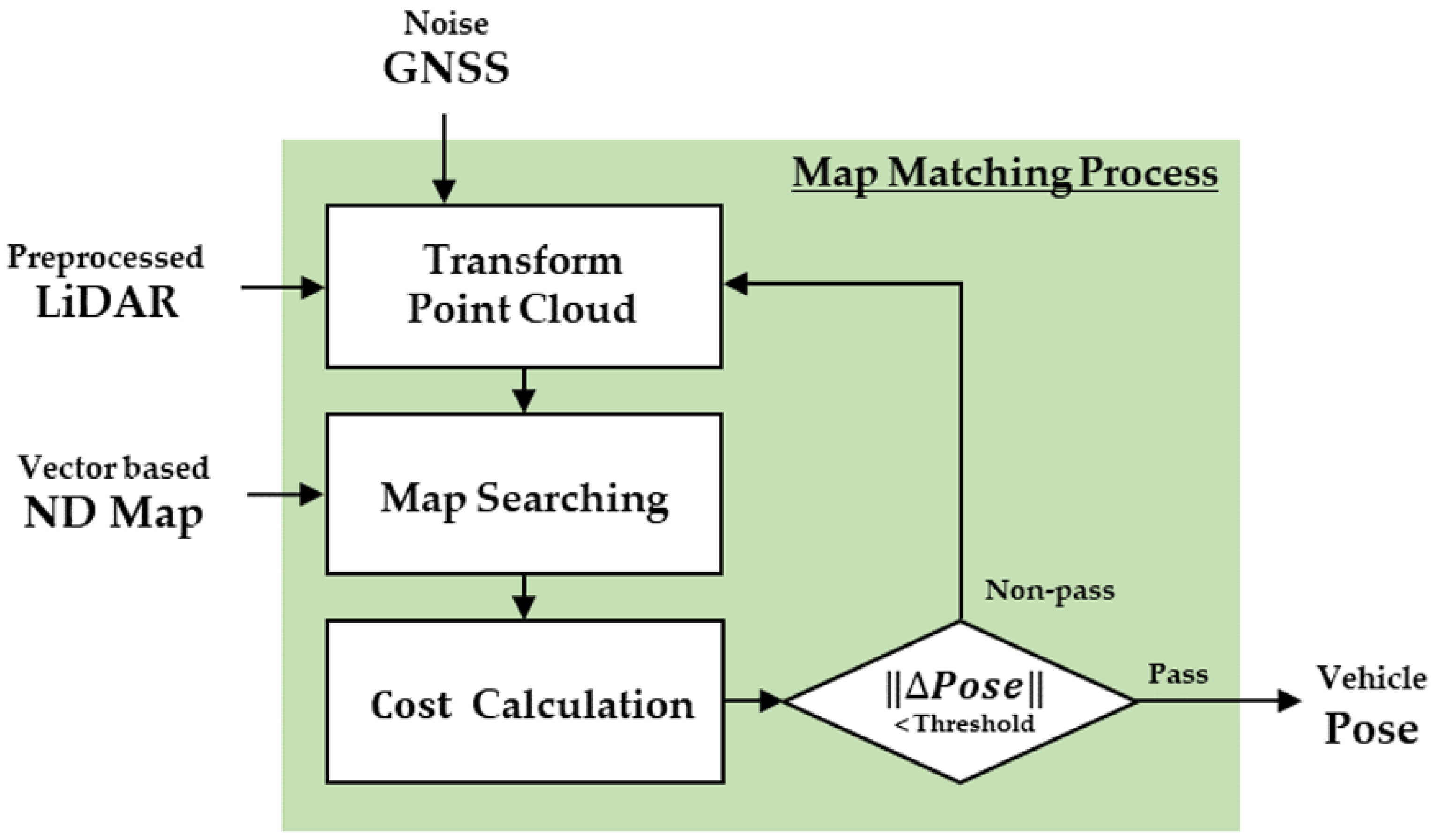
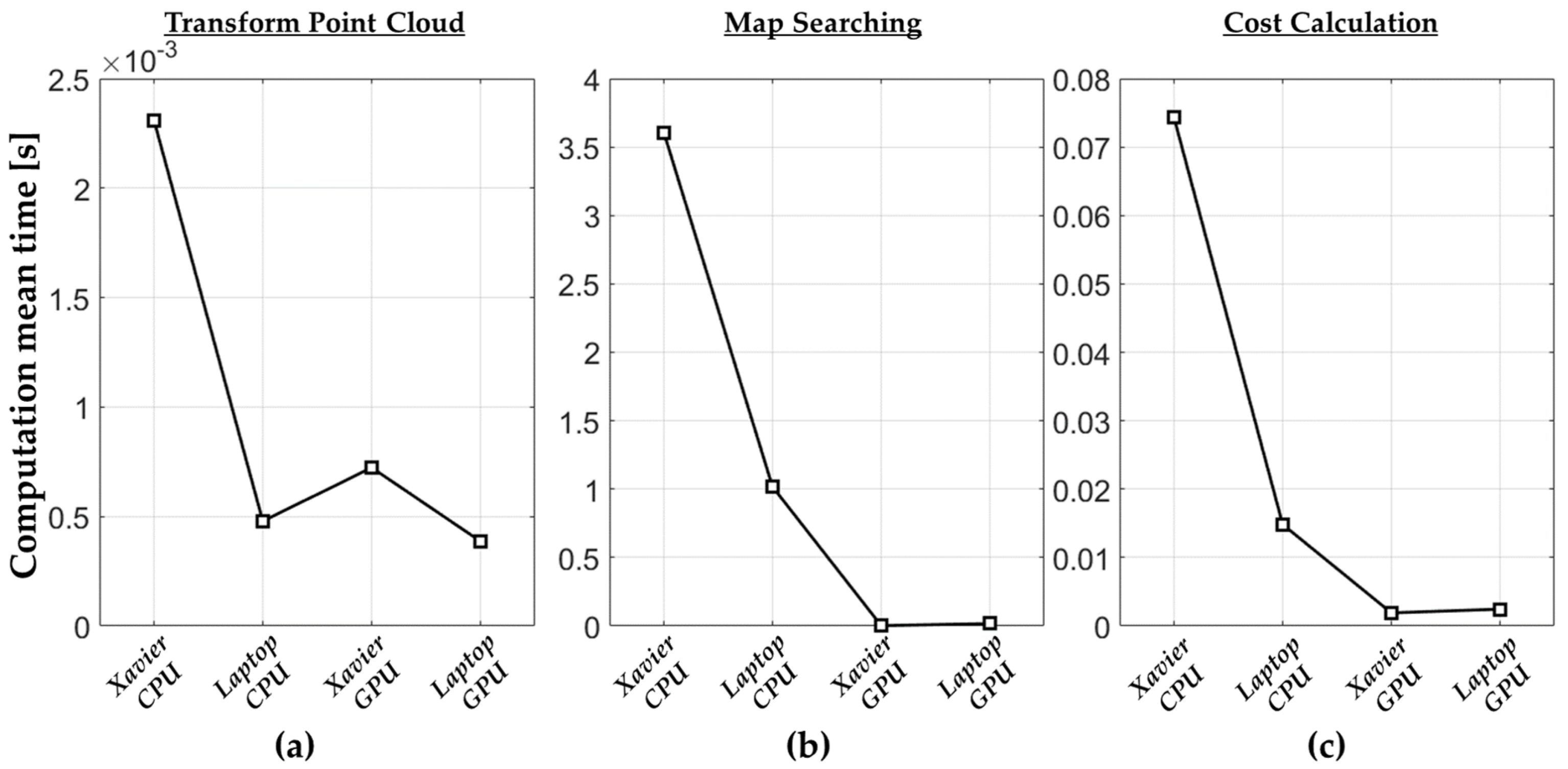
Figure 6 demonstrates a flowchart of the map-matching process between the ND map and the point cloud. The map-matching process was performed for all points in the cloud and was repeated until an appropriate pose was obtained. The computation time of the overall map-matching process increased with an increase in the number of point clouds. To reduce the overall computation time, this study used GPU parallel processing for the map-matching process.
For GPU parallel processing, a large amount of the point cloud was moved from the central processing unit (CPU; Host) memory to the GPU (Device) memory, after which the operations on each point were performed parallelly in the GPU thread. This ensured that an operation that needed to be repeated N times on the CPU could be executed at once on the N threads of the GPU. As the size of data to be computed increased, the efficiency of the GPU parallel processing increased compared with that of the CPU serial processing [
38]. However, not all operations were suitable for parallel processing. Therefore, to take advantage of parallel processing, the algorithm should comprise numerous simple iterative operations rather than a small number of complex branching operations. The localization algorithm proposed in this study was suitable for GPU parallel processing as the same operations, Equations (
5)–(
8), were repeated for all points
in the point cloud. However, when a large number of individually calculated values from all point clouds had to be added to obtain a single value, bottlenecks were observed in the map-matching process.
2.2.1. GPU Parallel Reduction
In this study, the bottlenecks of the map-matching process were resolved using parallel reduction [
39].
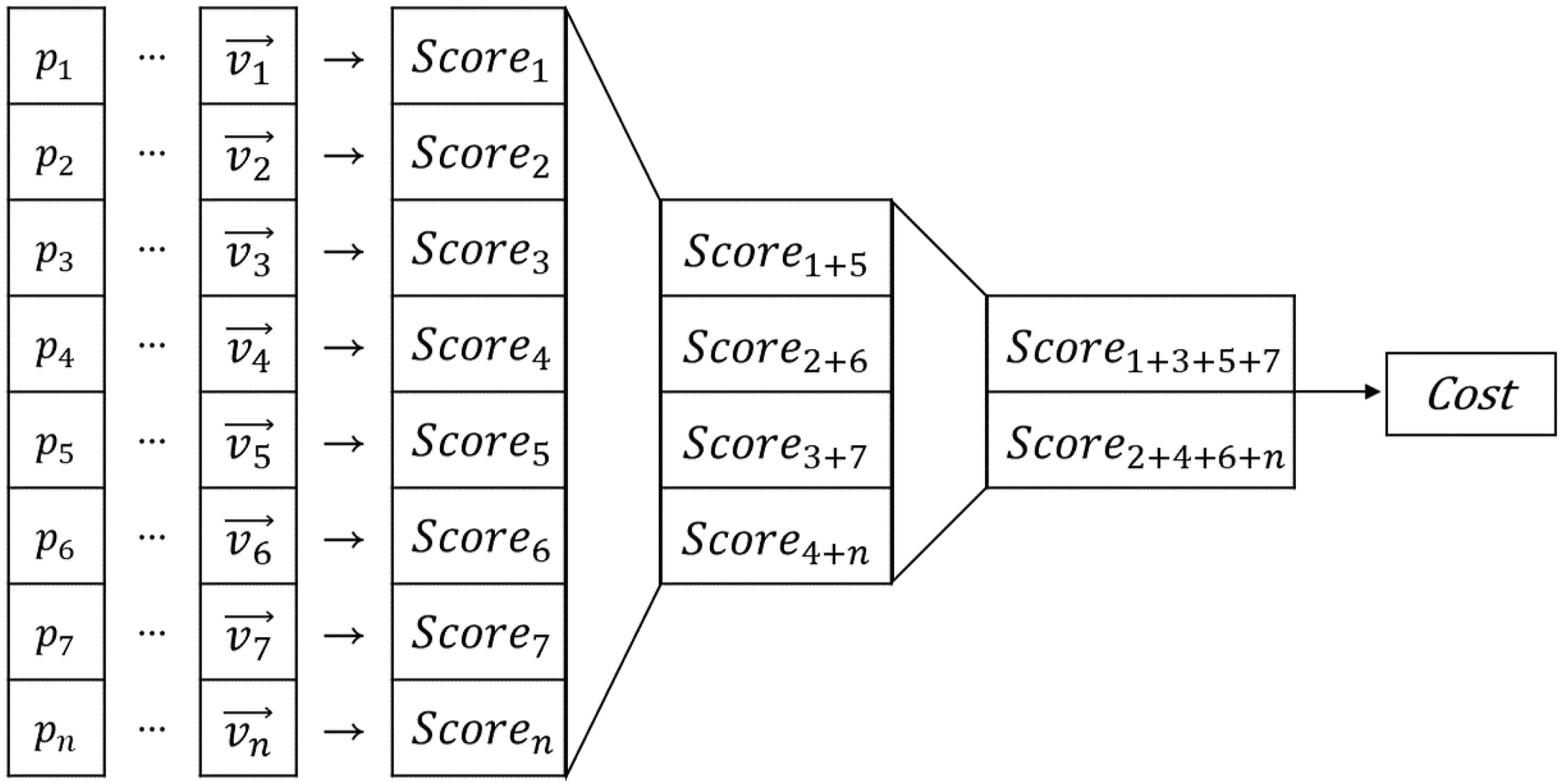
Figure 7 shows the computational flow of a cost calculation in which the parallel reduction was applied. To utilize CPU serial processing for the cost calculation, the addition of the score value to the cost value was repeated consecutively. In contrast, the parallel reduction performed a tree-type addition to obtain the final overall sum by repeating the individual additions of two pieces of data (
Figure 7). The parallel reduction process reduced the number of operations conducted from N to
. Algorithm 1 represents the pseudocode of the parallel cost calculation. Different GPU threads were used to simultaneously compute the score between each point and the nearest vector. Next, threads that were separated by a specific index were added together. These computations were conducted for only half of the total threads, and the number of threads subjected to these computations was continuously reduced by half to ensure that the operation was conducted only on the first thread. Following the parallel reduction, the sum of all the scores was computed.
When the parallel reduction was performed, the score data were repeatedly loaded. However, storage of the score data in the global memory resulted in unnecessary repetition of the data transfer delay between the thread and the global memory during operation [
40]. Therefore, the score data were transferred from the global memory to the shared memory in advance to minimize the delay caused by data loading.
| Algorithm 1: Parallel Cost Calculation |
![Sensors 22 01913 i001]() |
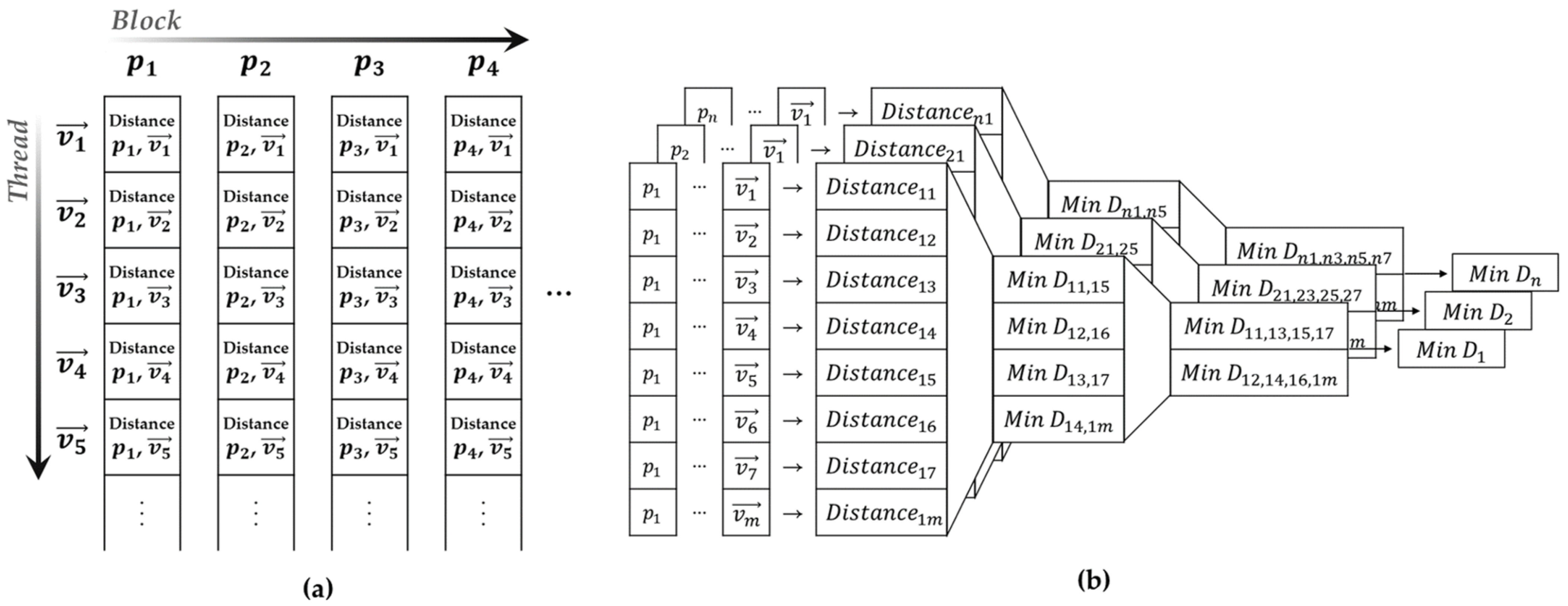
Before conducting the cost calculation, map searching was conducted to determine the closest vector to each point. A parallel reduction was applied to the comparison operation during this process. In contrast to the cost calculation, a parallel reduction was conducted separately for each point. As shown in
Figure 8a, different points are loaded in each GPU block, and the distances from these points to all vectors are calculated. Subsequently, parallel reduction was individually conducted for each block, as shown in
Figure 8b. Thereafter, the nearest vector for each block was calculated using the map-searching results. Algorithm 2 represents the pseudocode of the parallel map searching.
| Algorithm 2: Parallel Map Searching |
![Sensors 22 01913 i002]() |
3. Experiments
In this study, the proposed algorithm was developed on the basis of a C/C++ robot operating system in Ubuntu 18.04 (Canonical Ltd., London, UK). The computation was accelerated using the GPU parallel processing abilities of the CUDA platform (NVIDIA Corporation, Santa Clara, CA, USA).
Table 1 shows the detailed specifications of the computing system used for verification.
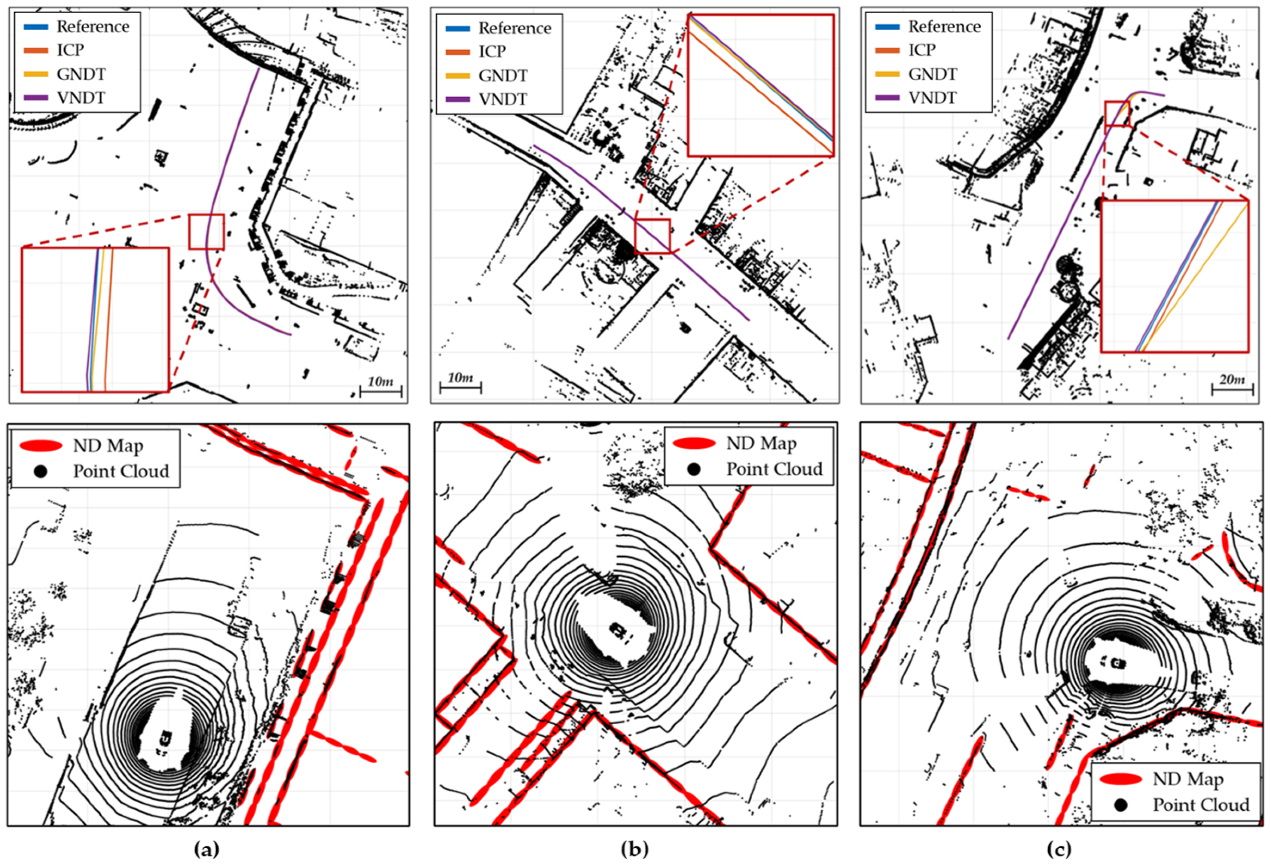
The proposed vector-based normal distribution, i.e., VNDT, was compared with other localization methods—specifically, iterative closest point, i.e., ICP, and grid-based normal distribution transform, i.e., GNDT, [
32,
41]. In this study, we used corresponding algorithms that were implemented on the Point Cloud Library [
42]. The tuning parameters common to all algorithms were the maximum number of iterations and the iteration tolerance. The maximum number of iterations was set to 50, and the iteration tolerances were set to 0.1 cm and 0.01
. Detailed descriptions of the tuning parameters for these algorithms are available in [
43,
44]. In addition, the grid size and vector length are important tuning parameters for NDT algorithms. In this study, these parameters were set to 2 m.
3.1. Open Datasets
To verify the performance of the algorithm with real sensor data, including noise, the nuScenes dataset was used [
45]. The nuScenes dataset is a public dataset for autonomous driving developed by an autonomous vehicle company, Motional. Scenes containing complex driving environments in Boston and Singapore were selected from the dataset. The reasons for choosing each scene are as follows.
scene-0061: The scene data were recorded from Singapore’s One North. The driving route at an intersection was under construction. Using the scene data, the accuracy of localization in a congested situation (e.g., passersby standing before traffic signals, construction machine on the road) was verified.
scene-0103: The scene data were recorded from Boston Seaport. The driving route started at the Congress Street Bridge with no buildings nearby. Using the scene data, the initialization of localization was verified with distant building information.
scene-1094: The scene data were recorded from Singapore’s Queenstown. Since the vehicle was driven on a rainy road at night, the LiDAR measurement was unstable. Using the scene data, the accuracy of localization was verified using the unstable LiDAR measurement.
Each scene included ego pose data that had been precisely calibrated using a point cloud map provided by Motional. In this study, the ND map was produced by stacking point cloud data according to the corresponding ego pose. The driving time for acquiring each scene’s data was 20 s, and the data from each sensor (LiDAR, GPS, IMU, etc.) and the calibrated ego pose were stored at a constant rate of 2 Hz. The driving distances for each scene were 91 m (scene-0061), 118 m (scene-0103), and 126 m (scene-1094).
Figure 9 demonstrates the driving route of each scene.
3.2. Simulation
The CarMaker simulation program (IPG Automotive GmbH) was used to verify the computational efficiency with long-term driving. To conduct the localization at the same coordinates as the real urban area, the CarMaker simulation was developed according to the high-definition road map information provided by the National Geographic Information Institute of Korea. It was also possible to implement the simulated buildings with a shape and density very similar to reality by referring to photos of urban areas.
Figure 10 shows a comparison of the real and simulated urban areas.
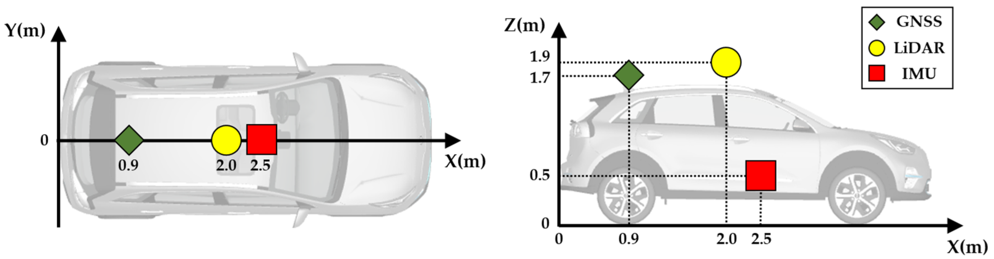
Simulated driving was conducted using a simulation vehicle equipped with LiDAR, GNSS, and IMU sensors in CarMaker. To enhance the realism of the simulation, the vehicle was developed according to the specifications of the KIA Niro.
Table 2 lists the detailed specifications.
Table 3 lists the detailed specifications of the simulation LiDAR sensor, which was implemented by referring to Ouster’s OS1-64 model.
Considering that there was no error in the GNSS within the simulation, a radial uniform distribution error of 2 m was introduced. The noise in the GNSS reading was used as the initial pose in the localization algorithm, and the original GNSS was used only to represent the ground truth for evaluating the performance of the algorithm.
Figure 11 shows the position of the sensors attached to the simulation vehicle. The LiDAR sensor was placed at the center of the front seat of the vehicle and was installed 15 cm above the vehicle roof to reduce the shadow area. The GNSS sensor was attached to the center of the roof above the rear wheel axle, and the IMU sensor, which was used to track the vehicle odometry, was placed at the vehicle’s center of gravity.
The length of the verification route was 4300 m, and the total driving time was 7 min. During the simulation, the vehicle moved at a speed of 60 km/h using the CarMaker auto-driving system. Since localization was conducted on all LiDAR inputs (10 Hz), the root-mean-square error (RMSE) was calculated with more than 4000 resultant data points.
Figure 12 shows the verification route in CarMaker.
5. Conclusions
In this study, we introduced a GPU-accelerated vector-based NDT localization algorithm that could guarantee precision and real-time performance for 10–20 Hz high-resolution LiDAR, even in GNSS-denied urban areas. Therefore, a vector-based ND map suitable for the parallel processing algorithm was used for the reference map. Parallel processing was applied to the map-matching process to maintain a stable and fast computational speed, regardless of the size of the LiDAR measurement data. In particular, the parallel reduction was used for map searching and the cost calculation function of the map-matching process. The performance of the proposed algorithm was evaluated with the nuScenes open dataset and urban environment in a CarMaker simulation. The performance of the proposed algorithm satisfied the accuracy required by ISO 17572. In addition, the fast computational speed of the algorithm enabled a localization update rate of 10 Hz. Therefore, the proposed algorithm exhibited enhanced computational speed and highly reliable performance. In a future study, we plan to study localization in the actual urban area that was referenced in the simulation. We will propose a robust localization algorithm for the real environment and analyze the GPU efficiency in detail.


