
A New LoRa-like Transceiver Suited for LEO Satellite Communications †


Abstract
:1. Introduction
- 1.
- The presence of carrier frequency offset (CFO) causes a shift of all the Fourier transform peaks of a sequence of symbols to the right or the left of the desired frequency peak locations.
- 2.
- A sampling time offset (STO) causes the emergence of two main shifted peaks in the spectrum, which lead to inter-symbol interference (ISI).
- Modify the CSS modulation in order to enhance its robustness to time and frequency synchronization errors, especially when the latter are time varying. Subsequently, our approach would allow to deal with Doppler shifts with much faster variations in time than the existent LoRa-like receivers.
- Release the constraint of a maximum allowed CFO of caused by the classical synchronization algorithms in LoRa [14,19,20,26,27]. To address this, the time synchronization is implemented regardless for the CFO. Currently, the frequency mismatch of local oscillators (LOs) between the transmitter and the receiver in LoRa-based communications do not reach this value maximum allowed CFO. However, this mismatch of LOs, combined with significant Doppler shifts, in the context of LEO communications, could lead to a CFO that exceeds the quarter of the bandwidth. Hence, with our approach, we can propose reducing the bandwidth of the chirped signals, without worrying about the occurrence of a CFO that exceeds the latter constraint, which would provide a gain in sensitivity (the actual choices of bandwidth for LoRa-like signal are based on the local oscillator precision to satisfy the constraint) and increase the capacity of LoRa-based networks.
2. Synchronization Issues in LoRa
2.1. LoRa Physical Layer Principle
2.2. Analysis of Imperfect Synchronization on Symbol Estimation
- Time varying Doppler frequency shift, , with the Doppler rate (DR) and is the Doppler shift;
- Uniformly distributed STO .
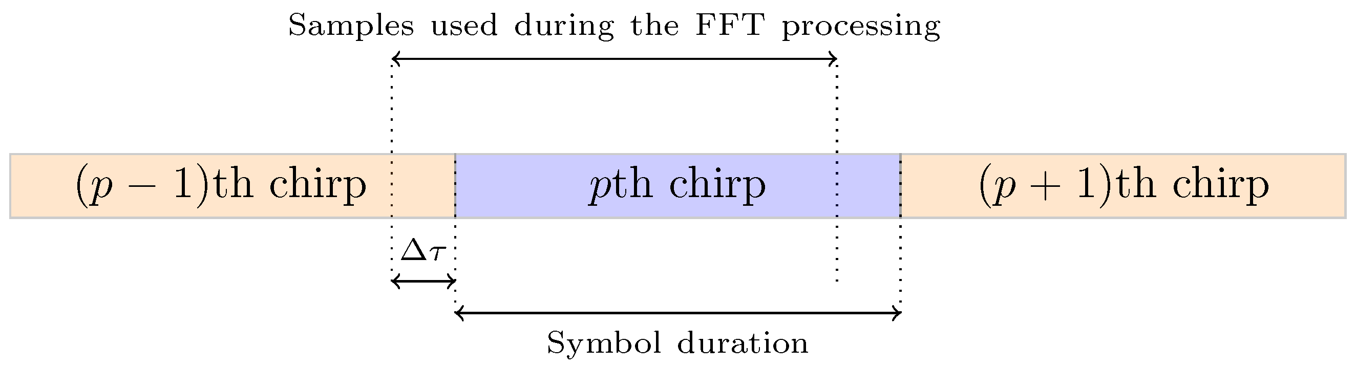
- A contribution of the transmitted chirp during the time interval ;
- A contribution of the transmitted chirp during the time interval ;
2.2.1. Impact of the CFO and the STO on Symbol Estimation
- is an integer offset that shifts all the symbols;
- is the fractional part of the CFO that shifts the spectrum line between two frequency bins, effectively making a kernel appears in the frequency domain.
2.2.2. Impact of the Doppler Rate on Symbol Estimation
2.3. Insights on Strategies Used to Synchronize LoRa Signals
2.3.1. Structure of the Synchronization Signal
2.3.2. Synchronization Process in LoRa
3. Proposed Transceiver
3.1. Differential Chirp Spread Spectrum
3.1.1. Principle
3.1.2. Additional Processing at the Receiver
- Quadratic interpolation;
- Secant method;
- Newton’s method;
- Bisection method.
- 1.
- Consider a number of points that are of a power of two. More precisely, and are taken. The starting analysis interval is
- 2.
- Estimate at the extremities and , and also at the two points “in the middle” of the analysis interval, i.e., and . If the maximum of calculated in these four points is reached for for one of the two extremities of “half” left , this interval becomes the new analysis interval, otherwise the new analysis interval will be the “half” right .
- 3.
- Loop on step 2 by processing the new analysis interval and continue until step 4 criteria is reached.
- 4.
- After p iterations, the extremities of the analysis interval are two points at a distance of . The highest value of computed from these points is decided to be the sought solution.
3.2. Proposed Synchronization Signal Based on the Use of DCSS
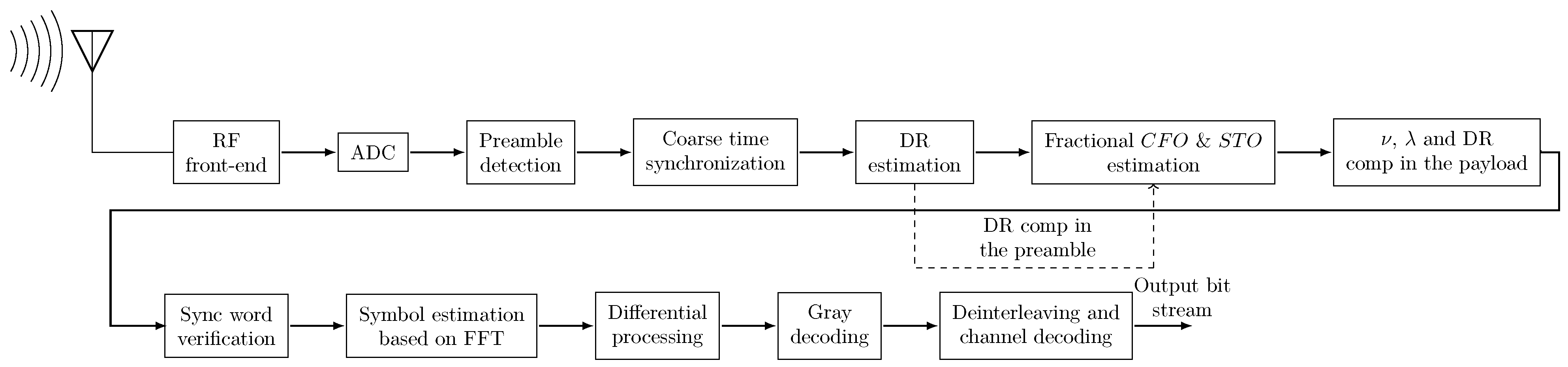
3.3. Proposed Synchronization Algorithm
- 1.
- Preamble detection;
- 2.
- Coarse time synchronization;
- 3.
- Doppler rate estimation;
- 4.
- Fractional CFO estimation;
- 5.
- Fractional STO estimation;
- 6.
- DR, fractional CFO, and fractional STO compensations.
3.3.1. Step 1—Preamble Detection
3.3.2. Step 2—Coarse Time Synchronization
| Algorithm 1: Proposed estimation of . |
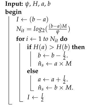 |
3.3.3. Step 3—Doppler Rate Estimation
- (i)
- Estimate the of the FFT module in each symbol interval of the preamble. If we note , the of the FFT module in the T-long sequence, we have:with and , . It should be noted here that the interpolation method, as presented in Section 3.1.2, is used to increase the accuracy of the estimate , while in [22], a classical function, is performed.
- (ii)
- The FFT is used in pairs to compute different DR estimates noted . These estimations are obtained using the couple , with and . Thus, by considering (17), we have:
- (iii)
- An estimation of the DR is obtained by averaging , as follows:
3.3.4. Step 4—Fractional CFO Estimation
3.3.5. Step 5—Fractional STO Estimation
3.3.6. Step 6—DR, Fractional CFO, and Fractional STO Compensation
4. Results and Discussion
- A number of preamble up-chirps ;
- A reference bandwidth kHz, which is the most commonly used bandwidth in LoRa-based networks;
- An oversampling factor , which gives a typical sampling frequency in LoRa receivers MHz, when the bandwidth of the signal is equal to ;
- (respectively, ) uniformly distributed in (respectively, ).
4.1. Channel Coding and Interleaving in LoRa
4.1.1. Interleaving
4.1.2. Forward Error Correction
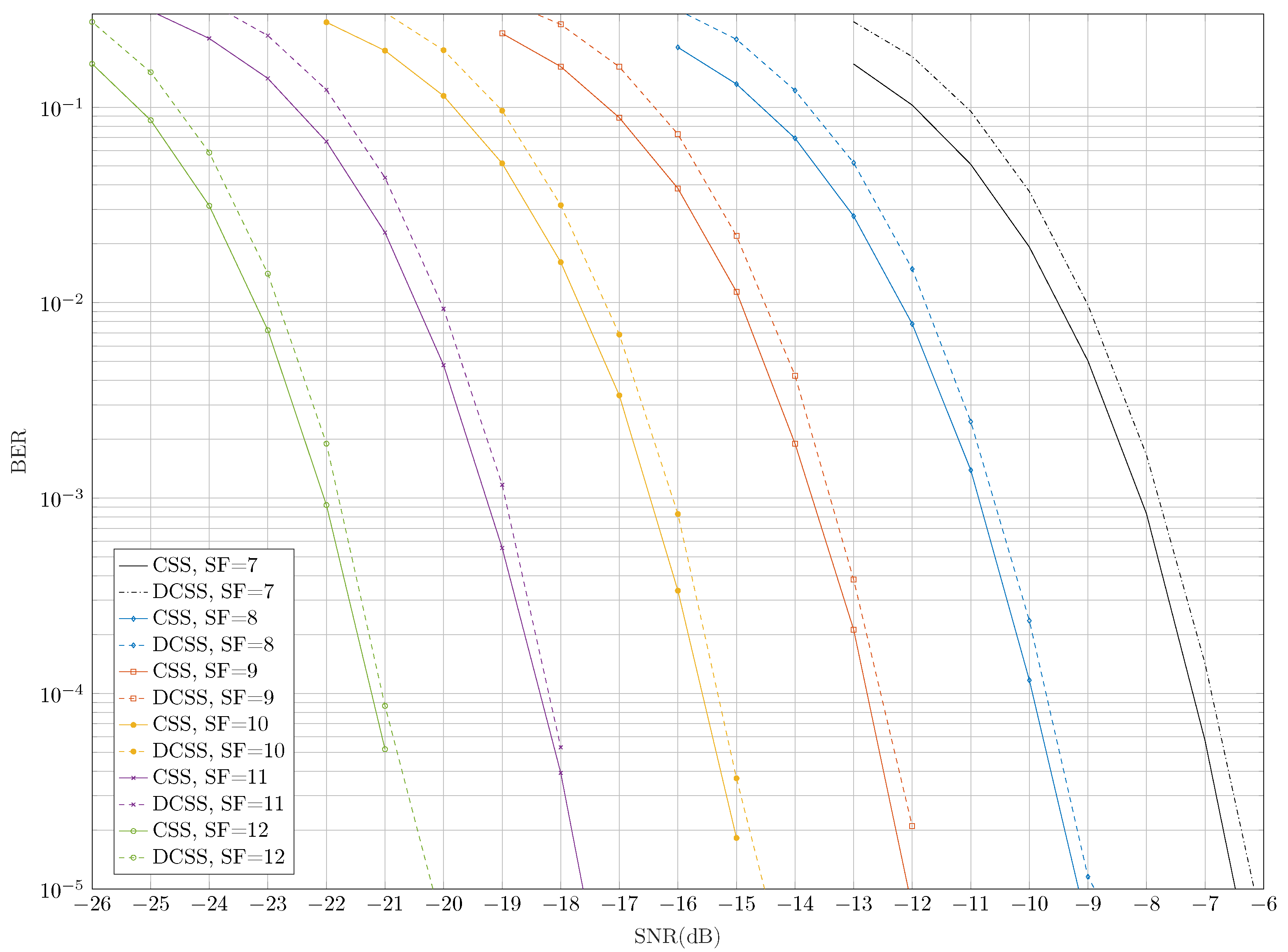
4.2. DCSS Performance Evaluation and Comparison with CSS
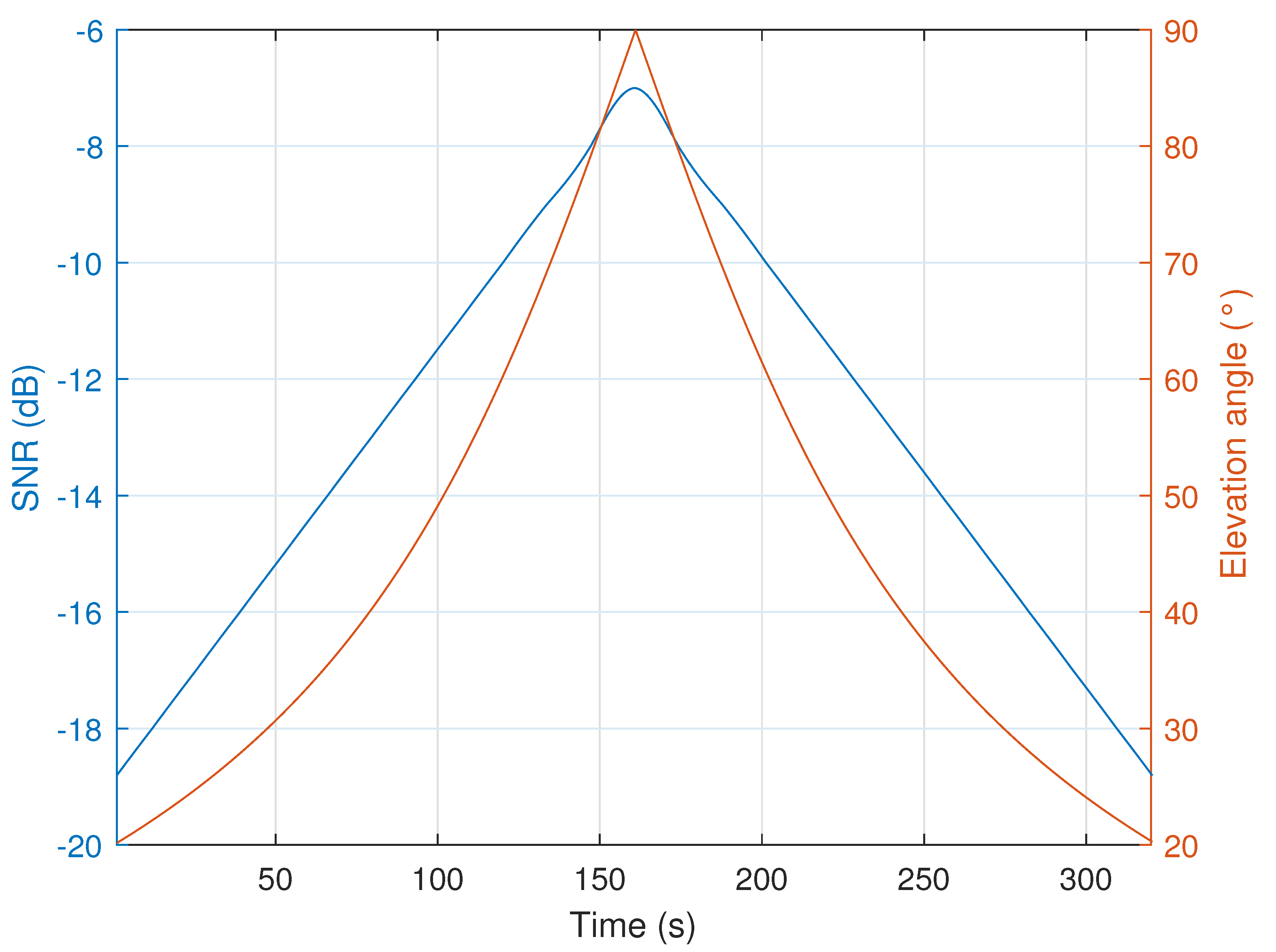
4.3. Evaluating the Proposed Receiver with LEO Satellite Communication
4.3.1. Synchronization Algorithm Numerical Results
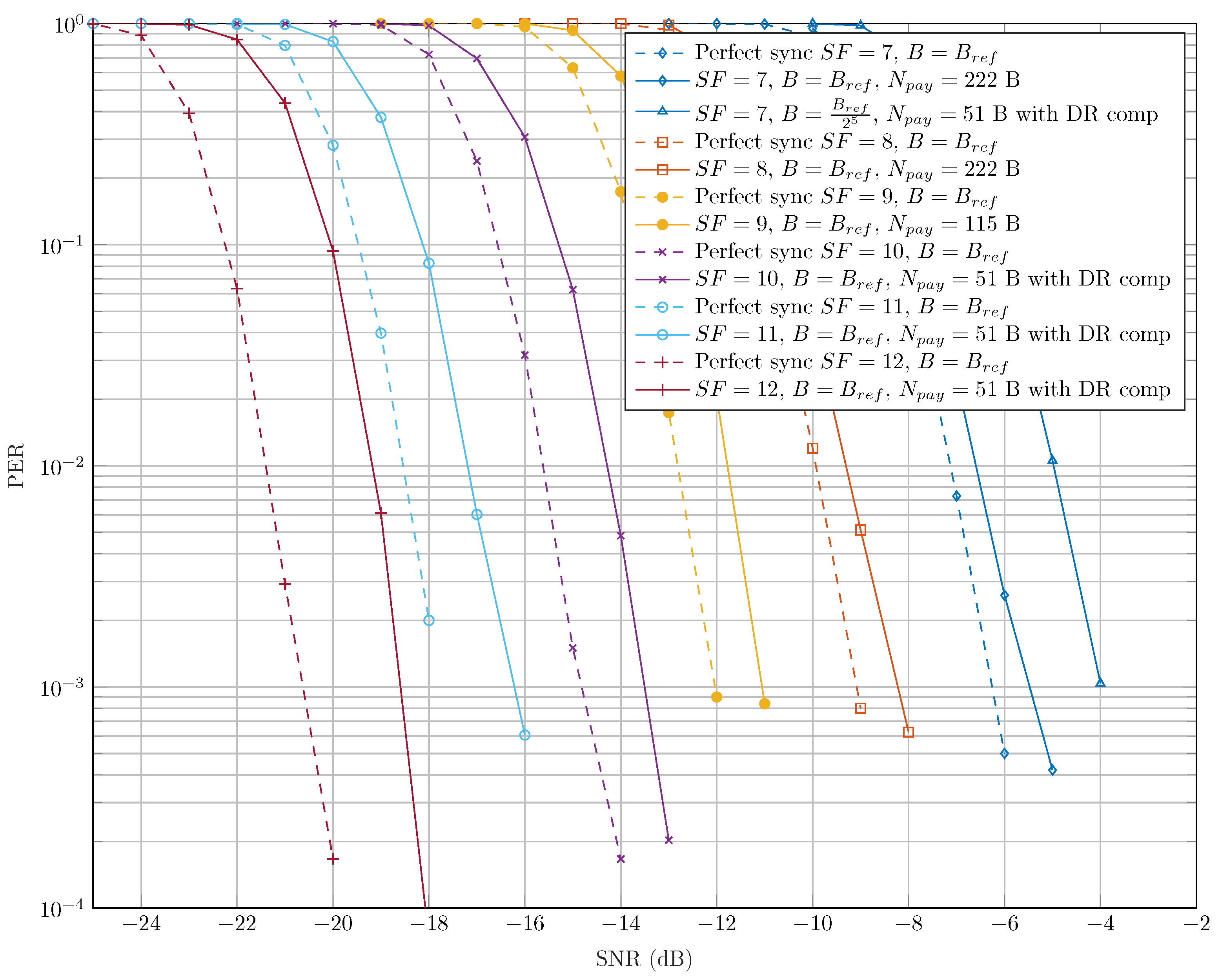
4.3.2. Decoding Performance of the Proposed Receiver
5. Conclusions
Author Contributions
Funding
Data Availability Statement
Conflicts of Interest
References
- Cisco. Cisco Visual Networking Index: Cisco Annual Internet Report (2018–2023); White Paper; Cisco: San Jose, CA, USA, 2018. [Google Scholar]
- Raza, U.; Kulkarni, P.; Sooriyabandara, M. Low Power Wide Area Networks: An Overview. IEEE Commun. Surv. Tutor. 2017, 19, 855–873. [Google Scholar] [CrossRef] [Green Version]
- Sigfox. Sigfox—The Global Communications Service Provider for the Internet of Things (IoT). 2018. Available online: https://www.sigfox.com/en (accessed on 2 June 2021).
- Semtech. LoRa Modem Design Guide: Sx1272/3/6/7/8. 2013. Available online: https://www.openhacks.com/uploadsproductos/loradesignguide_std.pdf (accessed on 2 June 2021).
- Eutelsat. Satellite IOT: A Compliment to Cellular. 2020. Available online: https://www.eutelsat.com/fr/home/news--resources/blog/satellite-for-iot-a-complement-to-cellular.html (accessed on 2 June 2021).
- Barbau, R.; Deslandes, V.; Jakllari, G.; Tronc, J.; Chouteau, J.F.; Beylot, A.L. NB-IoT over GEO Satellite: Performance Analysis. In Proceedings of the 2020 10th Advanced Satellite Multimedia Systems Conference and the 16th Signal Processing for Space Communications Workshop (ASMS/SPSC), Graz, Austria, 20–21 October 2020; pp. 1–8. [Google Scholar] [CrossRef]
- Sigfox. Admiral LEO World-Wide Coverage Service of Satellite and Terrestrial IoT. 2019. Available online: https://www.sigfox.com/sites/default/files/2019-11/Flyer%20_%20sigfox%20LEO%20.pdf (accessed on 2 June 2021).
- Temim, M.A.B.; Ferré, G.; Laporte-Fauret, B.; Dallet, D.; Minger, B.; Fuché, L. An Enhanced Receiver to Decode Superposed LoRa-like Signals. IEEE Internet Things J. 2020, 7, 7419–7431. [Google Scholar] [CrossRef]
- Ben Temim, M.A.; Ferré, G.; Tajan, R. Analysis of the Coexistence of Ultra Narrow Band and Spread Spectrum Technologies in ISM Bands. In International Symposium on Ubiquitous Networking; Springer International Publishing: Cham, Switzerland, 2020; pp. 56–67. [Google Scholar]
- Wu, T.; Qu, D.; Zhang, G. Research on LoRa Adaptability in the LEO Satellites Internet of Things. In Proceedings of the 2019 15th International Wireless Communications Mobile Computing Conference (IWCMC), Tangier, Morocco, 24–28 June 2019; pp. 131–135. [Google Scholar] [CrossRef]
- Reichman, A. Enhanced Spread Spectrum Aloha (E-SSA), an emerging satellite return link messaging scheme. In Proceedings of the 2014 IEEE 28th Convention of Electrical Electronics Engineers in Israel (IEEEI), Eilat, Israel, 3–5 December 2014; pp. 1–4. [Google Scholar] [CrossRef]
- De Gaudenzi, R.; del Río Herrero, O.; Acar, G.; Garrido Barrabés, E. Asynchronous Contention Resolution Diversity ALOHA: Making CRDSA Truly Asynchronous. IEEE Trans. Wirel. Commun. 2014, 13, 6193–6206. [Google Scholar] [CrossRef]
- Seller, O.; Sornin, N. Low Power Long Range Transmitter. U.S. Patent 9,252,834B2, 2 February 2016. [Google Scholar]
- Seller, O.; Sornin, N. Low Complexity, Low Power and Long Range Radio Receiver. U.S. Patent 10,305,535B2, 28 May 2019. [Google Scholar]
- Elshabrawy, T.; Robert, J. Analysis of BER and Coverage Performance of LoRa Modulation under Same Spreading Factor Interference. In Proceedings of the 2018 IEEE 29th Annual International Symposium on Personal, Indoor and Mobile Radio Communications (PIMRC), Bologna, Italy, 9–12 September 2018; pp. 1–6. [Google Scholar] [CrossRef]
- Liando, J.; Gamage, A.; Tengourtius, A.; Li, M. Known and Unknown Facts of LoRa: Experiences from a Large-scale Measurement Study. ACM Trans. Sens. Netw. 2019, 15, 1–35. [Google Scholar] [CrossRef]
- Al Homssi, B.; Dakic, K.; Maselli, S.; Wolf, H.; Kandeepan, S.; Al-Hourani, A. IoT Network Design Using Open-Source LoRa Coverage Emulator. IEEE Access 2021, 9, 53636–53646. [Google Scholar] [CrossRef]
- Reynders, B.; Pollin, S. Chirp spread spectrum as a modulation technique for long range communication. In Proceedings of the 2016 Symposium on Communications and Vehicular Technologies (SCVT), Mons, Belgium, 22 November 2016; pp. 1–5. [Google Scholar] [CrossRef]
- Bernier, C.; Dehmas, F.; Deparis, N. Low Complexity LoRa Frame Synchronization for Ultra-Low Power Software-Defined Radios. IEEE Trans. Commun. 2020, 68, 3140–3152. [Google Scholar] [CrossRef] [Green Version]
- Semtech. 2019. Available online: https://www.semtech.com/ (accessed on 28 March 2019).
- Ben Temim, M.A.; Ferré, G.; Tajan, R. A Novel Approach to Enhance the Robustness of LoRa-Like PHY Layer to Synchronization Errors. In Proceedings of the IEEE Global Communications Conference (GLOBECOM 2020), Taipei, Taiwan, 7–11 December 2020. [Google Scholar]
- Colavolpe, G.; Foggi, T.; Ricciulli, M.; Zanettini, Y.; Mediano-Alameda, J. Reception of LoRa Signals from LEO Satellites. IEEE Trans. Aerosp. Electron. Syst. 2019, 55, 3587–3602. [Google Scholar] [CrossRef]
- Qian, Y.; Ma, L.; Liang, X. Symmetry Chirp Spread Spectrum Modulation Used in LEO Satellite Internet of Things. IEEE Commun. Lett. 2018, 22, 2230–2233. [Google Scholar] [CrossRef]
- Qian, Y.; Ma, L.; Liang, X. The Performance of Chirp Signal Used in LEO Satellite Internet of Things. IEEE Commun. Lett. 2019, 23, 1319–1322. [Google Scholar] [CrossRef]
- Boquet, G.; Tuset, P.; Adelantado, F.; Watteyne, T.; Vilajosana, X. LoRa-E: Overview and Performance Analysis. arXiv 2020, arXiv:2010.00491. [Google Scholar]
- Semtech. Application Note: LoRa Modulation Crystal Oscillator Guidance. 2017. Available online: https://en.sekorm.com/doc/2044721.html (accessed on 2 June 2021).
- Xhonneux, M.; Bol, D.; Louveaux, J. A Low-complexity Synchronization Scheme for LoRa End Nodes. arXiv 2019, arXiv:1912.11344. [Google Scholar]
- Tapparel, J.; Afisiadis, O.; Mayoraz, P.; Balatsoukas-Stimming, A.; Burg, A. An Open-Source LoRa Physical Layer Prototype on GNU Radio. In Proceedings of the 2020 IEEE 21st International Workshop on Signal Processing Advances in Wireless Communications (SPAWC), Atlanta, GA, USA, 26–29 May 2020; pp. 1–5. [Google Scholar]
- Liao, Y. Phase and Frequency Estimation: High-Accuracy and Low-Complexity Techniques. Master’s Thesis, Faculty of the Worcester Polytechnic Institute, Worcester, MA, USA, 2011. [Google Scholar]
- Schmidl, T.M.; Cox, D. Robust frequency and timing synchronization for OFDM. IEEE Trans. Commun. 1997, 45, 1613–1621. [Google Scholar] [CrossRef] [Green Version]
- Knight, M.; Seeber, B. Decoding LoRa: Realizing a Modern LPWAN with SDR. In Proceedings of the GNU Radio Conference 6th GNU Radio Conference, Boulder, CO, USA, 12–16 September 2016. [Google Scholar]
- Polat, H.; Virgili-Llop, J.; Romano, M. Survey, Statistical Analysis and Classification of Launched CubeSat Missions with Emphasis on the Attitude Control Method. J. Small Satell. 2016, 5, 513–530. [Google Scholar]
- LoRa Alliance. LoRaWAN 1.1 Regional Parameters; LoRa Alliance: Fremont, CA, USA, 2017. [Google Scholar]
- Ali, I.; Al-Dhahir, N.; Hershey, J.E. Doppler characterization for LEO satellites. IEEE Trans. Commun. 1998, 46, 309–313. [Google Scholar] [CrossRef]


| 7 | 8 | 9 | 10 | 11 | 12 | |
| Bin separation (Hz) | 976.56 | 488.28 | 244.14 | 122.07 | 61.03 | 30.51 |
| DCSS | 394,235 | 100,605 | 25,150 | 6260 | 1600 | 385 |
| CSS | 9585 | 2664 | 713 | 192 | 50 | 13 |
| Carrier frequency (MHz) | 868 |
| Maximum CFO (kHz) | 50 |
| DR (Hz/s) | 280 |
| Transmitted power (dBm) | 14 |
| () | () | () | () | () | () | () | () |
|---|---|---|---|---|---|---|---|
| (dB) | −19.5 | −17.5 | −14.5 | −11.8 | −9.2 | −6.5 | −5 |
| S (dBm) | −136.53 | −134.53 | −131.53 | −128.83 | −126.23 | −123.53 | −137.08 |
Publisher’s Note: MDPI stays neutral with regard to jurisdictional claims in published maps and institutional affiliations. |
© 2022 by the authors. Licensee MDPI, Basel, Switzerland. This article is an open access article distributed under the terms and conditions of the Creative Commons Attribution (CC BY) license (https://creativecommons.org/licenses/by/4.0/).
Share and Cite
Ben Temim, M.A.; Ferré, G.; Tajan, R. A New LoRa-like Transceiver Suited for LEO Satellite Communications. Sensors 2022, 22, 1830. https://doi.org/10.3390/s22051830
Ben Temim MA, Ferré G, Tajan R. A New LoRa-like Transceiver Suited for LEO Satellite Communications. Sensors. 2022; 22(5):1830. https://doi.org/10.3390/s22051830
Chicago/Turabian StyleBen Temim, Mohamed Amine, Guillaume Ferré, and Romain Tajan. 2022. "A New LoRa-like Transceiver Suited for LEO Satellite Communications" Sensors 22, no. 5: 1830. https://doi.org/10.3390/s22051830
APA StyleBen Temim, M. A., Ferré, G., & Tajan, R. (2022). A New LoRa-like Transceiver Suited for LEO Satellite Communications. Sensors, 22(5), 1830. https://doi.org/10.3390/s22051830