
Placement of Optical Sensors in 3D Terrain Using a Bacterial Evolutionary Algorithm


Abstract
:1. Introduction
2. Related Literature
3. Modeling
| Algorithm 1 Ray Tracing |
|
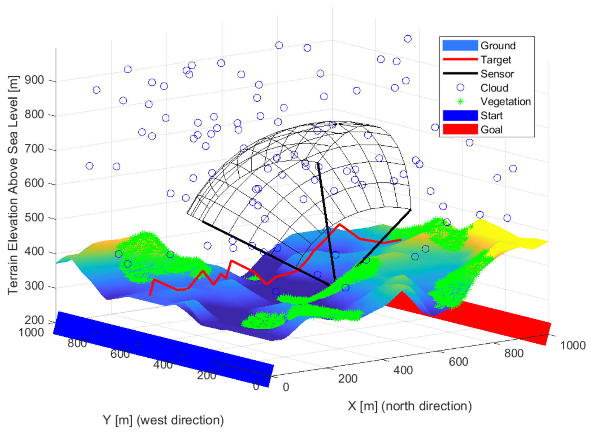
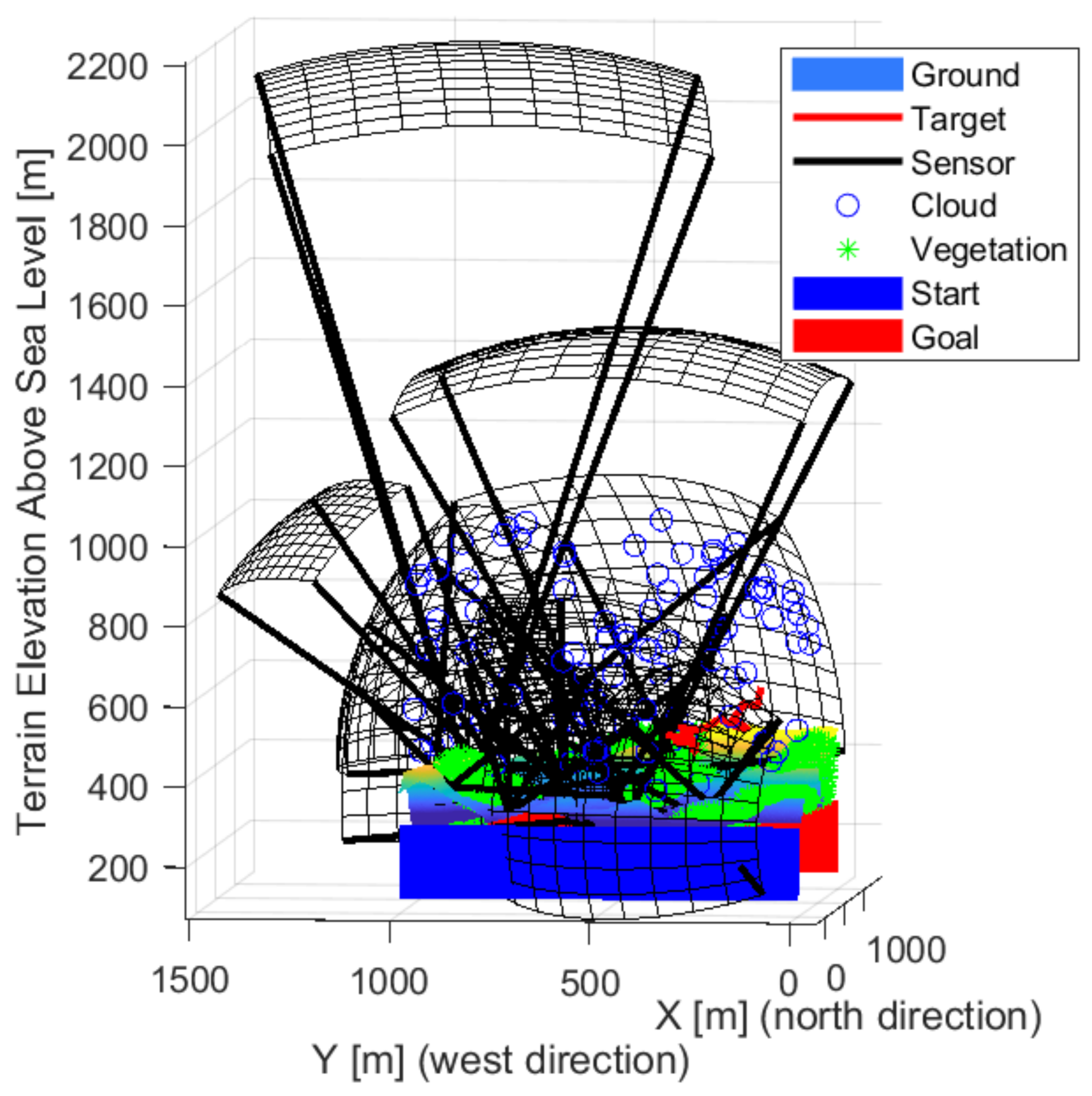
3.1. Environment Model
3.2. Sensor Model
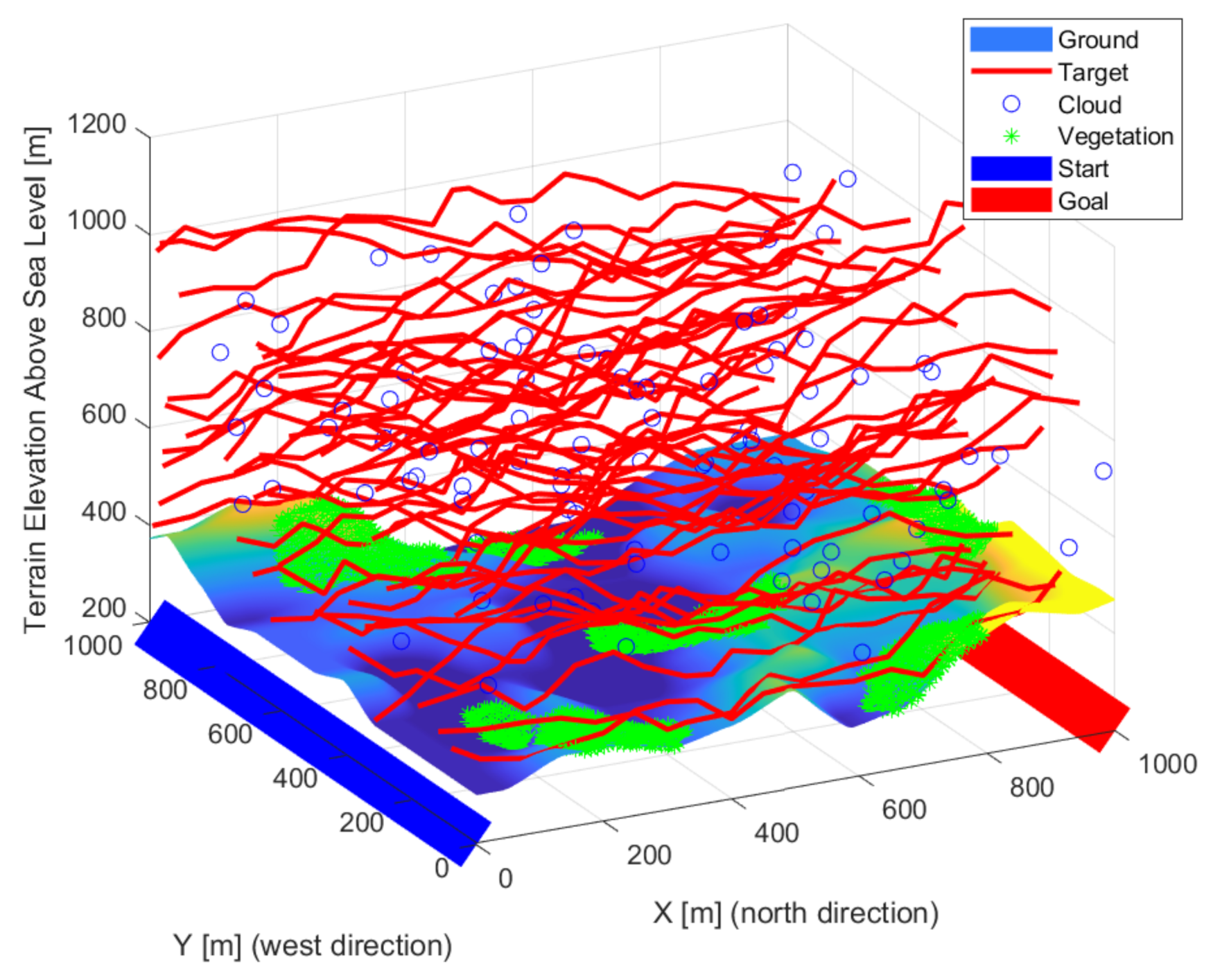
3.3. Target Model
4. Optimization
4.1. Objective
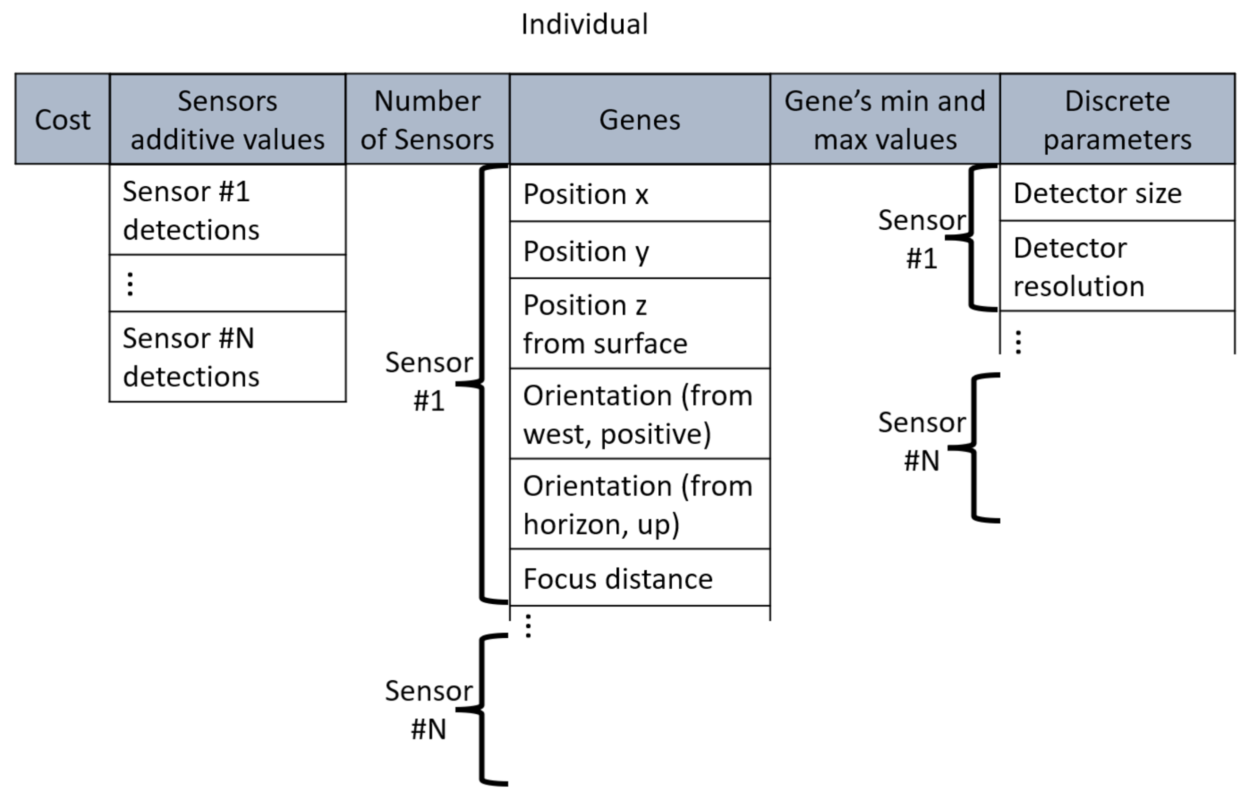
4.2. Individuals
4.3. Optimization Method
| Algorithm 2 Bacterial Evolutionary Algorithm. |
|
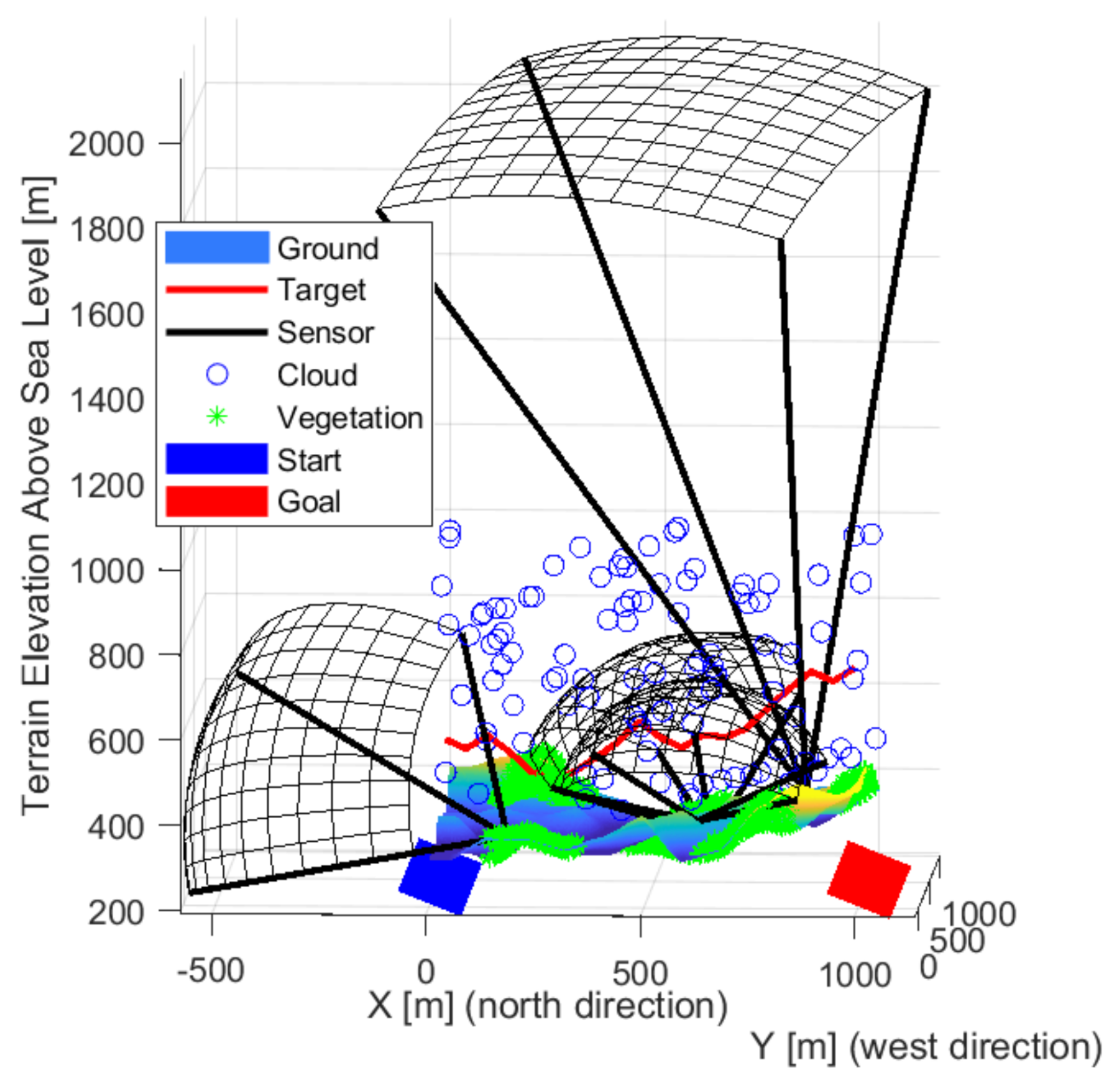
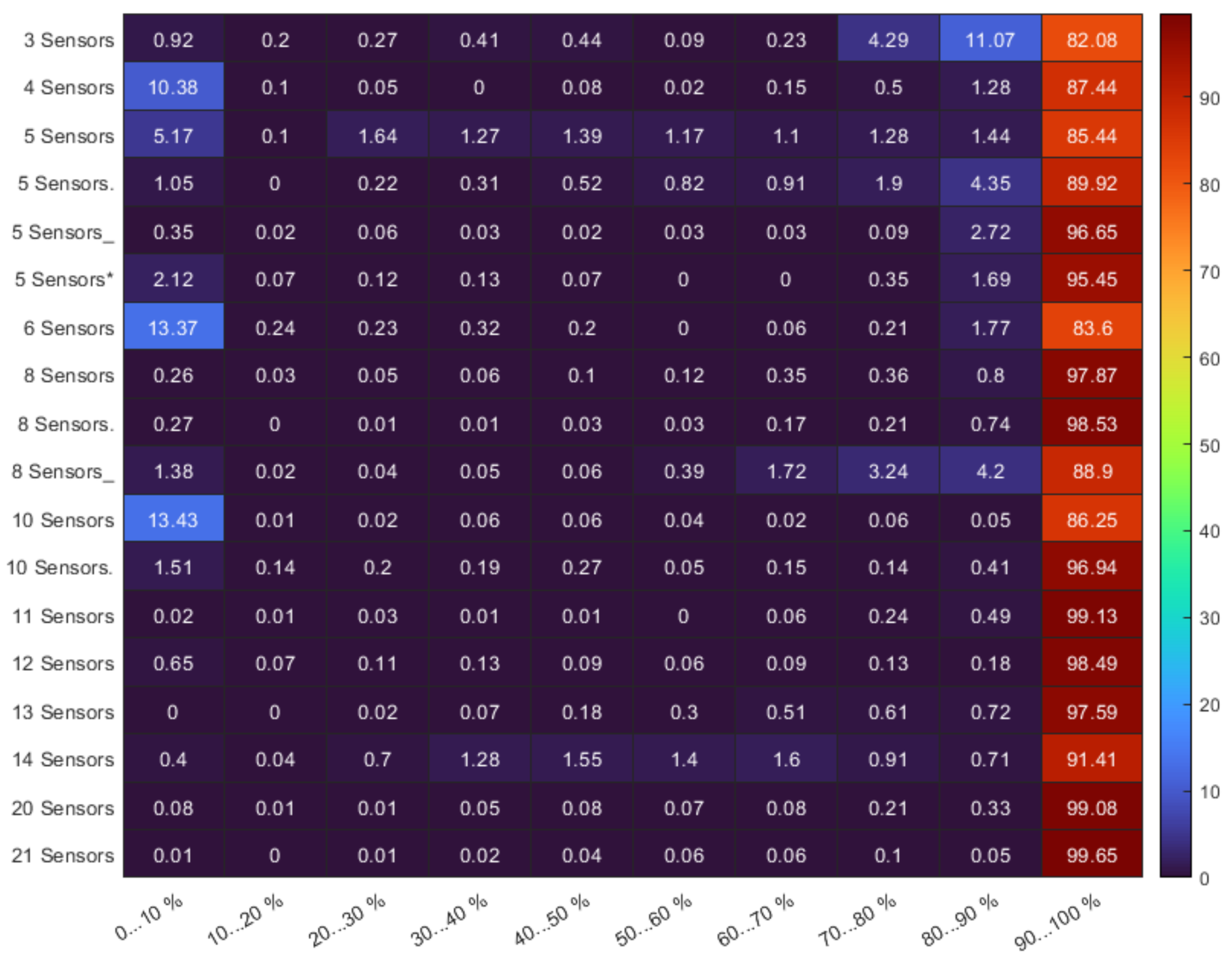
5. Experimental Results
6. Conclusions and Further Work
Author Contributions
Funding
Institutional Review Board Statement
Informed Consent Statement
Conflicts of Interest
References
- Jackman, A. Consumer drone evolutions: Trends, spaces, temporalities, threats. Def. Secur. Anal. 2019, 35, 362–383. [Google Scholar] [CrossRef]
- Yaacoub, J.P.; Noura, H.; Salman, O.; Chehab, A. Security analysis of drones systems: Attacks, limitations, and recommendations. Internet Things 2020, 11, 100218. [Google Scholar] [CrossRef]
- Chamola, V.; Kotesh, P.; Agarwal, A.; Gupta, N.; Guizani, M. A Comprehensive Review of Unmanned Aerial Vehicle Attacks and Neutralization Techniques. Ad Hoc Netw. 2021, 111, 102324. [Google Scholar] [CrossRef] [PubMed]
- EU Research Horizon Projects. Available online: https://frontex.europa.eu/future-of-border-control/eu-research/horizon-projects/ (accessed on 1 January 2022).
- Fedele, R.; Merenda, M. An IoT System for Social Distancing and Emergency Management in Smart Cities Using Multi-Sensor Data. Algorithms 2020, 13, 254. [Google Scholar] [CrossRef]
- Khan, W.; Crockett, K.; O’Shea, J.; Hussain, A.; Khan, B.M. Deception in the eyes of deceiver: A computer vision and machine learning based automated deception detection. Expert Syst. Appl. 2021, 169, 114341. [Google Scholar] [CrossRef]
- Taha, B.; Shoufan, A. Machine Learning-Based Drone Detection and Classification: State-of-the-Art in Research. IEEE Access 2019, 7, 138669–138682. [Google Scholar] [CrossRef]
- Nalamati, M.; Kapoor, A.; Saqib, M.; Sharma, N.; Blumenstein, M. Drone Detection in Long-Range Surveillance Videos. In Proceedings of the 2019 16th IEEE International Conference on Advanced Video and Signal Based Surveillance (AVSS), Taipei, Taiwan, 18–21 September 2019; pp. 1–6. [Google Scholar] [CrossRef]
- Lee, D.H. CNN-based single object detection and tracking in videos and its application to drone detection. Multimed. Tools Appl. 2021, 80, 34237–34248. [Google Scholar] [CrossRef]
- Seidaliyeva, U.; Akhmetov, D.; Ilipbayeva, L.; Matson, E.T. Real-Time and Accurate Drone Detection in a Video with a Static Background. Sensors 2020, 20, 3856. [Google Scholar] [CrossRef]
- Singha, S.; Aydin, B. Automated Drone Detection Using YOLOv4. Drones 2021, 5, 95. [Google Scholar] [CrossRef]
- Jin, R.; Jiang, J.; Qi, Y.; Lin, D.; Song, T. Drone Detection and Pose Estimation Using Relational Graph Networks. Sensors 2019, 19, 1479. [Google Scholar] [CrossRef] [Green Version]
- Behera, D.K.; Bazil Raj, A. Drone Detection and Classification using Deep Learning. In Proceedings of the 2020 4th International Conference on Intelligent Computing and Control Systems (ICICCS), Madurai, India, 13–15 May 2020; pp. 1012–1016. [Google Scholar] [CrossRef]
- Svanström, F.; Englund, C.; Alonso-Fernandez, F. Real-Time Drone Detection and Tracking With Visible, Thermal and Acoustic Sensors. In Proceedings of the 2020 25th International Conference on Pattern Recognition (ICPR), Milan, Italy, 10–15 January 2021; pp. 7265–7272. [Google Scholar] [CrossRef]
- Park, J.; Park, S.; Kim, D.H.; Park, S.O. Leakage Mitigation in Heterodyne FMCW Radar for Small Drone Detection With Stationary Point Concentration Technique. IEEE Trans. Microw. Theory Tech. 2019, 67, 1221–1232. [Google Scholar] [CrossRef] [Green Version]
- Basak, S.; Rajendran, S.; Pollin, S.; Scheers, B. Combined RF-based drone detection and classification. IEEE Trans. Cogn. Commun. Netw. 2021. [Google Scholar] [CrossRef]
- Al-Sa’d, M.F.; Al-Ali, A.; Mohamed, A.; Khattab, T.; Erbad, A. RF-based drone detection and identification using deep learning approaches: An initiative towards a large open source drone database. Future Gener. Comput. Syst. 2019, 100, 86–97. [Google Scholar] [CrossRef]
- Sciancalepore, S.; Ibrahim, O.A.; Oligeri, G.; Di Pietro, R. PiNcH: An effective, efficient, and robust solution to drone detection via network traffic analysis. Comput. Netw. 2020, 168, 107044. [Google Scholar] [CrossRef] [Green Version]
- Anwar, M.Z.; Kaleem, Z.; Jamalipour, A. Machine Learning Inspired Sound-Based Amateur Drone Detection for Public Safety Applications. IEEE Trans. Veh. Technol. 2019, 68, 2526–2534. [Google Scholar] [CrossRef]
- Al-Emadi, S.; Al-Ali, A.; Al-Ali, A. Audio-Based Drone Detection and Identification Using Deep Learning Techniques with Dataset Enhancement through Generative Adversarial Networks. Sensors 2021, 21, 4953. [Google Scholar] [CrossRef]
- Aledhari, M.; Razzak, R.; Parizi, R.M.; Srivastava, G. Sensor Fusion for Drone Detection. In Proceedings of the 2021 IEEE 93rd Vehicular Technology Conference (VTC2021-Spring), Helsinki, Finland, 25–28 April 2021; pp. 1–7. [Google Scholar] [CrossRef]
- Milani, I.; Bongioanni, C.; Colone, F.; Lombardo, P. Fusing active and passive measurements for drone localization. In Proceedings of the 2020 21st International Radar Symposium (IRS), Warsaw, Poland, 5–8 October 2020; pp. 245–249. [Google Scholar] [CrossRef]
- Arjun, D.; Indukala, P.K.; Unnikrishna Menon, K.A. PANCHENDRIYA: A Multi-sensing framework through Wireless Sensor Networks for Advanced Border Surveillance and Human Intruder Detection. In Proceedings of the 2019 International Conference on Communication and Electronics Systems (ICCES), Coimbatore, India, 17–19 July 2019; pp. 295–298. [Google Scholar] [CrossRef]
- Arjun, D.; Indukala, P.; Menon, K.A.U. Integrated Multi-sensor framework for Intruder Detection in Flat Border Area. In Proceedings of the 2019 2nd International Conference on Power and Embedded Drive Control (ICPEDC), Chennai, India, 21–23 August 2019; pp. 557–562. [Google Scholar] [CrossRef]
- Qiao, Y.; Yang, J.; Zhang, Q.; Xi, J.; Kong, L. Multi-UAV Cooperative Patrol Task Planning Novel Method Based on Improved PFIH Algorithm. IEEE Access 2019, 7, 167621–167628. [Google Scholar] [CrossRef]
- Surendonk, T.J.; Chircop, P.A. On the Computational Complexity of the Patrol Boat Scheduling Problem with Complete Coverage. Naval Res. Logist. 2020, 67, 289–299. [Google Scholar] [CrossRef]
- Abushahma, R.I.H.; Ali, M.A.M.; Rahman, N.A.A.; Al-Sanjary, O.I. Comparative Features of Unmanned Aerial Vehicle (UAV) for Border Protection of Libya: A Review. In Proceedings of the 2019 IEEE 15th International Colloquium on Signal Processing Its Applications (CSPA), Penang, Malaysia, 8–9 March 2019; pp. 114–119. [Google Scholar] [CrossRef]
- BorderUAS. Available online: https://frontex.europa.eu/future-of-border-control/eu-research/horizon-projects/borderuas-xFanlJ (accessed on 1 January 2022).
- Dong, Z.; Chang, C.Y.; Chen, G.; Chang, I.H.; Xu, P. Maximizing Surveillance Quality of Boundary Curve in Solar-Powered Wireless Sensor Networks. IEEE Access 2019, 7, 77771–77785. [Google Scholar] [CrossRef]
- Xu, P.; Wu, J.; Shang, C.; Chang, C.Y. GSMS: A Barrier Coverage Algorithm for Joint Surveillance Quality and Network Lifetime in WSNs. IEEE Access 2019, 7, 1. [Google Scholar] [CrossRef]
- Xu, X.; Zhao, C.; Ye, T.; Gu, T. Minimum Cost Deployment of Bistatic Radar Sensor for Perimeter Barrier Coverage. Sensors 2019, 19, 225. [Google Scholar] [CrossRef] [PubMed] [Green Version]
- Liu, Y.; Chin, K.W.; Yang, C.; He, T. Nodes Deployment for Coverage in Rechargeable Wireless Sensor Networks. IEEE Trans. Veh. Technol. 2019, 68, 6064–6073. [Google Scholar] [CrossRef]
- Wang, S.; Yang, X.; Wang, X.; Qian, Z. A Virtual Force Algorithm-Lévy-Embedded Grey Wolf Optimization Algorithm for Wireless Sensor Network Coverage Optimization. Sensors 2019, 19, 2735. [Google Scholar] [CrossRef] [PubMed] [Green Version]
- Akbarzadeh, V.; Gagné, C.; Parizeau, M.; Argany, M.; Mostafavi, M.A. Probabilistic Sensing Model for Sensor Placement Optimization Based on Line-of-Sight Coverage. IEEE Trans. Instrum. Meas. 2013, 62, 293–303. [Google Scholar] [CrossRef]
- Altahir, A.A.; Asirvadam, V.S.; Hamid, N.H.B.; Sebastian, P.; Hassan, M.A.; Saad, N.B.; Ibrahim, R.; Dass, S.C. Visual Sensor Placement Based on Risk Maps. IEEE Trans. Instrum. Meas. 2020, 69, 3109–3117. [Google Scholar] [CrossRef]
- Altahir, A.A.; Asirvadam, V.S.; Sebastian, P.; Hamid, N.H. Solving Surveillance Coverage Demand Based on Dynamic Programming. In Proceedings of the 2020 IEEE Sensors Applications Symposium (SAS), Kuala Lumpur, Malaysia, 9–11 March 2020; pp. 1–6. [Google Scholar] [CrossRef]
- Lanza-Gutiérrez, J.M.; Caballé, N.; Gómez-Pulido, J.A.; Crawford, B.; Soto, R. Toward a Robust Multi-Objective Metaheuristic for Solving the Relay Node Placement Problem in Wireless Sensor Networks. Sensors 2019, 19, 677. [Google Scholar] [CrossRef] [Green Version]
- Tahmasebi, S.; Safi, M.; Zolfi, S.; Maghsoudi, M.R.; Faragardi, H.R.; Fotouhi, H. Cuckoo-PC: An Evolutionary Synchronization-Aware Placement of SDN Controllers for Optimizing the Network Performance in WSNs. Sensors 2020, 20, 3231. [Google Scholar] [CrossRef]
- Thomas, D.; Shankaran, R.; Sheng, Q.; Orgun, M.; Hitchens, M.; Masud, M.; Ni, W.; Mukhopadhyay, S.; Piran, M. QoS-Aware Energy Management and Node Scheduling Schemes for Sensor Network-Based Surveillance Applications. IEEE Access 2020, 9, 3065–3096. [Google Scholar] [CrossRef]
- Zhang, Y.; Liu, M. Regional Optimization Dynamic Algorithm for Node Placement in Wireless Sensor Networks. Sensors 2020, 20, 4216. [Google Scholar] [CrossRef]
- Zaixiu, D.; Shang, C.; Chang, C.Y.; Sinha Roy, D. Barrier Coverage Mechanism Using Adaptive Sensing Range for Renewable WSNs. IEEE Access 2020, 8, 86065–86080. [Google Scholar] [CrossRef]
- Xu, S.; Ou, Y.; Wu, X. Optimal Sensor Placement for 3-D Time-of-Arrival Target Localization. IEEE Trans. Signal Process. 2019, 67, 5018–5031. [Google Scholar] [CrossRef]
- Xu, S. Optimal Sensor Placement for Target Localization Using Hybrid RSS, AOA and TOA Measurements. IEEE Commun. Lett. 2020, 24, 1966–1970. [Google Scholar] [CrossRef]
- Akbarzadeh, V.; Gagné, C.; Parizeau, M. Sensor control for temporal coverage optimization. In Proceedings of the 2016 IEEE Congress on Evolutionary Computation (CEC), Vancouver, BC, Canada, 24–29 July 2016; pp. 4468–4475. [Google Scholar] [CrossRef]
- Zhang, Y.; Liang, R.; Xu, S.; Zhang, L.; Zhang, Y.; Xiao, D. A One-step Pseudolinear Kalman Filter for Invasive Target Tracking in Three-dimensional Space. In Proceedings of the 2021 IEEE International Conference on Real-time Computing and Robotics (RCAR), Xining, China, 15–19 July 2021; pp. 353–358. [Google Scholar] [CrossRef]
- Hu, J.; Zhang, C.; Xu, S.; Chen, C. An Invasive Target Detection and Localization Strategy Using Pan-Tilt-Zoom Cameras for Security Applications. In Proceedings of the 2021 IEEE International Conference on Real-time Computing and Robotics (RCAR), Xining, China, 15–19 July 2021; pp. 1236–1241. [Google Scholar] [CrossRef]
- Wang, S.; Guo, Q.; Xu, S.; Su, D. A Moving Target Detection and Localization Strategy Based on Optical Flow and Pin-hole Imaging Methods Using Monocular Vision. In Proceedings of the 2021 IEEE International Conference on Real-time Computing and Robotics (RCAR), Xining, China, 15–19 July 2021; pp. 147–152. [Google Scholar] [CrossRef]
- Pedrollo, G.; Konzen, A.A.; de Morais, W.O.; Pignaton de Freitas, E. Using Smart Virtual-Sensor Nodes to Improve the Robustness of Indoor Localization Systems. Sensors 2021, 21, 3912. [Google Scholar] [CrossRef]
- De Rainville, F.M.; Mercier, J.P.; Gagné, C.; Giguère, P.; Laurendeau, D. Multisensor placement in 3D environments via visibility estimation and derivative-free optimization. In Proceedings of the 2015 IEEE International Conference on Robotics and Automation (ICRA), Seattle, WA, USA, 26–30 May 2015; pp. 3327–3334. [Google Scholar] [CrossRef]
- Herguedas, R.; López-Nicolás, G.; Sagüés, C. Multi-camera coverage of deformable contour shapes. In Proceedings of the 2019 IEEE 15th International Conference on Automation Science and Engineering (CASE), Vancouver, BC, Canada, 22–26 August 2019; pp. 1597–1602. [Google Scholar] [CrossRef]
- Cuiral-Zueco, I.; López-Nicolás, G. RGB-D Tracking and Optimal Perception of Deformable Objects. IEEE Access 2020, 8, 136884–136897. [Google Scholar] [CrossRef]
- Lee, E.T.; Eun, H.C. Optimal Sensor Placement in Reduced-Order Models Using Modal Constraint Conditions. Sensors 2022, 22, 589. [Google Scholar] [CrossRef]
- Zhang, X.; Zhang, B.; Chen, X.; Fang, Y. Coverage optimization of visual sensor networks for observing 3-D objects: Survey and comparison. Int. J. Intell. Robot. Appl. 2019, 3, 342–361. [Google Scholar] [CrossRef]
- Spielberg, A.; Amini, A.; Chin, L.; Matusik, W.; Rus, D. Co-Learning of Task and Sensor Placement for Soft Robotics. IEEE Robot. Autom. Lett. 2021, 6, 1208–1215. [Google Scholar] [CrossRef]
- Zang, S.; Ding, M.; Smith, D.; Tyler, P.; Rakotoarivelo, T.; Kaafar, M.A. The Impact of Adverse Weather Conditions on Autonomous Vehicles: How Rain, Snow, Fog, and Hail Affect the Performance of a Self-Driving Car. IEEE Veh. Technol. Mag. 2019, 14, 103–111. [Google Scholar] [CrossRef]
- Hasirlioglu, S.; Riener, A. Challenges in Object Detection Under Rainy Weather Conditions. Intelligent Transport Systems, From Research and Development to the Market Uptake; Ferreira, J.C., Martins, A.L., Monteiro, V., Eds.; Springer International Publishing: Cham, Switzerland, 2019; pp. 53–65. [Google Scholar]
- Garg, K.; Nayar, S.K. Vision and Rain. Int. J. Comput. Vis. 2007, 75, 3–27. [Google Scholar] [CrossRef]
- Hasirlioglu, S.; Riener, A. A General Approach for Simulating Rain Effects on Sensor Data in Real and Virtual Environments. IEEE Trans. Intell. Veh. 2020, 5, 426–438. [Google Scholar] [CrossRef]
- Shapiro, F.R. The position of the sun based on a simplified model. Renew. Energy 2022, 184, 176–181. [Google Scholar] [CrossRef]
- Stec, B.; Susek, W. Theory and Measurement of Signal-to-Noise Ratio in Continuous-Wave Noise Radar. Sensors 2018, 18, 1445. [Google Scholar] [CrossRef] [PubMed] [Green Version]
- Wang, Y.; Chu, W.; Fields, S.; Heinemann, C.; Reiter, Z. Detection of Intelligent Intruders in Wireless Sensor Networks. Future Internet 2016, 8, 2. [Google Scholar] [CrossRef]
- Nawa, N.E.; Furuhashi, T. Fuzzy system parameters discovery by bacterial evolutionary algorithm. IEEE Trans. Fuzzy Syst. 1999, 7, 608–616. [Google Scholar] [CrossRef]
- Botzheim, J.; Hámori, B.; Koczy, L.; Ruano, A. Bacterial algorithm applied for fuzzy rule extraction. In Proceedings of the International Conference on Information Processing and Management of Uncertainty in Knowledge-based Systems, Annecy, France, 1–5 July 2002; pp. 1021–1026. [Google Scholar]
- Botzheim, J.; Drobics, M.; Koczy, L. Feature selection using bacterial optimization. In Proceedings of the International Conference on Information Processing and Management of Uncertainty in Knowledge-based Systems, Perugia, Italy, 15–19 June 2004; pp. 797–804. [Google Scholar]
- Das, S.; Chowdhury, A.; Abraham, A. A Bacterial Evolutionary Algorithm for automatic data clustering. In Proceedings of the 2009 IEEE Congress on Evolutionary Computation, Trondheim, Norway, 18–21 May 2009; pp. 2403–2410. [Google Scholar] [CrossRef] [Green Version]
- Luh, G.C.; Lee, S.W. A Bacterial Evolutionary Algorithm for the Job Shop Scheduling Problem. J. Chin. Inst. Ind. Eng. 2006, 23, 185–191. [Google Scholar] [CrossRef]
- Botzheim, J.; Cabrita, C.; Koczy, L.; Ruano, A. Fuzzy Rule Extraction by Bacterial Memetic Algorithms. Int. J. Intell. Syst. 2009, 24, 312–339. [Google Scholar] [CrossRef]
- Bódis, T.; Botzheim, J. Bacterial Memetic Algorithms for Order Picking Routing Problem with Loading Constraints. Expert Syst. Appl. 2018, 105, 196–220. [Google Scholar] [CrossRef]
- Balázs, K.; Botzheim, J.; Koczy, L. Comparative Investigation of Various Evolutionary and Memetic Algorithms; Springer: Berlin/Heidelberg, Germany, 2010; Volume 313, pp. 129–140. [Google Scholar] [CrossRef]
- Zhou, D.; Fang, Y.; Botzheim, J.; Kubota, N.; Liu, H. Bacterial memetic algorithm based feature selection for surface EMG based hand motion recognition in long-term use. In Proceedings of the 2016 IEEE Symposium Series on Computational Intelligence (SSCI), Athens, Greece, 6–9 December 2016; pp. 1–7. [Google Scholar] [CrossRef] [Green Version]
- Kingma, D.P.; Ba, J. Adam: A Method for Stochastic Optimization. 2017. Available online: https://arxiv.org/pdf/1412.6980.pdf (accessed on 1 January 2022).


| Environmental Element | Sign Decrease [%] |
|---|---|
| Clear sky | 0 |
| Clouds | 20 · cloud’s density |
| Ground | [0…50] predefined |
| Walls | [0…50] predefined |
| Vegetation | 50 · vegetation’s density |
Publisher’s Note: MDPI stays neutral with regard to jurisdictional claims in published maps and institutional affiliations. |
© 2022 by the authors. Licensee MDPI, Basel, Switzerland. This article is an open access article distributed under the terms and conditions of the Creative Commons Attribution (CC BY) license (https://creativecommons.org/licenses/by/4.0/).
Share and Cite
Kovács, S.; Bolemányi, B.; Botzheim, J. Placement of Optical Sensors in 3D Terrain Using a Bacterial Evolutionary Algorithm. Sensors 2022, 22, 1161. https://doi.org/10.3390/s22031161
Kovács S, Bolemányi B, Botzheim J. Placement of Optical Sensors in 3D Terrain Using a Bacterial Evolutionary Algorithm. Sensors. 2022; 22(3):1161. https://doi.org/10.3390/s22031161
Chicago/Turabian StyleKovács, Szilárd, Balázs Bolemányi, and János Botzheim. 2022. "Placement of Optical Sensors in 3D Terrain Using a Bacterial Evolutionary Algorithm" Sensors 22, no. 3: 1161. https://doi.org/10.3390/s22031161
APA StyleKovács, S., Bolemányi, B., & Botzheim, J. (2022). Placement of Optical Sensors in 3D Terrain Using a Bacterial Evolutionary Algorithm. Sensors, 22(3), 1161. https://doi.org/10.3390/s22031161