
A Tool for High-Resolution Volumetric Optical Coherence Tomography by Compounding Radial-and Linear Acquired B-Scans Using Registration

 , , , , , ,
Abstract
:1. Introduction
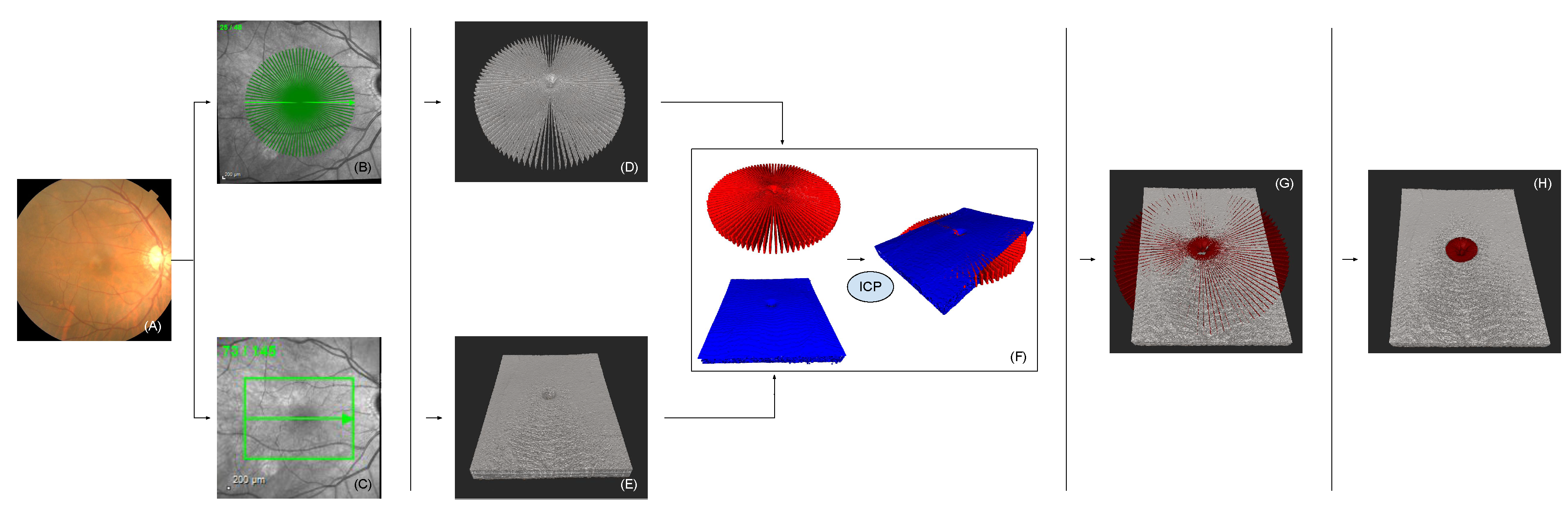
2. Methods
2.1. Linear Volumetric Optical Coherence Tomography
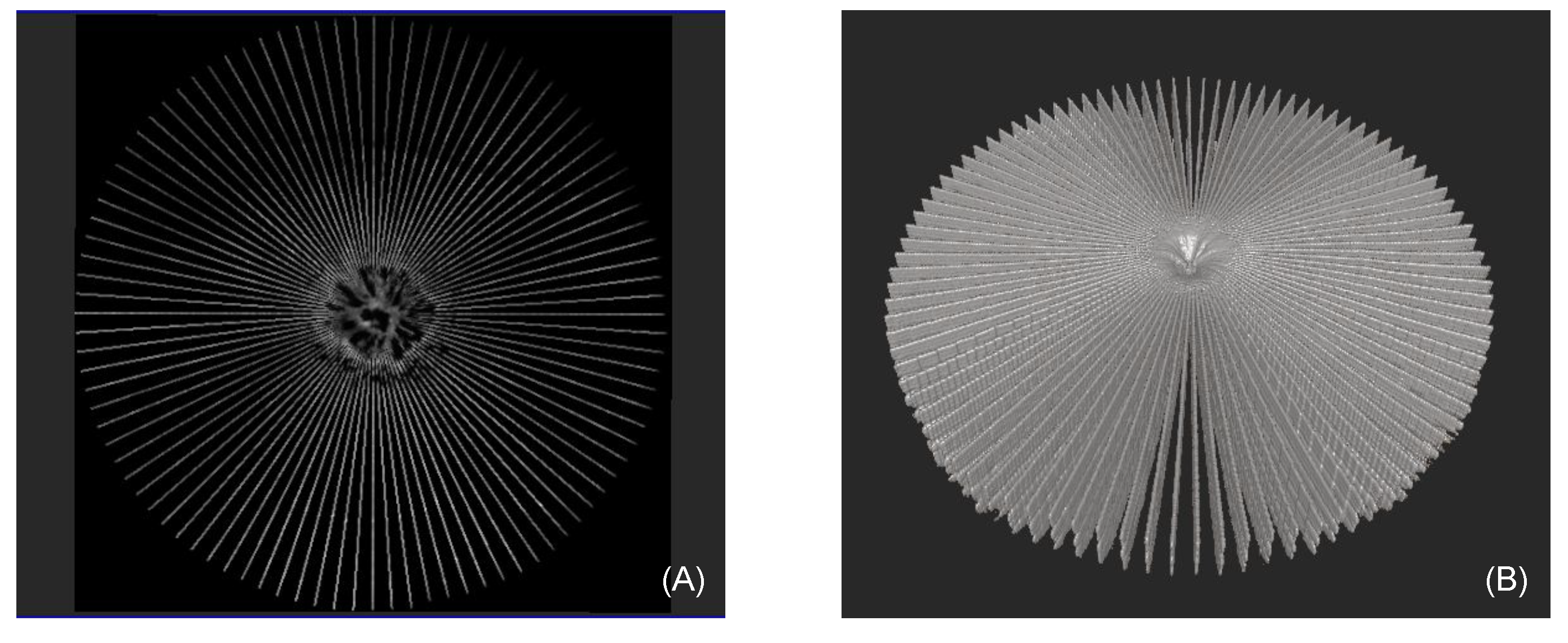
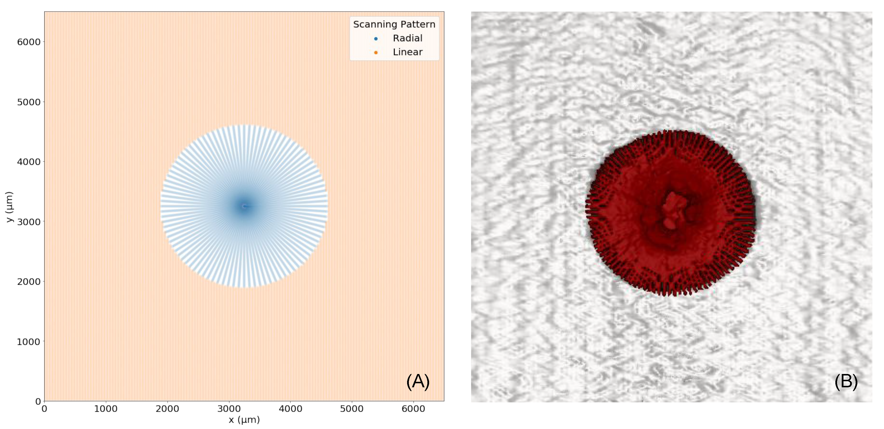
2.2. Radial Volumetric Optical Coherence Tomography
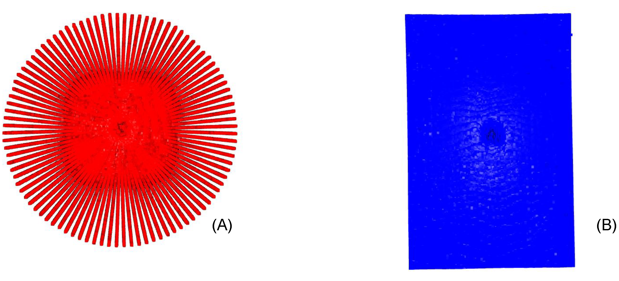
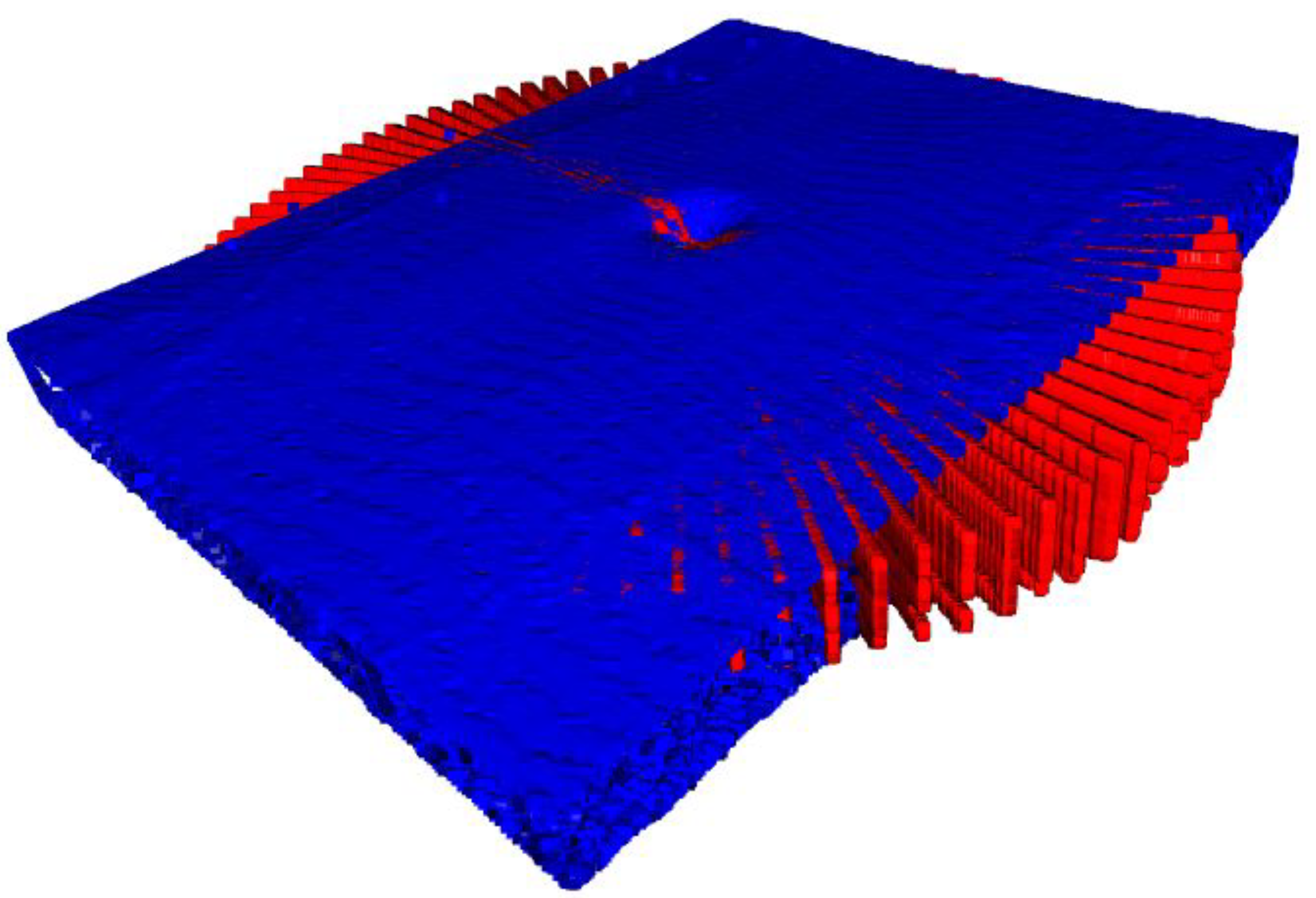
2.3. Iterative Closest Point
2.4. Inflection Point & Compounding
2.5. Enhancement of Spatial A-Scan Resolution
3. Experiments
4. Results
4.1. Radial Volumetric OCT Reconstruction
4.2. Detectability of the Asymmetry of Macular Holes due to 3D reconstruction
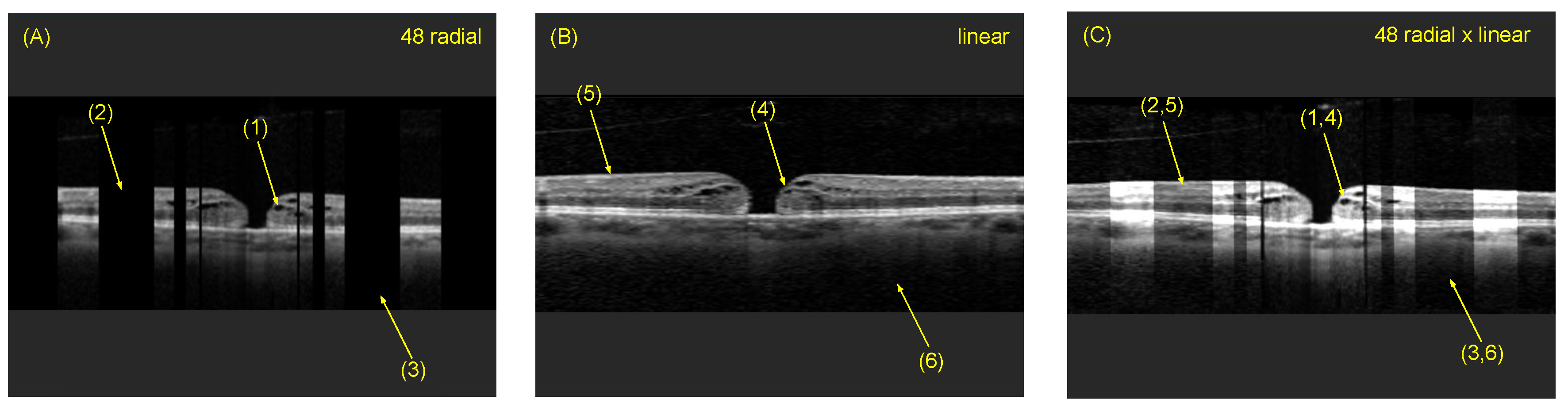
4.3. Comparison of Radial and Fused OCT Reconstruction
4.4. Comparison of Individual B-Scan Slice
4.5. Inflection Point
5. Discussion & Future Work
6. Conclusions
Author Contributions
Funding
Institutional Review Board Statement
Informed Consent Statement
Data Availability Statement
Conflicts of Interest
References
- Huang, D.; Swanson, E.A.; Lin, C.P.; Schuman, J.S.; Stinson, W.G.; Chang, W.; Hee, M.R.; Flotte, T.; Gregory, K.; Puliafito, C.A.; et al. Optical coherence tomography. Science 1991, 254, 1178–1181. [Google Scholar] [CrossRef] [PubMed] [Green Version]
- Swanson, E.A.; Izatt, J.A.; Hee, M.R.; Huang, D.; Lin, C.; Schuman, J.; Puliafito, C.; Fujimoto, J.G. In vivo retinal imaging by optical coherence tomography. Opt. Lett. 1993, 18, 1864–1866. [Google Scholar] [CrossRef] [PubMed]
- Rosenfeld, P.J. Optical coherence tomography and the development of antiangiogenic therapies in neovascular age-related macular degeneration. Investig. Ophthalmol. Vis. Sci. 2016, 57, OCT14–OCT26. [Google Scholar] [CrossRef] [PubMed]
- Spaide, R.F.; Koizumi, H.; Pozonni, M.C. Enhanced depth imaging spectral-domain optical coherence tomography. Am. J. Ophthalmol. 2008, 146, 496–500. [Google Scholar] [CrossRef] [PubMed]
- Nassif, N.; Cense, B.; Park, B.H.; Yun, S.H.; Chen, T.C.; Bouma, B.E.; Tearney, G.J.; de Boer, J.F. In vivo human retinal imaging by ultrahigh-speed spectral domain optical coherence tomography. Opt. Lett. 2004, 29, 480–482. [Google Scholar] [CrossRef] [PubMed] [Green Version]
- Murthy, R.; Haji, S.; Sambhav, K.; Grover, S.; Chalam, K. Clinical applications of spectral domain optical coherence tomography in retinal diseases. Biomed. J. 2016, 39, 107–120. [Google Scholar] [CrossRef] [PubMed] [Green Version]
- Folio, L.S.; Wollstein, G.; Schuman, J.S. Optical coherence tomography: Future trends for imaging in glaucoma. Optom. Vis. Sci. 2012, 89, E554. [Google Scholar] [CrossRef] [PubMed] [Green Version]
- Baumann, C.; Almarzooqi, A.; Blobner, K.; Zapp, D.; Kirchmair, K.; Schwer, L.S.; Lohmann, C.P.; Kaye, S.B. Repeatability and Reproducibility of Macular Hole Size Measurements Using Optical Coherence Tomography. J. Clin. Med. 2021, 10, 2899. [Google Scholar] [CrossRef] [PubMed]
- Chen, Y.; Nasrulloh, A.V.; Wilson, I.; Geenen, C.; Habib, M.; Obara, B.; Steel, D.H. Macular hole morphology and measurement using an automated three-dimensional image segmentation algorithm. BMJ Open Ophthalmol. 2020, 5, e000404. [Google Scholar] [CrossRef] [PubMed]
- Baumann, C.; Iannetta, D.; Sultan, Z.; Pearce, I.A.; Lohmann, C.P.; Zheng, Y.; Kaye, S.B. Predictive association of pre-operative defect areas in the outer retinal layers with visual acuity in macular hole surgery. Transl. Vis. Sci. Technol. 2021, 10, 7. [Google Scholar] [CrossRef] [PubMed]
- Shen, K.; Lu, H.; Baig, S.; Wang, M.R. Improving lateral resolution and image quality of optical coherence tomography by the multi-frame superresolution technique for 3D tissue imaging. Biomed. Opt. Express 2017, 8, 4887–4918. [Google Scholar] [CrossRef] [PubMed] [Green Version]
- Shih, F.Y. Image Processing and Pattern Recognition: Fundamentals and Techniques; John Wiley & Sons: Hoboken, NJ, USA, 2010. [Google Scholar]
- Aumann, S.; Donner, S.; Fischer, J.; Müller, F. Optical Coherence Tomography (OCT): Principle and Technical Realization. In High Resolution Imaging in Microscopy and Ophthalmology: New Frontiers in Biomedical Optics; Springer International Publishing: Cham, Switzerland, 2019; pp. 59–85. [Google Scholar] [CrossRef] [Green Version]
- Lazaridis, G.; Lorenzi, M.; Mohamed-Noriega, J.; Aguilar-Munoa, S.; Suzuki, K.; Nomoto, H.; Ourselin, S.; Garway-Heath, D.F.; Crabb, D.P.; Bunce, C.; et al. OCT signal enhancement with deep learning. Ophthalmol. Glaucoma 2021, 4, 295–304. [Google Scholar] [CrossRef] [PubMed]
- Lebed, E.; Lee, S.; Sarunic, M.V.; Beg, M.F. Rapid radial optical coherence tomography image acquisition. J. Biomed. Opt. 2013, 18, 036004. [Google Scholar] [CrossRef] [PubMed]
- Besl, P.J.; McKay, N.D. Method for registration of 3-D shapes. Sensor fusion IV: Control paradigms and data structures. Int. Soc. Opt. Photonics 1992, 1611, 586–606. [Google Scholar]
- Besl, P.; McKay, N.D. A method for registration of 3-D shapes. IEEE Trans. Pattern Anal. Mach. Intell. 1992, 14, 239–256. [Google Scholar] [CrossRef]
- Chen, Y.; Medioni, G. Object modelling by registration of multiple range images. Image Vis. Comput. 1992, 10, 145–155. [Google Scholar] [CrossRef]
- Benson, S.; Schlottmann, P.; Bunce, C.; Charteris, D. Comparison of macular hole size measured by optical coherence tomography, digital photography, and clinical examination. Eye 2008, 22, 87–90. [Google Scholar] [CrossRef] [PubMed] [Green Version]


Publisher’s Note: MDPI stays neutral with regard to jurisdictional claims in published maps and institutional affiliations. |
© 2022 by the authors. Licensee MDPI, Basel, Switzerland. This article is an open access article distributed under the terms and conditions of the Creative Commons Attribution (CC BY) license (https://creativecommons.org/licenses/by/4.0/).
Share and Cite
Bosch, C.M.; Baumann, C.; Dehghani, S.; Sommersperger, M.; Johannigmann-Malek, N.; Kirchmair, K.; Maier, M.; Nasseri, M.A. A Tool for High-Resolution Volumetric Optical Coherence Tomography by Compounding Radial-and Linear Acquired B-Scans Using Registration. Sensors 2022, 22, 1135. https://doi.org/10.3390/s22031135
Bosch CM, Baumann C, Dehghani S, Sommersperger M, Johannigmann-Malek N, Kirchmair K, Maier M, Nasseri MA. A Tool for High-Resolution Volumetric Optical Coherence Tomography by Compounding Radial-and Linear Acquired B-Scans Using Registration. Sensors. 2022; 22(3):1135. https://doi.org/10.3390/s22031135
Chicago/Turabian StyleBosch, Christian M., Carmen Baumann, Shervin Dehghani, Michael Sommersperger, Navid Johannigmann-Malek, Katharina Kirchmair, Mathias Maier, and Mohammad Ali Nasseri. 2022. "A Tool for High-Resolution Volumetric Optical Coherence Tomography by Compounding Radial-and Linear Acquired B-Scans Using Registration" Sensors 22, no. 3: 1135. https://doi.org/10.3390/s22031135
APA StyleBosch, C. M., Baumann, C., Dehghani, S., Sommersperger, M., Johannigmann-Malek, N., Kirchmair, K., Maier, M., & Nasseri, M. A. (2022). A Tool for High-Resolution Volumetric Optical Coherence Tomography by Compounding Radial-and Linear Acquired B-Scans Using Registration. Sensors, 22(3), 1135. https://doi.org/10.3390/s22031135