
Beyond the Edge: Markerless Pose Estimation of Speech Articulators from Ultrasound and Camera Images Using DeepLabCut

Abstract
:1. Introduction
1.1. State-of-the-Art in Ultrasound Tongue Contour Estimation
1.2. Lip Contour Estimation
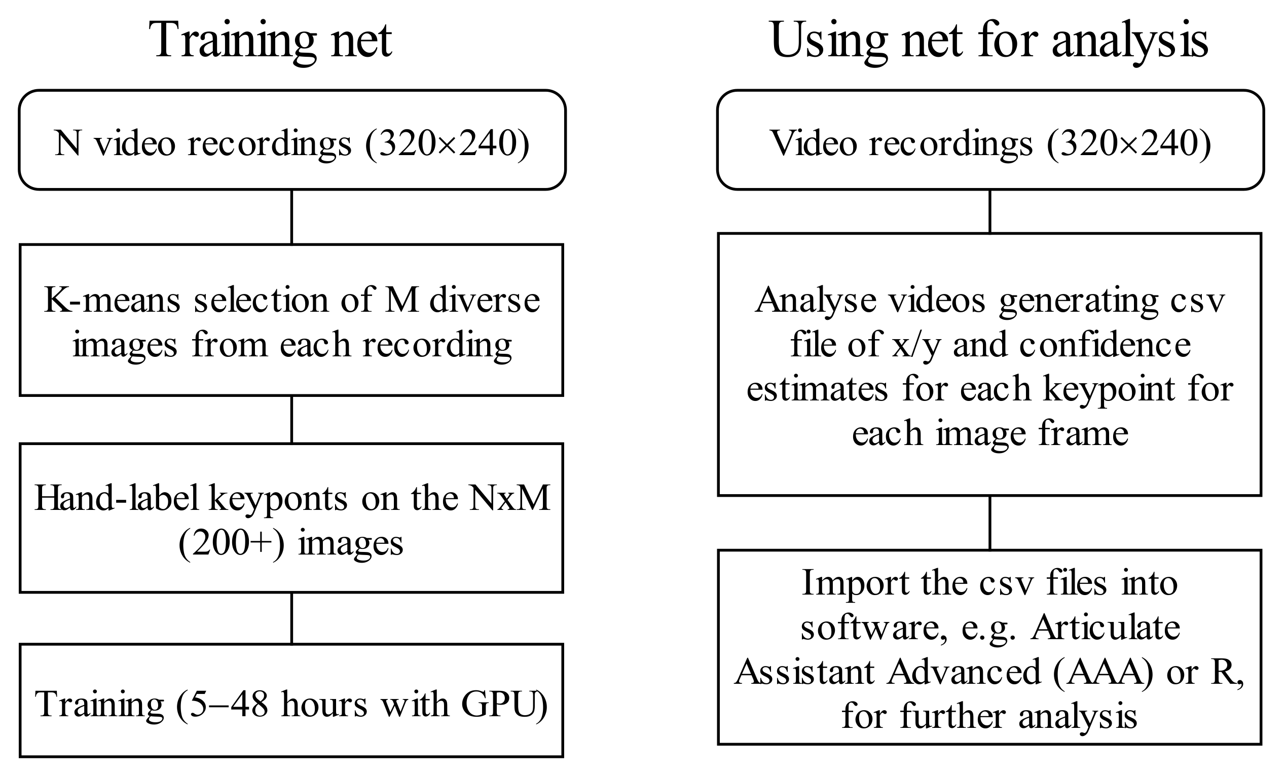
2. Pose Estimation
DeepLabCut
- Shorter training times.
- Less hand-labelled data required for training.
- Robustness on unseen data.
3. Materials and Methods
3.1. Ultrasound Data Preparation
3.1.1. Training Data
- A total of 10 recordings from 6 TaL Corpus [32] adult speakers (Micro system, 90° FOV, 64-element 3 MHz, 20 mm radius convex depth 80, 81 fps). These recordings were the first few recordings from the corpus and not specially selected.
- A total of 4 recordings from 4 UltraSuite corpus [33] Ultrax typically developing children (Ultrasonix RP system, 135° FOV, 128 element 5 MHz 10 mm radius microconvex, depth 80 mm, 121 fps). These were randomly selected. 10 recordings of the authors, using the Micro system with 64-element, 20 mm radius convex probe, and with different field of view and contrast settings
- A total of 2 recordings by Strycharczuk et al. [34] using an EchoB system with a 128-element, 20 mm radius convex probe. These data are from an ultrasound machine not represented in the test set and included to generalize the model.
3.1.2. Test Data
- A total of 10 TaL corpus adult speakers (Articulate Instruments Micro system, 90 FOV, 64-element 3 MHz, 20 mm radius convex depth 80, 81 fps).
- A total of 6 UltraSuite Ultrax typically developing children (Ultrasonix RP system, 135° FOV, 128 element 5 MHz 10 mm radius microconvex, depth 80 mm, 121 fps).
- A total of 2 UltraSuite Ultrax speech sound disordered children (recorded as previous).
- A total of 2 UltraSuite UltraPhonix children with speech sound disorders (SSD) (recorded as previous).
- A total of 2 UltraSuite children with cleft palate repair. Ultrasound (Articulate instruments Micro system, 133° FOV, 64-element 5 MHz, 10 mm radius microconvex, depth 90, 91 fps.
- A total of 3 UltraspeechDataset2017 [35] adults. Ultrasound images (Terason t3000 system, 140° FOV, 128-element, 3–5 MHz 15 mm radius microconvex, depth 70 mm, 60 fps).
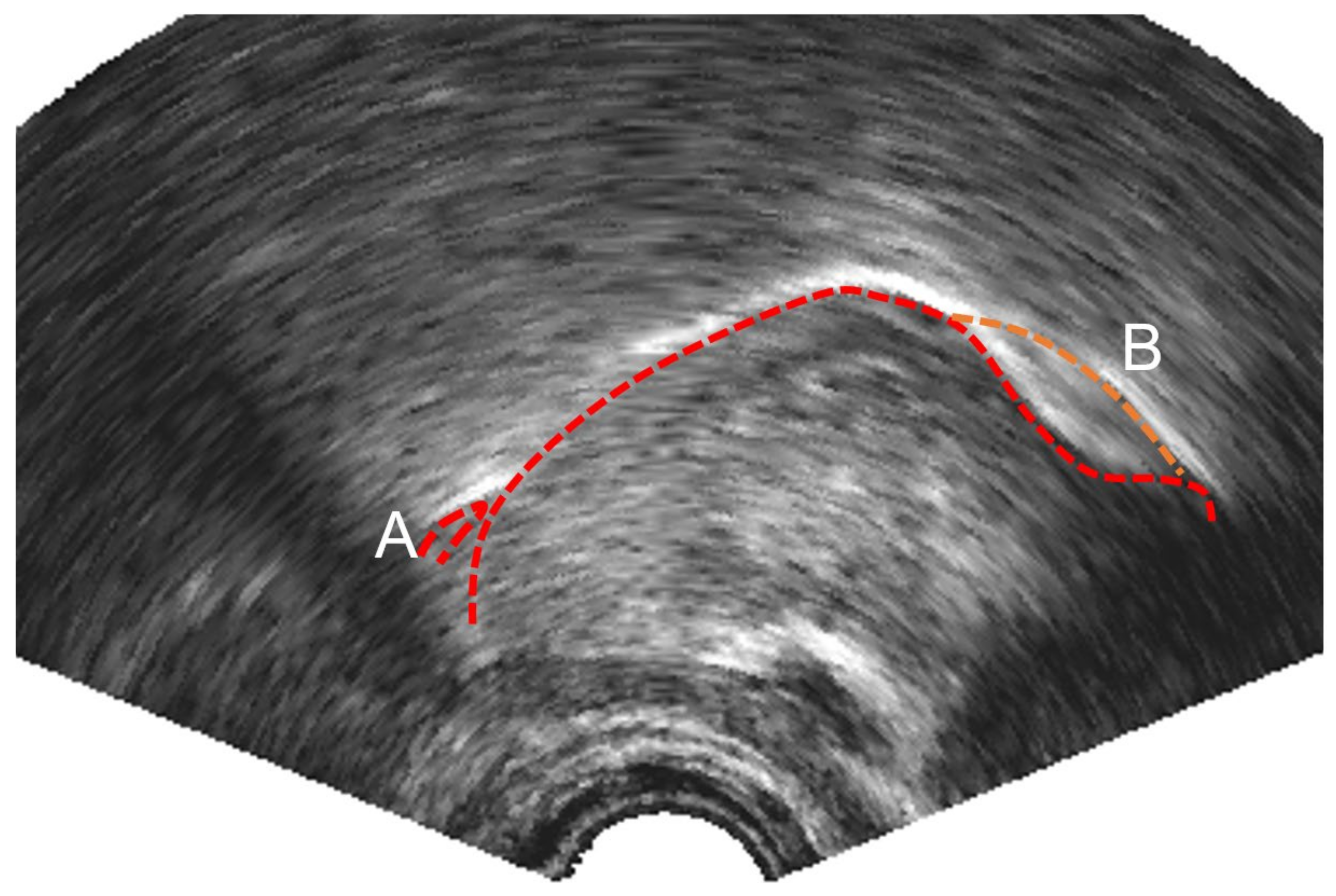
3.1.3. Ultrasound Keypoint Labelling
3.2. EMA-Ultrasound Test Data
3.3. Lip Camera Data Preparation
3.3.1. Training Data
3.3.2. Test Data
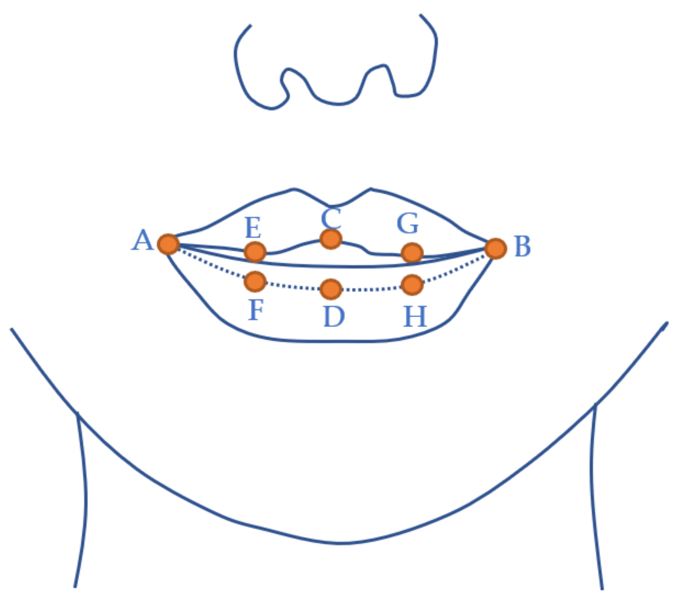
3.3.3. Lip Keypoint Labelling
3.4. Accuracy Measures
3.5. Ultrasound Tongue Contour Estimation Methods
3.5.1. DLC Ultrasound
3.5.2. SLURP
- Colormap = “gray”, Sigma = 5.0, Delta = 2.0, Band Penalty = 2.0, Alpha = 0.80,
- Lambda = 0.95, Adaptive Sampling = Enabled, Particles = Min 10, Max 1000.
3.5.3. MTracker
3.5.4. DeepEdge
3.6. Method for Comparing EMA Position Sensors to DLC Keypoints
3.7. Method for Evaluating DLC Performance on Lip Camera Data
4. Results
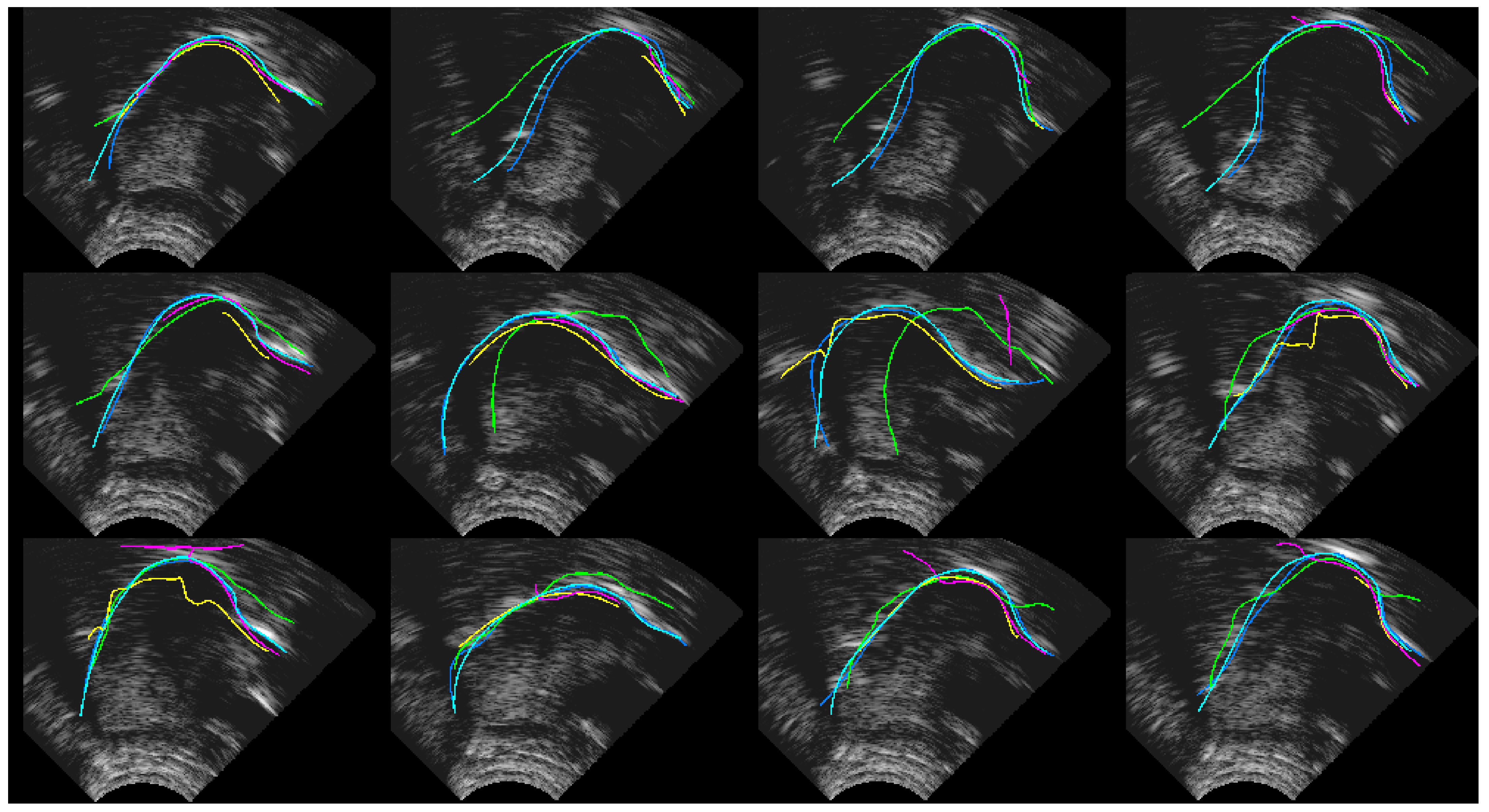
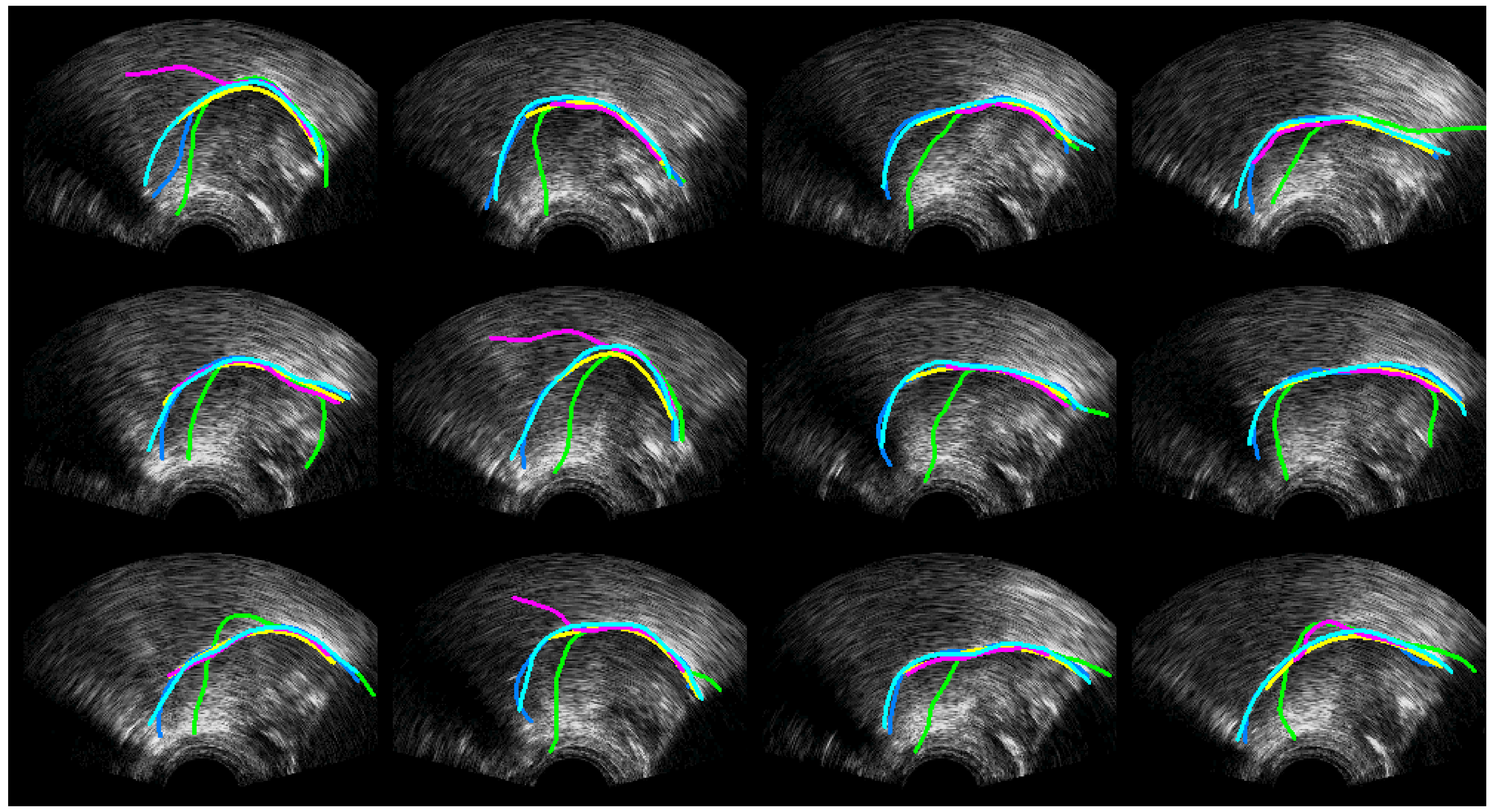
4.1. Ultrasound Contour Tracking
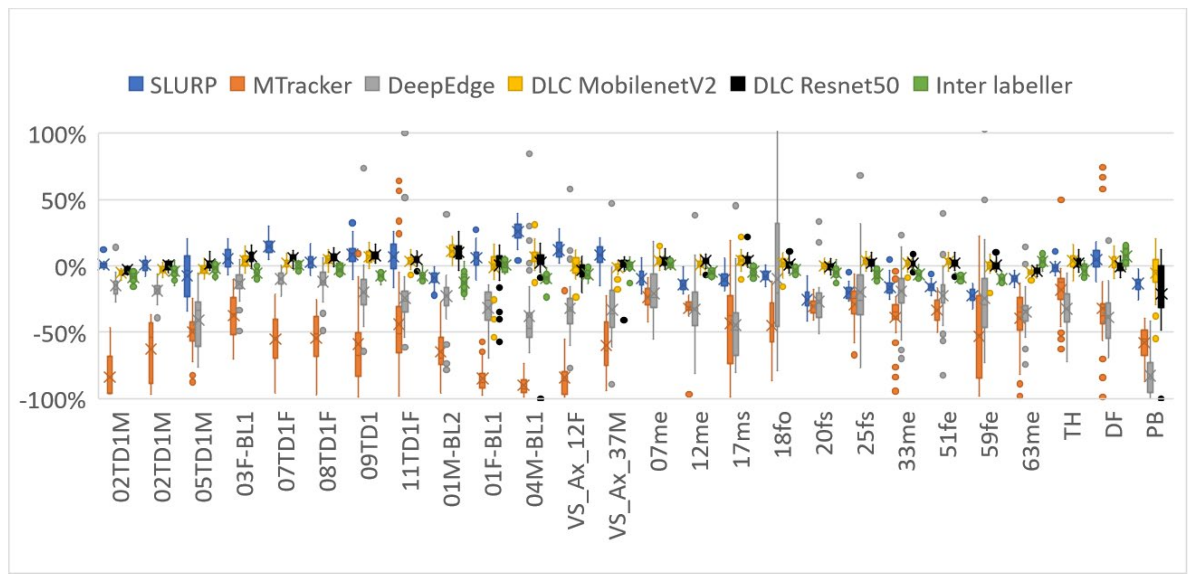
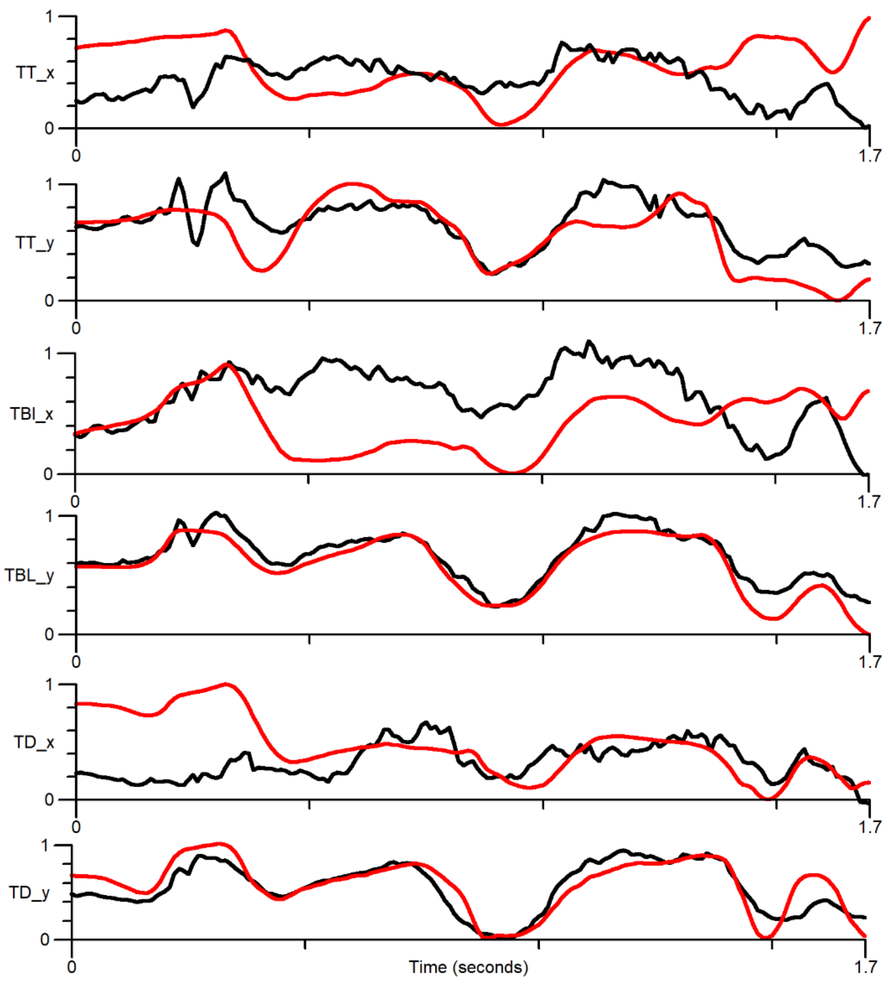
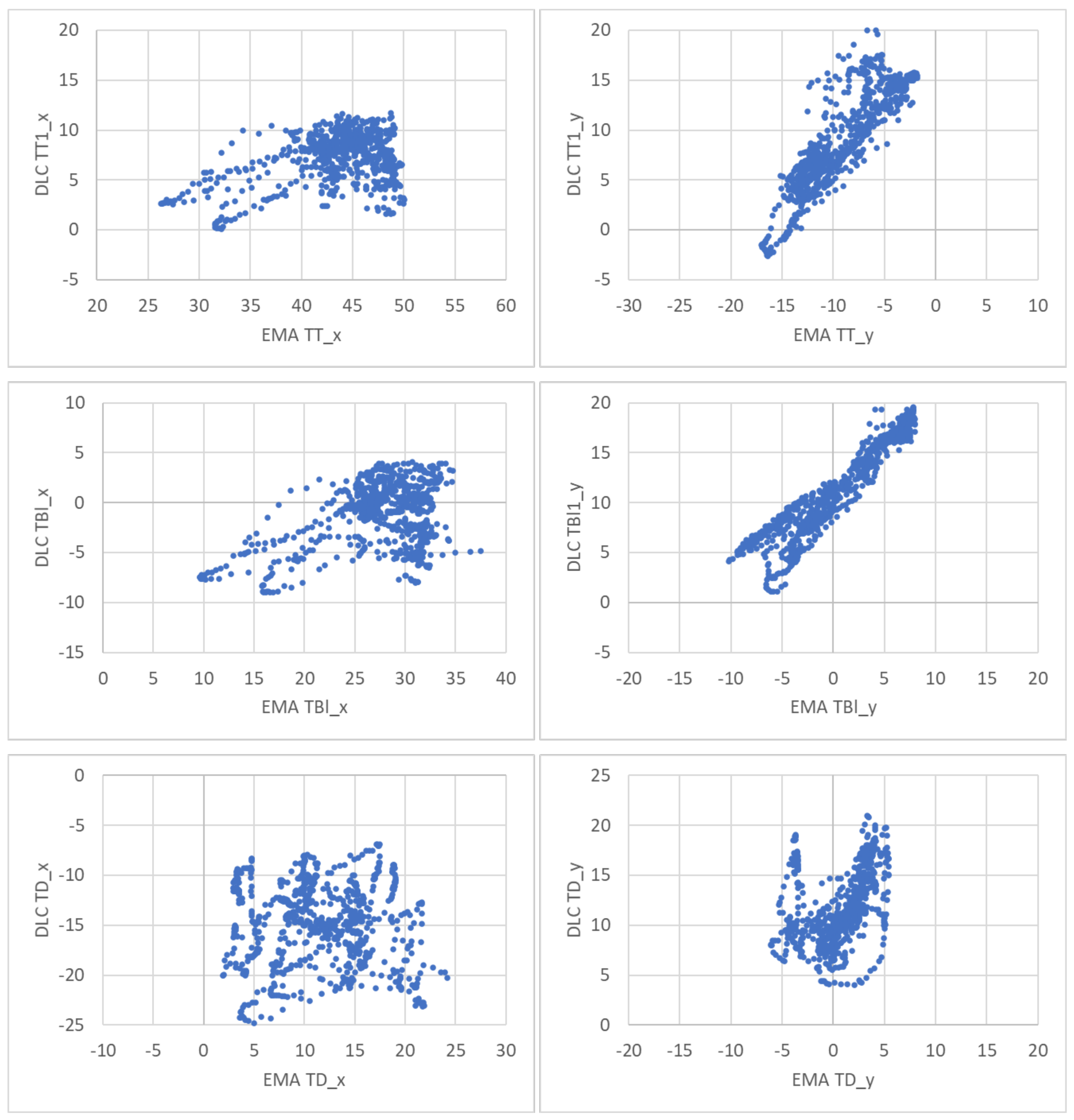
4.2. Ultrasound-EMA Point Tracking
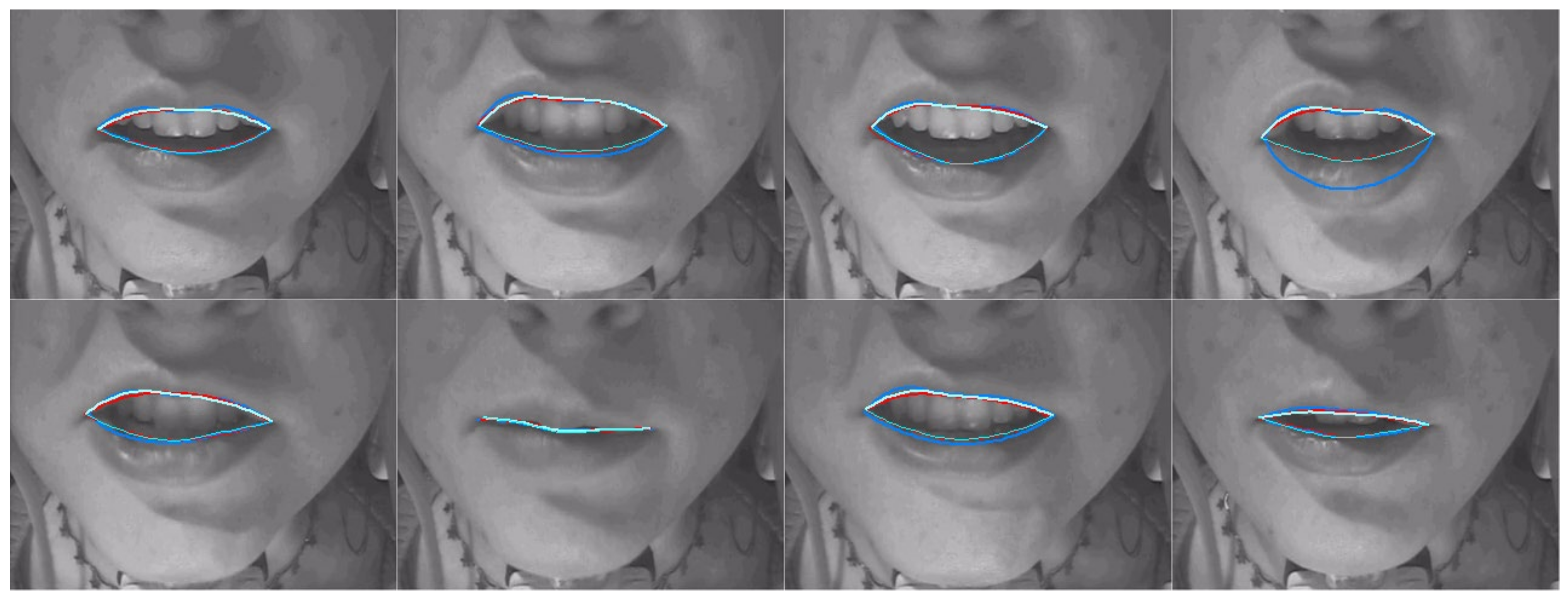
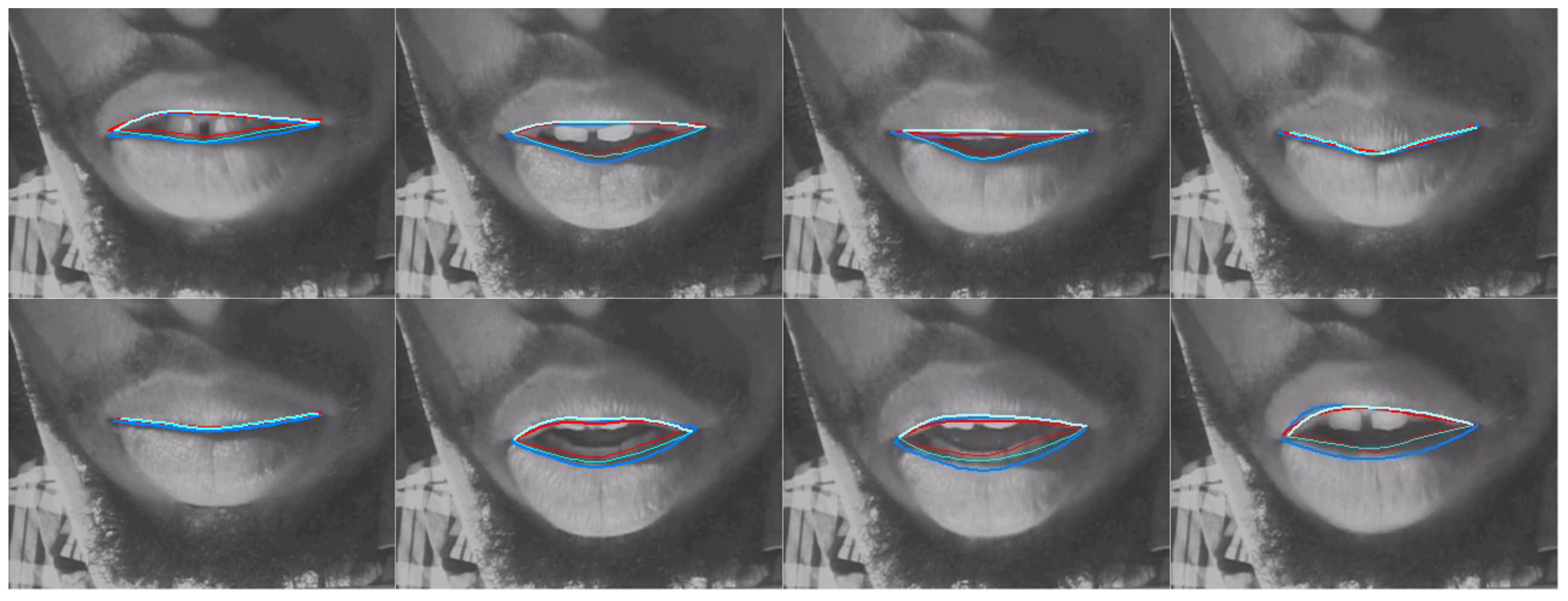
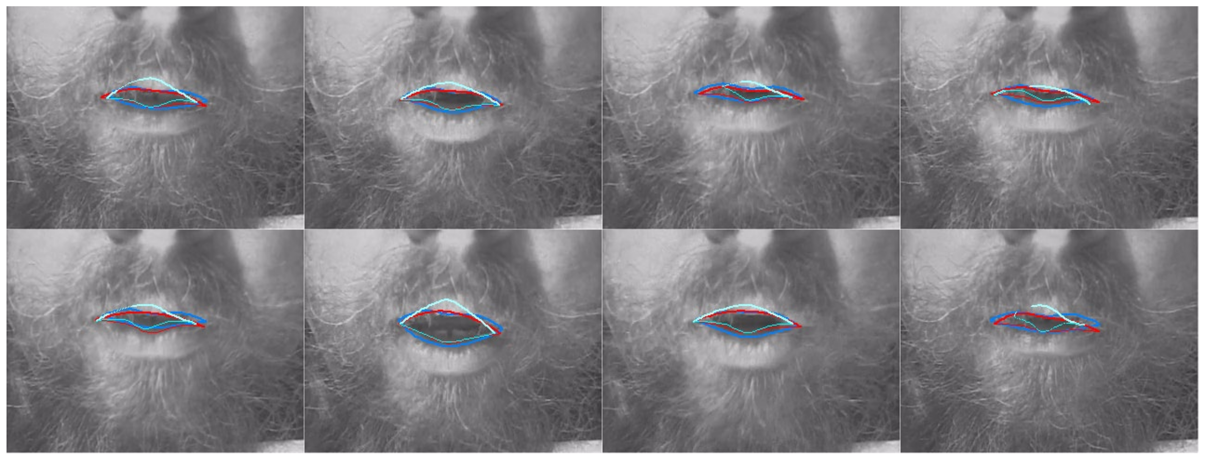
4.3. Camera Lip Tracking
5. Discussion
- Pose estimation is capable of learning how to label features that do not necessarily correspond to edges.
- Pose estimation can estimate feature positions to the same level of accuracy as a human labeller.
Supplementary Materials
Author Contributions
Funding
Institutional Review Board Statement
Informed Consent Statement
Data Availability Statement
Acknowledgments
Conflicts of Interest
Appendix A
Appendix B

References
- Fuchs, S.; Perrier, P. On the complex nature of speech kinematics. ZAS Pap. Linguist. 2005, 42, 137–165. [Google Scholar] [CrossRef]
- Kass, M.; Witkin, A.; Terzopoulos, D. Snakes: Active contour models. Int. J. Comput. Vis. 1988, 1, 321–331. [Google Scholar] [CrossRef]
- Li, M.; Kambhamettu, C.; Stone, M. Automatic contour tracking in ultrasound images. Clin. Linguist. Phon. 2005, 19, 545–554. [Google Scholar] [CrossRef] [PubMed]
- Csapó, T.G.; Lulich, S.M. Error analysis of extracted tongue contours from 2D ultrasound images. In Proceedings of the Sixteenth Annual Conference of the International Speech Communication Association, Dresden, Germany, 6–10 September 2015. [Google Scholar]
- Laporte, C.; Ménard, L. Multi-hypothesis tracking of the tongue surface in ultrasound video recordings of normal and impaired speech. Med. Image Anal. 2018, 44, 98–114. [Google Scholar] [CrossRef]
- Fasel, I.; Berry, J. Deep belief networks for real-time extraction of tongue contours from ultrasound during speech. In Proceedings of the 2010 20th International Conference on Pattern Recognition, Istanbul, Turkey, 23–26 August 2010; pp. 1493–1496. [Google Scholar]
- Fabre, D.; Hueber, T.; Bocquelet, F.; Badin, P. Tongue tracking in ultrasound images using eigentongue decomposition and artificial neural networks. In Proceedings of the 16th Annual Conference of the International Speech Communication Association (Interspeech 2015), Dresden, Germany, 6–10 September 2015. [Google Scholar]
- Xu, K.; Gábor Csapó, T.; Roussel, P.; Denby, B. A comparative study on the contour tracking algorithms in ultrasound tongue images with automatic re-initialization. J. Acoust. Soc. Am. 2016, 139, EL154–EL160. [Google Scholar] [CrossRef] [Green Version]
- Mozaffari, M.H.; Yamane, N.; Lee, W. Deep Learning for Automatic Tracking of Tongue Surface in Real-time Ultrasound Videos, Landmarks instead of Contours. In Proceedings of the 2020 IEEE International Conference on Bioinformatics and Biomedicine (BIBM), Seoul, Korea, 16–19 December 2020; pp. 2785–2792. [Google Scholar]
- Aslan, E.; Akgul, Y.S. Tongue Contour Tracking in Ultrasound Images with Spatiotemporal LSTM Networks. In Proceedings of the German Conference on Pattern Recognition, Dortmund, Germany, 10–13 September 2019; pp. 513–521. [Google Scholar]
- Zhu, J.; Styler, W.; Calloway, I. A CNN-based tool for automatic tongue contour tracking in ultrasound images. arXiv, 2019; arXiv:1907.10210. [Google Scholar]
- Chen, W.; Tiede, M.; Whalen, D.H. DeepEdge: Automatic Ultrasound Tongue Contouring Combining a Deep Neural Network and an Edge Detection Algorithm. 2020. Available online: https://issp2020.yale.edu/S05/chen_05_16_161_poster.pdf (accessed on 5 February 2021).
- Ronneberger, O.; Fischer, P.; Brox, T. U-net: Convolutional networks for biomedical image segmentation. In Proceedings of the International Conference on Medical Image Computing and Computer-Assisted Intervention, Munich, Germany, 5–9 October 2015; pp. 234–241. [Google Scholar]
- Tang, L.; Bressmann, T.; Hamarneh, G. Tongue contour tracking in dynamic ultrasound via higher-order MRFs and efficient fusion moves. Med. Image Anal. 2012, 16, 1503–1520. [Google Scholar] [CrossRef]
- Jaumard-Hakoun, A.; Xu, K.; Roussel-Ragot, P.; Dreyfus, G.; Denby, B. Tongue contour extraction from ultrasound images based on deep neural network. arXiv, 2016; arXiv:1605.05912. [Google Scholar]
- Chiou, G.I.; Hwang, J. Lipreading from color video. IEEE Trans. Image Process. 1997, 6, 1192–1195. [Google Scholar] [CrossRef]
- Luettin, J.; Thacker, N.A.; Beet, S.W. Speechreading using shape and intensity information. In Proceedings of the Fourth International Conference on Spoken Language Processing, ICSLP’96, Philadelphia, PA, USA, 3–6 October 1996; pp. 58–61. [Google Scholar]
- Kaucic, R.; Dalton, B.; Blake, A. Real-time lip tracking for audio-visual speech recognition applications. In Proceedings of the European Conference on Computer Vision, Cambridge, UK, 15–18 April 1996; pp. 376–387. [Google Scholar]
- Lallouache, M.T. Un Poste“ Visage-Parole” Couleur: Acquisition et Traitement Automatique des Contours des Lèvres. Ph.D. Thesis, INPG, Grenoble, France, 1991. [Google Scholar]
- King, H.; Ferragne, E. Labiodentals /r/ here to stay: Deep learning shows us why. Anglophonia Fr. J. Engl. Linguist. 2020, 30. [Google Scholar] [CrossRef]
- Mathis, M.W.; Mathis, A. Deep learning tools for the measurement of animal behavior in neuroscience. Curr. Opin. Neurobiol. 2020, 60, 1–11. [Google Scholar] [CrossRef] [PubMed]
- Mathis, A.; Mamidanna, P.; Cury, K.M.; Abe, T.; Murthy, V.N.; Mathis, M.W.; Bethge, M. DeepLabCut: Markerless pose estimation of user-defined body parts with deep learning. Nat. Neurosci. 2018, 21, 1281–1289. [Google Scholar] [CrossRef] [PubMed]
- Graving, J.M.; Chae, D.; Naik, H.; Li, L.; Koger, B.; Costelloe, B.R.; Couzin, I.D. DeepPoseKit, a software toolkit for fast and robust animal pose estimation using deep learning. eLife 2019, 8, e47994. [Google Scholar] [CrossRef]
- Pereira, T.D.; Tabris, N.; Li, J.; Ravindranath, S.; Papadoyannis, E.S.; Wang, Z.Y.; Turner, D.M.; McKenzie-Smith, G.; Kocher, S.D.; Falkner, A.L. SLEAP: Multi-animal pose tracking. bioRxiv 2020. [Google Scholar] [CrossRef]
- Mathis, A.; Biasi, T.; Schneider, S.; Yuksekgonul, M.; Rogers, B.; Bethge, M.; Mathis, M.W. Pretraining boosts out-of-domain robustness for pose estimation. In Proceedings of the IEEE/CVF Winter Conference on Applications of Computer Vision, Virtual Conference, 5–9 January 2021; pp. 1859–1868. [Google Scholar]
- Johnston, B.; de Chazal, P. A review of image-based automatic facial landmark identification techniques. EURASIP J. Image Video Process. 2018, 2018, 1–23. [Google Scholar] [CrossRef] [Green Version]
- Andriluka, M.; Pishchulin, L.; Gehler, P.; Schiele, B. 2D Human Pose Estimation: New Benchmark and State of the Art Analysis. In Proceedings of the IEEE Conference on Computer Vision and Pattern Recognition (CVPR), Columbus, OH, USA, 24–27 June 2014; pp. 3686–3693. [Google Scholar]
- Sandler, M.; Howard, A.; Zhu, M.; Zhmoginov, A.; Chen, L. MobileNetV2: Inverted residuals and linear bottlenecks. In Proceedings of the IEEE Conference on Computer Vision and Pattern Recognition, Salt Lake City, UT, USA, 18–22 June 2018; pp. 4510–4520. [Google Scholar]
- He, K.; Zhang, X.; Ren, S.; Sun, J. Deep residual learning for image recognition. In Proceedings of the IEEE Conference on Computer Vision and Pattern Recognition, Las Vegas, NV, USA, 26 June–1 July 2016; pp. 770–778. [Google Scholar]
- Tan, M.; Le, Q. Efficientnet: Rethinking model scaling for convolutional neural networks. In Proceedings of the International Conference on Machine Learning PMLR, Long Beach, CA, USA, 9–15 June 2019; Volume 97, pp. 6105–6114. [Google Scholar]
- Insafutdinov, E.; Pishchulin, L.; Andres, B.; Andriluka, M.; Schiele, B. DeeperCut: A Deeper, Stronger, and Faster Multi-person Pose Estimation Model. In Computer Vision—ECCV 2016; Springer International Publishing: Cham, Switzerland, 2016; pp. 34–50. [Google Scholar]
- Ribeiro, M.S.; Sanger, J.; Zhang, J.; Eshky, A.; Wrench, A.; Richmond, K.; Renals, S. TaL: A synchronised multi-speaker corpus of ultrasound tongue imaging, audio, and lip videos. In Proceedings of the 2021 IEEE Spoken Language Technology Workshop (SLT), Shenzhen, China, 19–22 January 2021; pp. 1109–1116. [Google Scholar]
- Eshky, A.; Ribeiro, M.S.; Cleland, J.; Richmond, K.; Roxburgh, Z.; Scobbie, J.; Wrench, A. UltraSuite: A repository of ultrasound and acoustic data from child speech therapy sessions. arXiv, 2019; arXiv:1907.00835. [Google Scholar]
- Strycharczuk, P.; Ćavar, M.; Coretta, S. Distance vs time. Acoustic and articulatory consequences of reduced vowel duration in Polish. J. Acoust. Soc. Am. 2021, 150, 592–607. [Google Scholar] [CrossRef]
- Fabre, D.; Hueber, T.; Girin, L.; Alameda-Pineda, X.; Badin, P. Automatic animation of an articulatory tongue model from ultrasound images of the vocal tract. Speech Commun. 2017, 93, 63–75. [Google Scholar] [CrossRef]
- Nath, T.; Mathis, A.; Chen, A.C.; Patel, A.; Bethge, M.; Mathis, M.W. Using DeepLabCut for 3D markerless pose estimation across species and behaviors. Nat. Protoc. 2019, 14, 2152–2176. [Google Scholar] [CrossRef]
- GetContours V3.5. Available online: https://github.com/mktiede/GetContours (accessed on 21 July 2021).
- Scobbie, J.M.; Lawson, E.; Cowen, S.; Cleland, J.; Wrench, A.A. A Common Co-Ordinate System for Mid-Sagittal Articulatory Measurement. QMU CASL Working Papers WP-20. 2011. Available online: https://eresearch.qmu.ac.uk/handle/20.500.12289/3597 (accessed on 28 November 2021).
- Eslami, M.; Neuschaefer-Rube, C.; Serrurier, A. Automatic vocal tract landmark localization from midsagittal MRI data. Sci. Rep. 2020, 10, 1–13. [Google Scholar] [CrossRef] [Green Version]
- Lim, Y.; Toutios, A.; Bliesener, Y.; Tian, Y.; Lingala, S.G.; Vaz, C.; Sorensen, T.; Oh, M.; Harper, S.; Chen, W. A multispeaker dataset of raw and reconstructed speech production real-time MRI video and 3D volumetric images. arXiv, 2021; arXiv:2102.07896. [Google Scholar] [CrossRef] [PubMed]


| Algorithm | MSD (Mean/s.d.) mm |
|---|---|
| EdgeTrak 1 | 6.8/3.9 |
| SLURP 1 | 1.7/1.1 |
| TongueTrack 1 | 3.5/1.5 |
| AutoTrace 1,2 | 2.6/1.2 |
| DeepEdge (NN + Snake) 3 | 1.4/1.4 |
| MTracker 4 | 1.4/0.7 |
| BowNet 5 | 3.9/- |
| TongueNet 5 | 3.1/- |
| IrisNet 5 | 2.7/- |
| Human-human | 0.9 6/-, 1.3 7 |
| Algorithm | Frames per Second 1 (GPU/CPU) | Image Size | Training Data/Time (Frames/Hours) |
|---|---|---|---|
| SLURP 2,3 | NA/8.5 | data | N/A |
| DeepEdge (NN + Snake) | 2.7/NA | 64 × 64 | 2700/2 |
| DeepEdge (NN only) | 3.0/NA | 64 × 64 | 2700/2 |
| MTracker | 27/NA | 128 × 128 | 35,160/2 |
| DeepLabCut (MobNetV2_1.0) | 287/7.3 4 | 320 × 240 | 520/7.5 |
| DeepLabCut (ResNet50) | 157/4.0 4 | 320 × 240 | 520/16 |
| DeepLabCut (ResNet101) | 105/2.6 4 | 320 × 240 | 520/30 |
| DeepLabCut (EfficientNet B6) | 27/1.7 4 | 320 × 240 | 520/48 |
| MobileNetV2 Training Data | MSD (Mean, s.d., Median) | MSD p Value 1 | %Length Diff (Mean, s.d., Median) |
|---|---|---|---|
| conf 80% 520 frames | 1.06, 0.59, 0.90 | 1.00 | +1.8, 7.0, +2.0 |
| 1.06, 0.71, 0.89 | 0.89 | +1.8, 9.1, +1.8 | |
| conf 80% 390 frames | 1.12, 0.86, 0.91 | 0.09 | +2.8, 10.7, +2.5 |
| conf 80% 260 frames | 1.13, 0.71, 0.94 | 0.03 | +1.9, 9.7, +1.7 |
| conf 80% 130 frames | 1.17, 0.79, 0.94 | <0.001 | +3.5, 8.1, +3.2 |
| Algorithm | MSD (Mean, s.d., Median) | MSD p Values 1 | %Length Diff (Mean, s.d., Median) |
|---|---|---|---|
| SLURP | 2.3, 1.5, 1.9 | <0.001 | −3.8, 14.4, −4.6 |
| DeepEdge (NN only) | 2.8, 3.1, 1.9 | <0.001 | −27.5, 25.3, −26.0 |
| MTracker | 3.2, 5.8, 1.5 | <0.001 | −49.0, 28.7, −44.4 |
| DLC (MobileNetV2_1.0 conf 80%) | 1.06, 0.59, 0.90 | 0.04 | +1.8, 7.0, +2.0 |
| DLC (ResNet50 conf 80%) | 0.93, 0.46, 0.82 | 0.29 | +1.6, 8.8, +2.2 |
| DLC (ResNet101 conf 80%) | 0.96, 0.67, 0.81 | 0.80 | +1.8, 9.1, +1.8 |
| Inter-labeller | 0.96, 0.39, 0.88 | 1.0 | −4.3, 6.2, −4.8 |
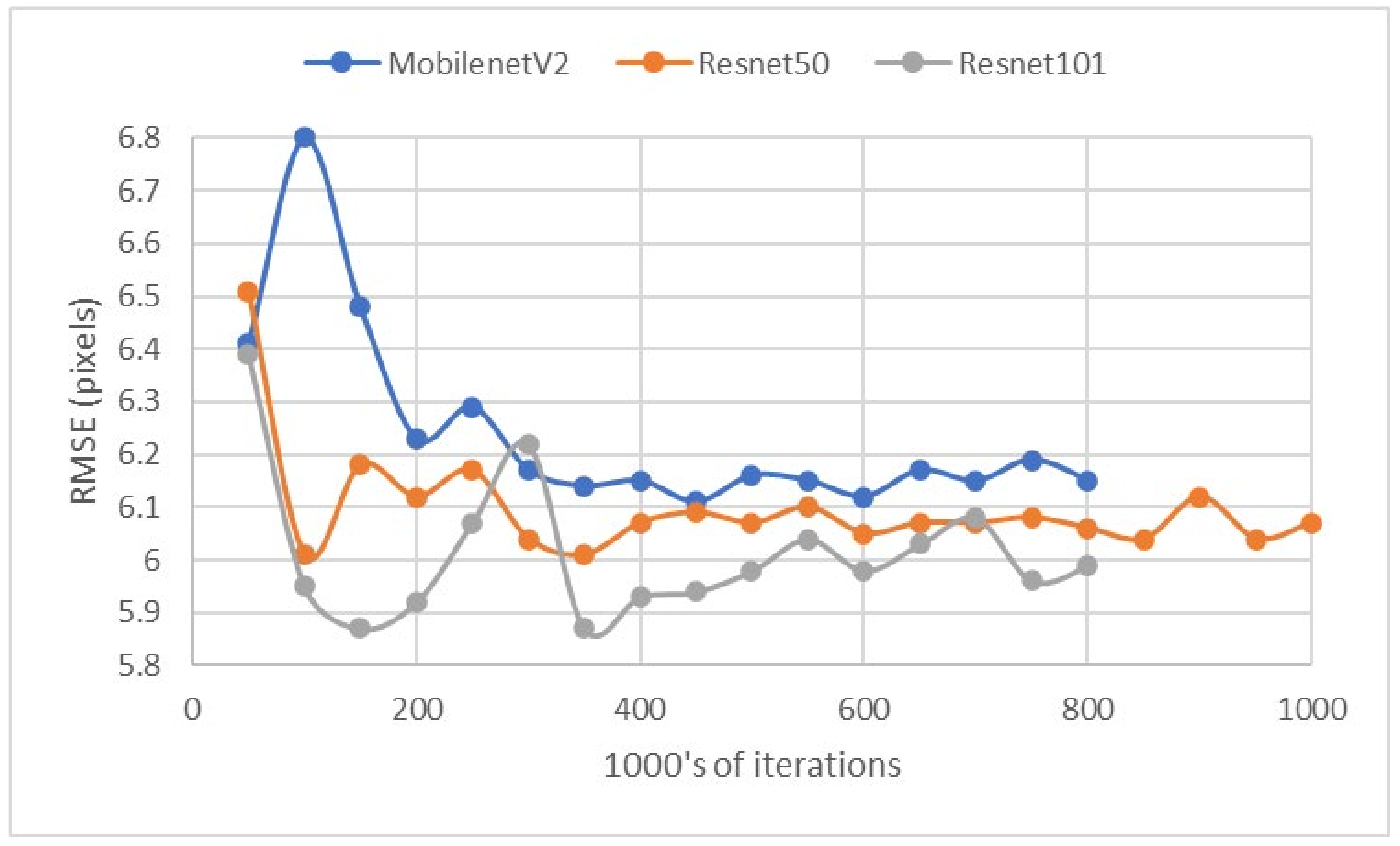
| Network | RMSE Test (p > 0.6) Pixels | Train Time 1 0.8 Million Iterations | Analyse Time 1 Frames/s |
|---|---|---|---|
| DLC (MobileNetV2_1.0) | 6.15 | 7.5 h | 190 |
| DLC (MobileNetV2_1.0) | 6.17 | 7.5 h | 190 |
| DLC (MobileNetV2_1.0) 75% | 6.28 | 7.5 h | 190 |
| DLC (MobileNetV2_1.0) 50% | 6.39 | 7.5 h | 190 |
| DLC (MobileNetV2_1.0) 25% | 6.38 | 7.5 h | 190 |
| DLC (ResNet50) | 6.07 | 16 h | 100 |
| DLC (ResNet101) | 5.99 | 30 h | 46 |
| DLC (EfficientNet b6) | 11.55 | 48 h | 14 |
| Sensor Coordinate | Pearson Correlation Coefficient |
|---|---|
| Tongue tip x | 0.37 |
| Tongue tip y | 0.88 |
| Tongue blade x | 0.39 |
| Tongue blade y | 0.93 |
| Tongue dorsum x | −0.03 |
| Tongue dorsum y | 0.44 |
| Network | RMSE Test (p > 0.6) Pixels |
|---|---|
| DLC (MobileNetV2_1.0) | 3.79 |
| DLC (ResNet50) | 3.74 |
| Lip Measure | Inter Labeller Mean/s.d./Median | DLC MobileNetV2_1.0 Mean/s.d./Median (p Value) 1 | DLC ResNet50 Mean/s.d./Median (p Value) |
|---|---|---|---|
| MSD upper lip (mm) | 0.41/0.23/0.36 | 0.59/0.29/0.54 (<0.001) | 0.59/0.40/0.47 (=0.001) |
| MSD lower lip (mm) | 0.73/0.71/0.55 | 0.86/0.75/0.64 (0.17) | 0.82/0.67/0.64 (0.65) |
| Lip aperture (mm2) | 4.6/54/6.2 | −23/61/−10 | −19/48/−11 |
| Lip width (mm) | −0.1/3.6/-0.5 | 0.8/2.4/0.7 | −0.2/3.7/0.4 |
Publisher’s Note: MDPI stays neutral with regard to jurisdictional claims in published maps and institutional affiliations. |
© 2022 by the authors. Licensee MDPI, Basel, Switzerland. This article is an open access article distributed under the terms and conditions of the Creative Commons Attribution (CC BY) license (https://creativecommons.org/licenses/by/4.0/).
Share and Cite
Wrench, A.; Balch-Tomes, J. Beyond the Edge: Markerless Pose Estimation of Speech Articulators from Ultrasound and Camera Images Using DeepLabCut. Sensors 2022, 22, 1133. https://doi.org/10.3390/s22031133
Wrench A, Balch-Tomes J. Beyond the Edge: Markerless Pose Estimation of Speech Articulators from Ultrasound and Camera Images Using DeepLabCut. Sensors. 2022; 22(3):1133. https://doi.org/10.3390/s22031133
Chicago/Turabian StyleWrench, Alan, and Jonathan Balch-Tomes. 2022. "Beyond the Edge: Markerless Pose Estimation of Speech Articulators from Ultrasound and Camera Images Using DeepLabCut" Sensors 22, no. 3: 1133. https://doi.org/10.3390/s22031133
APA StyleWrench, A., & Balch-Tomes, J. (2022). Beyond the Edge: Markerless Pose Estimation of Speech Articulators from Ultrasound and Camera Images Using DeepLabCut. Sensors, 22(3), 1133. https://doi.org/10.3390/s22031133