A Comparative Study on a Novel Quality Assessment Protocol Based on Image Analysis Methods for Color Doppler Ultrasound Diagnostic Systems

Abstract

Color Doppler (CD) imaging is widely used in diagnostics since it allows real-time detection and display of blood flow superimposed on the B-mode image. Nevertheless, to date, a shared worldwide standard on Doppler equipment testing is still lacking. In this context, the study herein proposed would give a contribution focusing on the combination of five test parameters to be included in a novel Quality Assessment (QA) protocol for CD systems testing. A first approach involving the use of the Kiviat diagram was investigated, assuming the diagram area, normalized with respect to one of the gold standards, as an index of the overall Doppler system performance. The QA parameters were obtained from the post-processing of CD data through the implementation of custom-written image analysis methods and procedures, here applied to three brand-new high-technology-level ultrasound systems. Experimental data were collected through phased and convex array probes, in two configuration settings, by means of a Doppler flow phantom set at different flow rate regimes. The outcomes confirmed that the Kiviat diagram might be a promising tool applied to quality controls of Doppler equipment, although further investigations should be performed to assess the sensitivity and specificity of the proposed approach.

1. Introduction

Ultrasound (US) is an interactive non-invasive imaging technique that provides quantitative information on anatomical districts through the propagation of ultrasound waves in soft tissues. Major US advantages compared with other imaging techniques, e.g., computed tomography or magnetic resonance, are its ease of use, real-time imaging, cost-effectiveness, portability, and patient safety [1,2]. In the last decades, active research in the US field has led to advancements in transducer technology and digital electronics with a consequent improvement of diagnostic information content [2,3]. Therefore, the US technique is applied by clinicians from different medical fields to provide diagnosis and treatment [4,5,6,7,8,9]. As a consequence, the use of US devices increased in recent years, and the worldwide market for medical ultrasound is projected to reach USD 8.4 billion in 2023, with an average annual growth rate of roughly 5.9% [10].

Color Doppler (CD) imaging, developed in the 1980s, allows the 2D real-time representation of blood flow superimposed on the anatomical image [1,2,11,12,13]. A color map codes and quantifies the velocity of blood flow inside a region of interest (or color box) adjusted by the operator on the B-mode grayscale ultrasound image as a function of the clinical requirements. Currently, CD is among the most widely used techniques in the medical field [1,2] since it is a powerful tool that allows hemodynamic monitoring and the visualization of the flow patterns in blood vessels. However, in the scientific community, controversy about whether the CD technique provides qualitative diagnostic data—non-repeatable and subjective estimations—rather than quantitative information—repeatable and objective measurements—of flow velocity still exists. This disagreement may be justified by high CD measurement uncertainties that can reach up to 50% [14]. Moreover, it is worth pointing out that a commonly accepted worldwide standard for Doppler ultrasound equipment testing has not been developed yet [15,16,17]. Attempts to define theoretical and experimental methods for medical US equipment Quality Assessment (QA) were made by several national and international organizations [16] over the years, with the consequent investigation of suitable tests for B-mode imaging, as well-documented in the literature [18,19,20,21,22,23]. Among these professional organizations, the American Institute of Ultrasound in Medicine (AIUM), the American Association of Physicists in Medicine (AAPM), the American College of Radiology (ACR), the European Federation of Societies for Ultrasound in Medicine and Biology (EFSUMB), and the Institute of Physics and Engineering (IPEM) are included.

Nowadays, although the demand for proper QA protocols has increased in the last years [16,24,25,26,27,28], performance evaluation of Doppler systems is still an open issue in the scientific research field. This is mostly due to the lack of consensus among the professional bodies about the US system configuration settings, as well as which and how many quality parameters to be processed and included in a Quality Control (QC) program for Doppler testing [16]. In this regard, the wide range of Doppler performance parameters proposed in the literature [16,25] often represents a considerable burden that requires an approach summarizing all their contributions in a few meaningful quantities that can be easily and quickly interpreted by the technician. This critical aspect is very common in several scientific fields where an effective representation of multivariate data is needed, and it is often achieved by means of a Kiviat diagram (or Kiviat plot, spider plot) [29,30]. This type of plot is characterized by a series of spokes projecting from a center point, with each spoke representing a different variable axis. The values of the variables are encompassed into the spoke length, and the plotted values are connected to form a polygon. The shape of the Kiviat diagram makes it easy to visualize and useful to compare different variables in a single graphical plot, especially when a reference or gold standard polygon is included. Nowadays, it is considered a useful comparative tool for outcome metrics since it allows both to convey a large amount of information and provide a standardized overview of different indicators [29,31]. In this regard, the Kiviat diagram could be a promising tool also in the assessment of Doppler system performance by integrating the outcomes of multiple meaningful test parameters.

Kiviat diagrams were introduced in the 1980s as a means for monitoring computer system hardware performance, and, to date, they are commonly used in several fields such as social sciences, economics, engineering, computing, and information technology and are mostly used as a tool for comparing performance metrics [29]. Although the use of the Kiviat plot in health-related literature is not so widespread, some examples should be mentioned. For instance, Kiviat plots have found utility in presenting data related to performance benchmarking at the patient and hospital levels for orthopedics surgery [31] or diagnostic performance of ultrasonography in patients with pneumonia [32].

From the above considerations, the aim of the present study is to propose and investigate the first approach to the effective combination of five parameters to be included in a novel QA protocol for Color Doppler diagnostic systems based on Kiviat diagrams. The proposed approach would give a contribution to the field since it allows quantifying the overall Doppler performance of US systems according to a probe-setting pair. Performance data could be used both to compare US systems manufactured by different companies and monitor Doppler system degradation over time. The latter usually occurs as a slow and progressive worsening of the image quality that could negatively affect the accuracy and efficacy of clinical diagnosis [33,34].

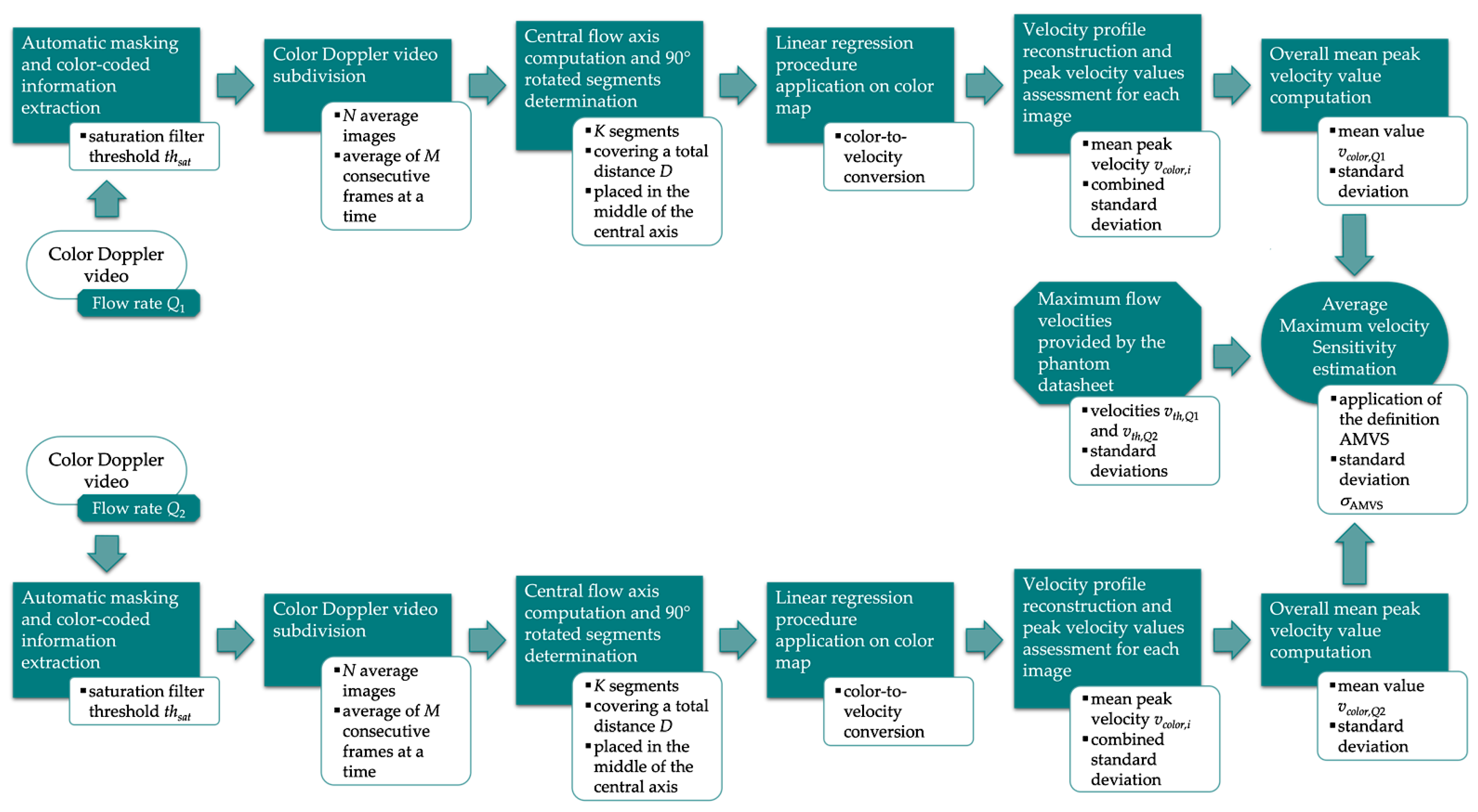
Three brand-new ultrasound systems, each of them equipped with a phased and convex array probe, were tested in two configuration settings. In this first comparative study, CD performance was evaluated in terms of: blind angle [35], registration error [36], average maximum velocity sensitivity [37], velocity measurements accuracy, and temporal resolution. These performance parameters, derived from QC tests already proposed in the literature [16] and recommended by international organizations [38,39], allow for quantifying Color Doppler functionality. They were obtained from the post-processing of Color Doppler data by means of automatic and objective image analysis procedures, whose measurement uncertainty contribution was estimated through the implementation of Monte Carlo Simulations (MCSs). One of the main advantages of the methods proposed is the possibility to overcome the intrinsic limits of visually-assessed performance tests since several test parameters recommended by the abovementioned professional organizations are qualitatively defined and suffer from operator-related errors [10,28,38,39].

The study herein proposed is organized as follows: Section 2 deals with the experimental setup adopted, the QA test parameters definition and description, as well as the normalization procedure proposed to combine and compare the outcomes retrieved. In Section 3, the measurement uncertainty analysis of the implemented image analysis-based methods through MCSs is carried out. In Section 4, experimental results are presented. In Section 5, the obtained outcomes are discussed, and future research directions are highlighted. Finally, the conclusions are outlined in Section 6.

2. Materials and Methods

2.1. Experimental Setup

The experimental setup included three high technology level US diagnostic systems, equipped with a phased (P) and a convex (C) array probe each, and a commercial Doppler flow phantom [40], whose specifications are reported in

Table 1. Doppler flow phantom: technical specifications.

Parameter	Specification
Phantom model	Doppler 403TM flow phantom
Scanning surface	patented composite film
Attenuation coefficient	0.70 ± 0.05 dB·cm−1·MHz−1
TMM (1)	patented high equivalence (HE) gelTM
TMM sound speed	1540 ± 10 m·s−1
BMF (2) sound speed	1550 ± 10 m·s−1
Flow rates	customizable, constant and pulsatile
Flow measurement range	(1.7–12.5) ± 0.4 mL·s−1
Horizontal vessel	5.0 ± 0.2 mm inner diameter at 2 cm depth
Diagonal vessel	5.0 ± 0.2 mm inner diameter at 40° from 2 to 16 cm deep

⁽¹⁾ TMM: Tissue Mimicking Material; ⁽²⁾ BMF: Blood Mimicking Fluid.

. The reference test device is constituted by a horizontal and diagonal vessel of known and constant cross-sectional area filled with blood-mimicking fluid. The flow rate can be adjusted to provide constant or pulsatile flows in the range of 1.7–12.5 mL·s⁻¹.

The two US probe models mounted on each diagnostic system were set at the best configuration settings as suggested by the product specialists (configuration A) and by reducing both pre- and post-processing settings (configuration B) to allow the comparison of the results retrieved from different US systems at similar working conditions [36,37,41,42,43]. The main settings for both configurations are listed in

Table 2. Main B-mode and Color Doppler configuration settings according to the US system.

B-Mode Setting		Configuration A			Configuration B
		System One	System Two	System Three	System One	System Two	System Three
B-mode frequency		resolution	resolution	resolution	resolution	resolution	resolution
Spatial compound imaging		ON	ON	ON	OFF	OFF	OFF
Field of view (cm)	FOV1	12	12	12	12	12	12
	FOV2	5	P: 4, C: 5	P: 4, C: 6	5	P: 4, C: 5	P: 4, C: 6
Video duration (s)		3	3	3	3	3	3
Frames resolution (px × px)		576 × 1024	920 × 1260	480 × 640	576 × 1024	920 × 1260	480 × 640
Color Doppler setting
Nominal frequency (MHz)	P	2.0	2.0	2.0	2.0	2.0	2.0
	C	2.3	2.0	2.3	2.3	2.0	2.3
Wall filter	P	medium	medium	medium	minimum	minimum	minimum
	C	medium	medium	maximum	minimum	minimum	minimum
Smoothing	P	medium	medium	minimum	minimum	minimum	minimum
	C	medium	maximum	medium	minimum	minimum	minimum
Color write priority		maximum	maximum	maximum	maximum	maximum	maximum
Line density		medium	medium	medium	low	low	low

. The three high technology level US systems, produced by different manufacturers, were anonymously addressed as system 1, system 2, and system 3. Experimental data were acquired on a portion of the diagonal vessel for the estimation of all test parameters (higher field of view setting, FOV₁), except for the blind angle. In this case, acquisitions were carried out on a portion of the horizontal vessel (lower field of view setting, FOV₂).

Color Doppler videos lasting 3 s were collected at the lowest Doppler frequency of each probe. Since the frame rate varies according to the US system and probe used, as well as to several pre- and post-processing settings (e.g., field of view, color box size, and position), a different total number of frames was acquired for each video. Therefore, a fixed number of frames n_fr was selected for the two probe models as the minimum number of frames acquired in 3 s, that in this study corresponds to n_fr = 30 and n_fr = 24 for the phased and the convex array probe, respectively. This choice allowed the comparison of the outcomes retrieved from different US systems equipped with the same probe model. In this regard, CD gain was properly set according to both the phantom flow rate and the color map scale for the assessment of all the test parameters except for the registration error. In the latter case, Color Doppler videos were acquired, increasing the CD gain control until the step before the electronic noise appeared on the US display.

Each QC parameter investigated in this study and described in the following subsection was tested at three distinct flow rate regimes (low Q_L, medium Q_M, and high Q_H) set on the Doppler phantom (

Table 3. Flow rate regimes settings according to the test parameter.

QA Test Parameter	Flow Mode	Flow Rate (mL·s−1)
		Low QL	Medium QM	High QH
Blind angle	constant	2.0	6.0	10.0
Registration error	constant	2.0	6.0	10.0
Average maximum velocity Sensitivity	constant	2.5; 4.0	7.0; 8.5	10.0; 11.5
Velocity measurements accuracy	constant	2.5	7.0	11.5
Temporal resolution	constant	–	6.0	–

). In particular, for the average maximum velocity sensitivity parameter, the flow rate was adjusted at two constant values to achieve a flow step of 1.5 mL·s⁻¹ for each regime. On the other hand, the temporal resolution parameter was tested on a single flow rate and by varying the Color Doppler line density setting (low LD_L, medium LD_M, and high LD_H).

2.2. Test Parameters for QA Protocol

2.2.1. Blind Angle

The blind angle was defined in [35] as the range of beam angles for which the US probe is not able to detect flow velocities when the insonation angle approaches 90°. In this case, the Doppler signal is almost zero, and a black flow area is displayed in the color box. From this consideration, the blind angle α was mathematically expressed as follows:

$$\alpha =2\arctan \left(\frac{a}{2h}\right)$$

(1)

where a is the blind zone transversal size, i.e., flow region in which no moving reflectors are detected, and h is the depth from the scanning surface. Such parameter was derived by considering directional accuracy at 90° performance test recommended by the AIUM [38] for Color Doppler QA. The international organization provides a qualitative definition of the test, which is performed through a visual inspection of the US system display. Conversely, the image analysis-based method, already proposed in [35], post-processes Color Doppler videos for the automatic and objective estimation of the blind angle parameter. It requires data to be collected on a portion of the Doppler phantom vessel displayed perpendicularly to the US propagation. The main steps of the measurement method, implemented by MATLAB software, are described in the following and shown in Figure 1.

Automatic masking is applied to exclude the patient information and US settings details (US image extraction), while the color-coded information is extracted through a threshold-based saturation filter th_sat [44]. Then, N average images are obtained by averaging M consecutive frames of the CD video, and a median filter with k-by-k kernel is applied to reduce color noise. After the computation of the normalized square sum of the RGB components, F parallel flow axis, placed at a fixed distance d among them, are automatically determined (Figure 2). At this point, the intensity I of each pixel intersecting the axis in the flow area at around 90° is compared with a blind threshold th_blind for the computation of the blind zone length. The blind angle is estimated for all the flow axis as defined in Equation (1), and the mean value α_i is computed together with its standard deviation σ_α,i, obtaining a first estimation of the test parameter for each average image (i = 1, …, N). Finally, the overall blind angle BA and the corresponding standard deviation σ_BA are assessed as follows:

$$\mathrm{BA}=\frac{1}{N}{\displaystyle \sum _{i=1}^N{\alpha }_i}$$

(2)

$${\sigma }_{\mathrm{BA}}=\frac{1}{N}\sqrt{{\displaystyle \sum _{i=1}^N{\sigma }_{\alpha ,i}^2}}$$

(3)

The method specifications assumed in this study are listed in

Table 4. Variables setting for blind angle parameter estimation.

Variable	Symbol	Setting
Saturation filter threshold	thsat	0.35
Number of average images	N	6
Number of averaged frames (1)	M	P: 5, C: 4
Median filter kernel	k-by-k	4-by-4 px
Number of parallel flow axis	F	3
Flow axis distance	d	1 mm
Blind threshold (2)	thblind	10

⁽¹⁾ M computed as n_fr/N; ⁽²⁾ assumed as the smallest gray level difference distinguishable from the human eye [43].

.

2.2.2. Registration Error

The Registration Error (RE) was defined in [36] as the degree of color bleeding when color write priority system control [1] is set to the maximum. It allows quantifying and monitoring the color flow misregistration, i.e., the positioning error of color flow information. The parameter was derived starting from Color/Power duplex priority control function included by the IPEM [39] among the basic functional checks for CD designed for control functioning assessment or faults detection. In this study, the semi-automatic method proposed in [36] was improved by removing the external action of the operator required to draw the vessel boundaries. The main steps of the improved method, implemented in MATLAB environment, are described in the following and shown in Figure 3.

The fully automatic method requires the processing of both a Color Doppler video and a B-mode image acquired on a Doppler flow phantom by maintaining the probe still on the scanning surface through a holder. Moreover, data need to be collected on a straight portion of the phantom vessel.

The US image extraction is applied to the grayscale anatomical image, and an adaptive threshold th_b proportional to the mean brightness V (Value in the HSV hexcone model) [45,46] of the US image is automatically determined. This threshold works as a filter for the objective detection of the lumen as well as the boundaries of the phantom vessel. The least squares method is used to determine the slope and y-intercept values of the two straight lines that best approximate the upper and lower boundaries.

On the other hand, the Color Doppler video is processed both through the US image extraction and a threshold-based saturation filter th_sat [44] to extract the color-coded information. Then, N average images are obtained by averaging M consecutive frames, and the normalized square sum of the RGB components is computed. As in [36], the two abovementioned straight lines are used to subdivide and crop the color box of each average image into two different sub-boxes (Figure 4). At this point, the intensity I of each pixel in the sub-boxes is compared with the threshold th_blind for the computation of n_out, i.e., the number of colored pixels outside the vessel walls. The percentage registration error for each average image RE_%,i (i = 1, …, N) is estimated by applying the following mathematical expression [36]:

$${\mathrm{RE}}_{\%,i}=\frac{n_{out,i}}{n_{box,i}}\cdot 100$$

(4)

where n_box,i is the number of pixels in the entire color box of the i-th image whose intensity is above the threshold.

Finally, the overall percentage registration error RE_% is computed as the mean value of the N percentage registration values retrieved, and the standard deviation σ_RE% is estimated. According to Equation (4), the test parameter is expected to be 0%, i.e., no color flow misregistration.

The method specifications assumed in this study are listed in

Table 5. Variables setting for registration error parameter estimation.

Variable	Symbol	Setting
Brightness filter threshold	thb	μb(1)
Saturation filter threshold	thsat	0.35
Number of average images	N	6
Number of averaged frames (2)	M	P: 5, C: 4
Blind threshold (3)	thblind	10

⁽¹⁾ μ_b varies proportionally to the mean brightness V of the image; ⁽²⁾ M computed as n_fr/N; ⁽³⁾ assumed as the smallest gray level difference distinguishable from the human eye [43].

.

2.2.3. Average Maximum Velocity Sensitivity

The Average Maximum Velocity Sensitivity (AMVS) is a sensitivity test parameter defined and preliminarily investigated in [41] for Pulsed Wave Doppler QC and in [37] for Color Doppler QC. It allows quantifying the US system response to flow variations provided by a reference device. In this study, the method already proposed in [37] was improved in order to process the Color Doppler videos. The main steps of the updated method, implemented through a custom-written algorithm in MATLAB, are described in the following and shown in Figure 5.

As already described for the previous parameters, the US image extraction is carried out, while the color-coded information is extracted through the threshold-based saturation filter th_sat [44]. Then, N average images are obtained by averaging M consecutive frames of the Color Doppler video. At this point, the central flow axis is determined to automatically draw K segments rotated at 90° covering a total distance D and placed in the middle zone of the axis (Figure 6). The linear regression procedure proposed in [44] is applied for color-to-velocity conversion, allowing the reconstruction of the velocity profile associated with each segment (Figure 7). The peak velocity of each profile is assessed, and consequently, the mean peak velocity value v_color,i (i = 1, …, N) is computed together with the standard deviation. The latter is combined with the uncertainty contribution related to the linear regression procedure [44]. These computations are repeated for all the N average images, obtaining an overall mean peak velocity value v_color and the corresponding standard deviation retrieved through the uncertainty propagation law. All the processing steps described above are repeated for two different constant flow rate regimes (Q₁ and Q₂) set on the flow phantom, therefore determining v_color,Q1 and v_color,Q2. Finally, AMVS parameter is assessed as follows:

$$\mathrm{AMVS}=\frac{\Delta v_{color}}{\Delta v_{th}}$$

(5)

where Δv_color is the difference between v_color,Q1 and v_color,Q2, while Δv_th is the difference between the corresponding theoretical maximum flow velocities (v_th,Q1 and v_th,Q2) provided by the phantom. On the other hand, AMVS standard deviation σ_AMVS is estimated through the uncertainty propagation law as follows:

$${\sigma }_{\mathrm{AMVS}}=\mathrm{AMVS}\sqrt{{\left(\frac{{\sigma }_{\Delta vcolor}}{\Delta v_{color}}\right)}^2+{\left(\frac{{\sigma }_{\Delta vth}}{\Delta v_{th}}\right)}^2}$$

(6)

where the two contributions in the square sum are the relative standard deviations of Δv_color and Δv_th. According to Equation (5), the dimensionless parameter is expected to be 1, i.e., maximum system sensitivity.

The method specifications assumed in this study are listed in

Table 6. Variables setting for both AMVS and VeMeA parameters estimation.

Variable	Symbol	Setting
Saturation filter threshold	thsat	0.35
Number of average images	N	6
Number of averaged frames (1)	M	P: 5, C: 4
Number of rotated segments	K	16
Covered central axis portion	D	20 mm

⁽¹⁾ M computed as n_fr/N.

.

2.2.4. Velocity Measurements Accuracy

Velocity Measurements Accuracy (VeMeA) was derived from a QC test already proposed in literature [16], i.e., the mean velocity estimation, which provides an assessment of the system accuracy in the mean scatterer velocity estimation. In this study, a novel image analysis method is proposed and investigated for the automatic estimation of the test parameter through the post-processing of Color Doppler videos. The main steps of the method, implemented through an ad hoc algorithm in MATLAB, are described in the following and shown in Figure 8.

The post-processing steps of the novel method are based on the previous one for AMVS parameter assessment. In fact, the following operations are replicated: automatic masking (US image extraction), threshold-based saturation filtering th_sat, averaging of M consecutive frames to obtain N average images, computation of the central flow axis as well as K segments rotated at 90° covering a total distance D and placed in the middle zone of the axis (Figure 6). Then, the linear regression procedure [44] is applied for color-to-velocity conversion of the color map, allowing the reconstruction of the velocity profile associated with each segment (Figure 7). At this point, the average velocity of each profile is assessed and, consequently, the mean velocity value ${\overline{v}}_{color,i}$ (i = 1, …, N) is computed together with the standard deviation, which, in turn, is combined with the uncertainty contribution related to the linear regression procedure [44]. These computations are repeated for all the N average images, obtaining an overall mean velocity value ${\overline{v}}_{color}$ and the corresponding standard deviation ${\sigma }_{\overline{v}color}$. Finally, VeMeA parameter is estimated as follows:

$$\mathrm{VeMeA}=\frac{\left|{\overline{v}}_{color}-{\overline{v}}_{th}\right|}{{\overline{v}}_{th}}$$

(7)

where ${\overline{v}}_{th}$ is the corresponding theoretical average flow velocity provided by the Doppler phantom. As regards the standard deviation of the parameter (σ_VeMeA), it is estimated by applying the uncertainty propagation law as follows:

$${\sigma }_{\mathrm{VeMeA}}=\mathrm{VeMeA}\sqrt{{\left(\frac{{\sigma }_{\overline{v}color}}{{\overline{v}}_{color}}\right)}^2+{\left(\frac{{\sigma }_{\overline{v}th}}{{\overline{v}}_{th}}\right)}^2}$$

(8)

where ${\sigma }_{\overline{v}th}$ is the flow velocity standard deviation derived from the phantom datasheet. According to the definition proposed, VeMeA is a dimensionless parameter that is expected to be as close as possible to 0, i.e., high system accuracy.

The method specifications assumed in this study are listed in Table 6.

2.2.5. Temporal Resolution

Temporal Resolution (TR) is the minimum temporal interval for which two distinct events can be identified. Since flow changes can occur very rapidly, TR was included among the recommended QC measurements [16]. In this study, a novel image analysis method is proposed and investigated as a first attempt for the automatic estimation of CD temporal resolution related to the US system settings. The main steps of the method, developed in MATLAB environment, are described in the following and shown in Figure 9.

The method requires the processing of a Color Doppler and a B-mode image collected on a Doppler flow phantom by maintaining the probe still and the US setting constant.

Firstly, automatic masking is applied both to the grayscale and Color image to extract the diagnostic and color box, respectively, allowing the computation of the total diagnostic area A_tot as well as the color box area A_color. In particular, A_color is retrieved by paying attention not to include the pixels belonging to the box perimeter. Then, the temporal resolution parameter is estimated by applying the following mathematical expression:

$$TR=\frac{F{R}_{duplex}}{F{R}_{Bmode}}\cdot \frac{A_{color}}{A_{tot}}$$

(9)

where FR_duplex is the frame rate of the duplex imaging (CD imaging superimposed on the B-mode one), while FR_Bmode is the frame rate of the grayscale image only. According to the definition, when the color box is adjusted so as to include all the diagnostic box area (A_color/A_tot = 1), the ratio FR_duplex/FR_Bmode is expected to reach a maximum of 0.5. This assumption is based on the hypothesis that, under maximum system performance conditions, the frame rate of the duplex system may be half that of the B-mode imaging due to the computational cost of the Doppler processing.

2.3. Data Normalization

Normalization is an essential step in data analysis. Since the optimal value was different for each proposed test parameter (

Table 7. Summary of the optimal values for each proposed test parameter.

QA Test Parameter	Acronym	Optimal Value
Blind angle	BA	0°
Percentage registration error	RE%	0%
Average maximum velocity sensitivity	AMVS	1
Velocity measurements accuracy	VeMeA	0
Temporal resolution	TR	0.5

), a normalization procedure to extract comparable values for all QA parameters was considered.

Specifically, normalized values were expected to be in the range [0, 1], while the gold standard was 1 for all parameters. Normalized values for blind angle, registration error, average maximum velocity sensitivity, velocity measurements accuracy and temporal resolution were computed as follows:

$$B{A}^{\ast }=1-\frac{BA}{B{A}_{\lim }}$$

(10)

$$R{E}^{\ast }=1-\frac{RE}{100}$$

(11)

$${\mathrm{AMVS}}^{*}=1-\left(\left|\mathrm{AMVS}-1\right|\right)$$

(12)

$${\mathrm{VeMeA}}^{*}=1-\mathrm{VeMeA}$$

(13)

$$T{R}^{\ast }=\sqrt{\frac{TR}{T{R}_{opt}}}$$

(14)

where the symbol (*) denotes the normalized value for each test parameter. In particular, BA_lim in Equation (10) is the maximum expected BA value that in this study was assumed equal to 45°, while TR_opt in Equation (14) indicates the optimal value of TR. The square root in the TR normalization was chosen in order to increase the dynamic of this parameter and appreciate small differences among TR results.

3. Monte Carlo Simulation

The measurement uncertainty contribution due to the image analysis-based methods was estimated through the Monte Carlo Simulation [47], a proper and robust tool already experienced in previous studies [43,48,49]. An MCS with 10⁴ iterations was run for each combination of test parameters, US systems, and probes, as well as configuration and phantom settings. The standard deviation (SD) from each MCS was then estimated and combined with the corresponding repeatability SD retrieved in Section 2.2.

Uniform distributions, expressed as mean ± SD, were assigned to the variables influencing the assessment of the QC parameters investigated in this study (

Table 8. Distribution setting in MCSs for measurement uncertainty estimation of the image analysis method for QC test parameters assessment.

Blind Angle Assessment	Symbol	Distribution	Mean ± SD
Saturation filter threshold	thsat ± σsat	uniform	0.35 ± 0.01
Median filter kernel	k ± σk	uniform	4 ± 1 px
Flow axis distance	d ± σd	uniform	1.0 ± 0.3 mm
Blind threshold	thblind ± σblind	uniform	10 ± 1
Registration error assessment
Brightness filter threshold	thb ± σb	uniform	μb ± 0.06μb
Saturation filter threshold	thsat ± σsat	uniform	0.35 ± 0.01
Blind threshold	thblind ± σblind	uniform	10 ± 1
AMVS and VeMeA assessment
Saturation filter threshold	thsat ± σsat	uniform	0.35 ± 0.01
Covered central axis portion	D ± σD	uniform	20 ± 1 mm
First segment position on the axis	x ± σx	uniform	x0 ± 1 mm (1)
Temporal resolution assessment
Duplex imaging frame rate	FRduplex ± σduplex	uniform	FRduplex ± 1
B-mode imaging frame rate	FRBmode ± σBmode	uniform	FRBmode ± 1
Color box area	Acolor ± σcolor	uniform	Acolor ± 0.03Acolor
Total diagnostic area	Atot ± σtot	uniform	Atot ± 0.03Atot

⁽¹⁾ x₀ is the generic position of the first segment on the central flow axis.

). In the MCSs involving Color Doppler video processing, both the number of average images N and the number of averaged frames M were maintained constant throughout the iterations, while the frames to be averaged were randomized at each cycle without repetition among all the frames acquired in 3 s.

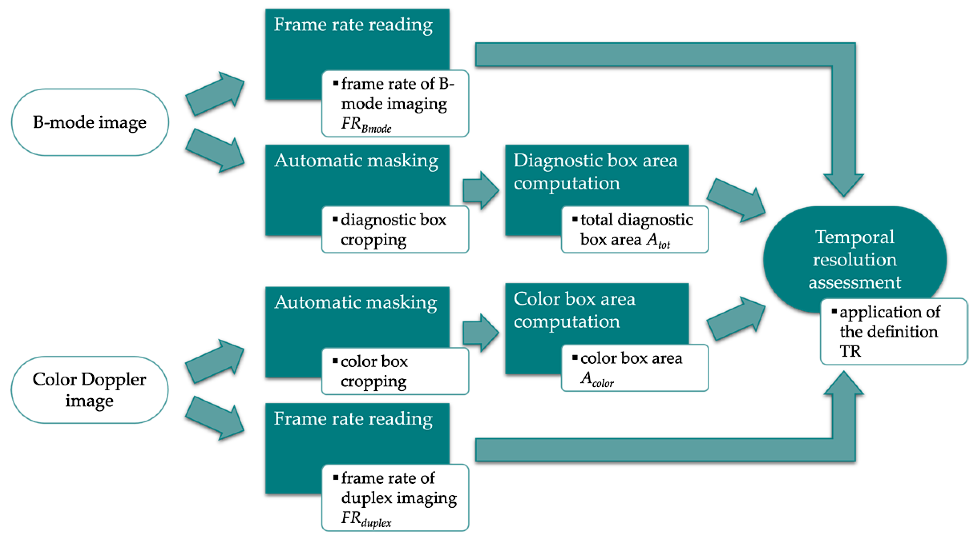
The distributions for the blind angle assessment were assigned in an analogous way to [35], while those for the registration error assessment also included an input distribution associated with the brightness filter threshold whose standard deviation σ_b was set to 6% of the mean value μ_b. On the other hand, the same distributions were used for the assessment of both AMVS and VeMeA parameters. Finally, for temporal resolution parameter assessment, uniform distributions were assigned to the quantities in Equation (9), assuming for both A_color and A_tot a standard deviation set to 3% of the corresponding mean value.

4. Results

Experimental outcomes for each combination of test parameters, US systems, and probes, as well as configuration and phantom settings, are reported as mean ± SD in

Table 9. Blind angle parameter results (mean ± SD).

Probe Model	Flow Rate Regime	Configuration A			Configuration B
		System One	System Two	System Three	System One	System Two	System Three
Phased array	QL	15.7° ± 2.1°	17.9° ± 1.6°	6.9° ± 2.1°	15.4° ± 2.3°	19.2° ± 2.0°	11.1° ± 2.6°
	QM	9.8° ± 2.5°	21.6° ± 1.6°	12.8° ± 2.4°	12.0° ± 2.5°	18.1° ± 2.1°	13.3° ± 2.5°
	QH	2.0° ± 1.1°	2.0° ± 1.2°	5.6° ± 1.2°	0.5° ± 0.4°	7.7° ± 2.4°	7.4° ± 2.6°
Convex array	QL	36° ± 3°	30° ± 5°	30° ± 6°	20° ± 3°	11° ± 3°	10° ± 4°
	QM	16.1° ± 2.7°	36.8° ± 2.6°	25° ± 6°	13.1° ± 2.1°	6.2° ± 2.6°	17° ± 5°
	QH	5.6° ± 1.2°	9.6° ± 2.8°	27° ± 5°	4.1° ± 1.3°	2.0° ± 1.3°	28° ± 5°

,

Table 10. Percentage registration error parameter results (mean ± SD).

Probe Model	Flow Rate Regime	Configuration A			Configuration B
		System One	System Two	System Three	System One	System Two	System Three
Phased array	QL	(3.2 ± 1.9)%	(3.3 ± 1.2)%	(12 ± 8)%	(6.2 ± 2.1)%	(12.0 ± 2.8)%	(7.9 ± 2.3)%
	QM	(9.4 ± 2.9)%	(25 ± 14)%	(13 ± 6)%	(15 ± 3)%	(33 ± 12)%	(28 ± 7)%
	QH	(20 ± 5)%	(34 ± 6)%	(27 ± 3)%	(18 ± 5)%	(55.1 ± 3.2)%	(48 ± 4)%
Convex array	QL	(25.2 ± 2.2)%	(15.3 ± 0.4)%	(4.8 ± 1.4)%	(22.3 ± 1.4)%	(12.6 ± 0.9)%	(15.0 ± 2.8)%
	QM	(36 ± 5)%	(32 ± 6)%	(3.2 ± 1.4)%	(20 ± 3)%	(32 ± 7)%	(25 ± 7)%
	QH	(34.3 ± 1.7)%	(20 ± 3)%	(23 ± 3)%	(36.4 ± 1.8)%	(16 ± 3)%	(30 ± 7)%

,

Table 11. Average Maximum Velocity Sensitivity parameter results (mean ± SD).

Probe Model	Flow Rate Regime	Configuration A			Configuration B
		System One	System Two	System Three	System One	System Two	System Three
Phased array	QL	0.44 ± 0.12	0.55 ± 0.15	0.44 ± 0.12	0.41 ± 0.11	0.55 ± 0.15	0.58 ± 0.15
	QM	0.51 ± 0.21	0.59 ± 0.42	0.29 ± 0.16	0.53 ± 0.21	0.43 ± 0.36	0.39 ± 0.18
	QH	0.50 ± 0.26	0.07 ± 0.20	0.39 ± 0.25	0.48 ± 0.25	0.03 ± 0.14	0.68 ± 0.40
Convex array	QL	0.54 ± 0.14	0.62 ± 0.16	0.48 ± 0.12	0.45 ± 0.12	0.60 ± 0.15	0.46 ± 0.12
	QM	0.36 ± 0.18	0.39 ± 0.17	0.45 ± 0.17	0.30 ± 0.17	0.48 ± 0.19	0.48 ± 0.18
	QH	0.33 ± 0.22	0.57 ± 0.27	0.55 ± 0.27	0.33 ± 0.25	0.43 ± 0.31	0.54 ± 0.45

,

Table 12. Velocity Measurements Accuracy parameter results (mean ± SD).

Probe Model	Flow Rate Regime	Configuration A			Configuration B
		System One	System Two	System Three	System One	System Two	System Three
Phased array	QL	0.38 ± 0.07	0.18 ± 0.12	0.38 ± 0.08	0.44 ± 0.06	0.20 ± 0.12	0.17 ± 0.09
	QM	0.50 ± 0.04	0.12 ± 0.07	0.34 ± 0.04	0.49 ± 0.04	0.25 ± 0.07	0.33 ± 0.04
	QH	0.42 ± 0.03	0.14 ± 0.05	0.43 ± 0.04	0.47 ± 0.03	0.32 ± 0.07	0.49 ± 0.04
Convex array	QL	0.24 ± 0.08	0.05 ± 0.11	0.20 ± 0.08	0.17 ± 0.08	0.09 ± 0.11	0.20 ± 0.08
	QM	0.30 ± 0.04	0.19 ± 0.05	0.25 ± 0.04	0.30 ± 0.04	0.17 ± 0.06	0.29 ± 0.04
	QH	0.39 ± 0.03	0.42 ± 0.04	0.51 ± 0.05	0.33 ± 0.04	0.40 ± 0.04	0.64 ± 0.03

and

Table 13. Temporal resolution parameter results (mean ± SD).

Probe Model	CD Line Density	Configuration A			Configuration B
		System One	System Two	System Three	System One	System Two	System Three
Phased array	LDL	0.10 ± 0.01	0.10 ± 0.01	0.07 ± 0.01	0.17 ± 0.01	0.12 ± 0.01	0.08 ± 0.01
	LDM	0.08 ± 0.01	0.09 ± 0.01	0.06 ± 0.01	0.14 ± 0.01	0.10 ± 0.01	0.06 ± 0.01
	LDH	0.06 ± 0.01	0.08 ± 0.01	0.05 ± 0.01	0.11 ± 0.01	0.09 ± 0.01	0.06 ± 0.01
Convex array	LDL	0.10 ± 0.01	0.18 ± 0.02	0.17 ± 0.01	0.14 ± 0.02	0.21 ± 0.02	0.19 ± 0.01
	LDM	0.09 ± 0.01	0.14 ± 0.02	0.13 ± 0.01	0.12 ± 0.02	0.16 ± 0.02	0.15 ± 0.01
	LDH	0.07 ± 0.01	0.12 ± 0.02	0.11 ± 0.01	0.10 ± 0.02	0.14 ± 0.02	0.12 ± 0.01

. Standard deviations were computed by combining σ_BA, σ_RE%, σ_AMVS and σ_VeMeA values with the corresponding ones estimated from MCSs. As regards the TR parameter, standard deviations were retrieved directly from the data distributions.

From blind angle outcomes (Table 9), it can be noticed that the tested phased probes showed global compatibility between the two configuration settings by considering the same flow regime. Such compatibility was no longer guaranteed for the convex array probes, for which higher BA results were retrieved in configuration A than in B. Moreover, the results obtained for both the probes of system one showed, as expected, a decreasing trend for increasing flow rates, while a reversed trend was found for the convex array probe of system three in configuration B. As per system two in configuration A, the mean value retrieved at medium flow regime Q_M was higher than the one at high flow regime Q_H for both the probes, and the same behavior was also found for the phased array probe of system three. Finally, for the convex probe of system three in configuration A, blind angle results were compatible and did not show a specific trend.

As regards the percentage registration error, the outcomes obtained (Table 10) for the phased array probes globally showed an increasing trend for increasing flow rates, while a well-defined behavior cannot be inferred for the convex array probes. Furthermore, RE_% results for system one were the closest to 0% among all three phased probe-system pairs in both configurations. On the other hand, system three, equipped with the convex array probe, showed results closer to the optimal value in configuration A only, probably due to the higher wall filter setting (Table 2) included in its clinical preset.

AMVS outcomes (Table 11) were retrieved among velocities belonging to the same flow regime, maintaining a fixed flow step of 1.5 mL·s⁻¹, as listed in Table 3. They show a similar behavior between the two configurations independently of the US system for both probe models. The lowest sensitivity values that significantly deviate from one were obtained with the phased array probe of system two at a high flow rate regime Q_H.

By focusing on VeMeA outcomes (Table 12), an increasing trend for increasing flow rates was found for all the convex array probes, while a distinct behavior cannot be inferred for the phased array ones. They were generally compatible between configurations A and B, and for system one was noticed that the results obtained for the convex probe were always lower than the corresponding ones for the phased probe. On the other hand, independently of the probe model, system two showed a higher occurrence of results closest to the optimal value.

Finally, temporal resolution results (Table 13) obtained for both probe models of all US systems showed, as expected, a decreasing trend for increasing Color Doppler line density setting. Moreover, by comparing each outcome in configuration A with the corresponding one in configuration B, higher TR values were always found in the latter configuration. This could probably be due to the reduction of both pre- and post-processing settings. Best outcomes (closest to 0.5) were found for system one and system two with the phased and convex array probes, respectively.

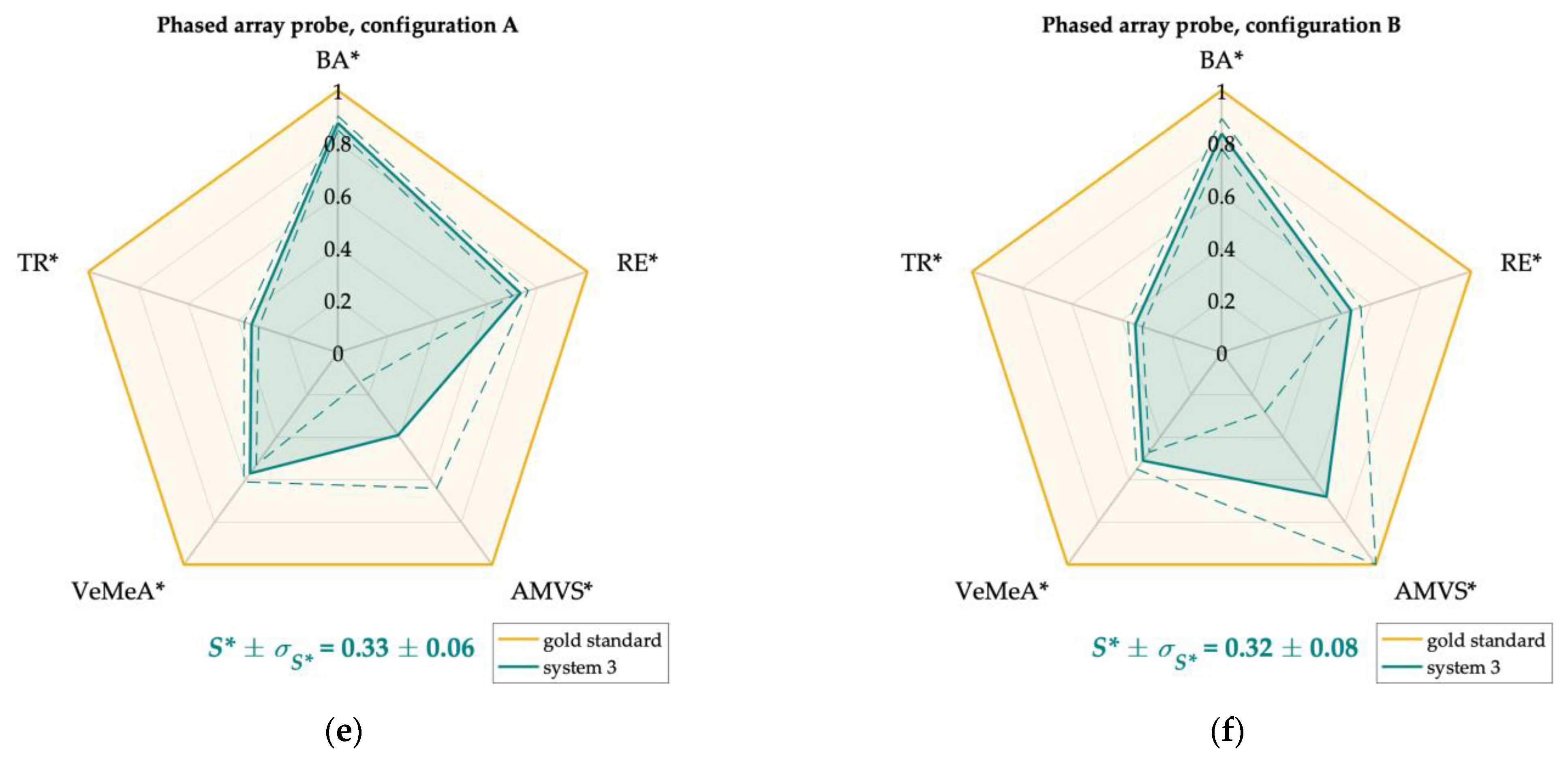
Experimental results were normalized according to the normalization steps described in Section 2.3 to allow the combination of the five test parameters retrieved for each probe at the same phantom and system settings. This allowed their representation on Kiviat diagrams and the direct comparison with the gold standard for which all the normalized QA test parameters were set to one. Therefore, the area of each polygon was computed and used as an index to quantify the overall Doppler performance of the US systems depending on the probe-configuration pair: the greater the polygon area, the higher the Doppler system performance. For ease of interpretation, the areas of the diagrams were normalized with respect to the total area of the gold standard. In this perspective, the normalized area was expected to be as close as possible to one.

Kiviat diagrams for systems one, two, and three equipped with phased and convex array probes in configurations A and B are shown in Figure 10 and Figure 11. In particular, the QA parameters retrieved at a high flow rate Q_H (

Table 14. Normalized QA test parameters and Kiviat diagram areas (mean ± SD) for systems 1, 2 and 3 equipped with phased array probes in configurations A and B at high flow regime.

US System	Configuration	BA*	RE*	AMVS*	VeMeA*	TR*	S* ± σS*
1	A	0.96 ± 0.02	0.80 ± 0.05	0.50 ± 0.26	0.58 ± 0.03	0.40 ± 0.02	0.41 ± 0.07
	B	0.99 ± 0.01	0.82 ± 0.05	0.48 ± 0.25	0.53 ± 0.03	0.53 ± 0.02	0.45 ± 0.07
2	A	0.95 ± 0.03	0.66 ± 0.06	0.07 ± 0.20	0.86 ± 0.05	0.42 ± 0.02	0.33 ± 0.04
	B	0.83 ± 0.05	0.45 ± 0.03	0.03 ± 0.14	0.68 ± 0.07	0.45 ± 0.02	0.23 ± 0.03
3	A	0.86 ± 0.03	0.73 ± 0.03	0.39 ± 0.25	0.57 ± 0.04	0.35 ± 0.03	0.33 ± 0.06
	B	0.84 ± 0.06	0.52 ± 0.04	0.68 ± 0.40	0.51 ± 0.04	0.35 ± 0.03	0.32 ± 0.08

) were used for the diagrams plot of the phased array probes since this model, preferred for echocardiography, is designed to detect high blood velocities [1]. On the other hand, the QA parameters at medium flow rate Q_M (

Table 15. Normalized QA test parameters and Kiviat diagram areas (mean ± SD) for systems 1, 2 and 3 equipped with convex array probes in configurations A and B at medium flow regime.

US System	Configuration	BA*	RE*	AMVS*	VeMeA*	TR*	S* ± σS*
1	A	0.64 ± 0.06	0.64 ± 0.05	0.36 ± 0.18	0.70 ± 0.04	0.42 ± 0.02	0.29 ± 0.05
	B	0.71 ± 0.05	0.80 ± 0.03	0.30 ± 0.17	0.70 ± 0.04	0.49 ± 0.04	0.34 ± 0.05
2	A	0.18 ± 0.06	0.68 ± 0.06	0.39 ± 0.17	0.81 ± 0.05	0.53 ± 0.04	0.25 ± 0.05
	B	0.86 ± 0.06	0.68 ± 0.07	0.48 ± 0.19	0.83 ± 0.06	0.56 ± 0.04	0.45 ± 0.06
3	A	0.44 ± 0.14	0.97 ± 0.01	0.45 ± 0.17	0.75 ± 0.04	0.51 ± 0.02	0.36 ± 0.07
	B	0.62 ± 0.11	0.75 ± 0.07	0.48 ± 0.18	0.71 ± 0.04	0.55 ± 0.02	0.38 ± 0.06

) were used for the diagrams plot of the convex array probes since this model is typically designed for abdominal imaging [1]. As regards the TR parameter, results obtained at medium CD line density setting LD_M were considered for both probe models. Alongside the Kiviat diagram plot, the normalized mean area S* and the corresponding standard deviation σ_S* were computed (Figure 10 and Figure 11). The latter was estimated through the error propagation law.

Finally, as regards the normalized areas (Table 14 and Table 15), compatible performance was found between the two configurations for both probe models of systems one and three. As regards system two, a higher area was obtained in configurations A and B for the phased and convex array probes, respectively. By focusing on the phased array probes, system one showed the highest diagram area independently of the configuration setting (0.41 ± 0.07 and 0.45 ± 0.07 in A and B, respectively), while the lowest one was found for system two in configuration B (0.23 ± 0.03). On the other hand, the highest and lowest areas for the convex array probes were found for system two in configuration B (0.45 ± 0.06) and A (0.25 ± 0.05), respectively.

5. Discussion

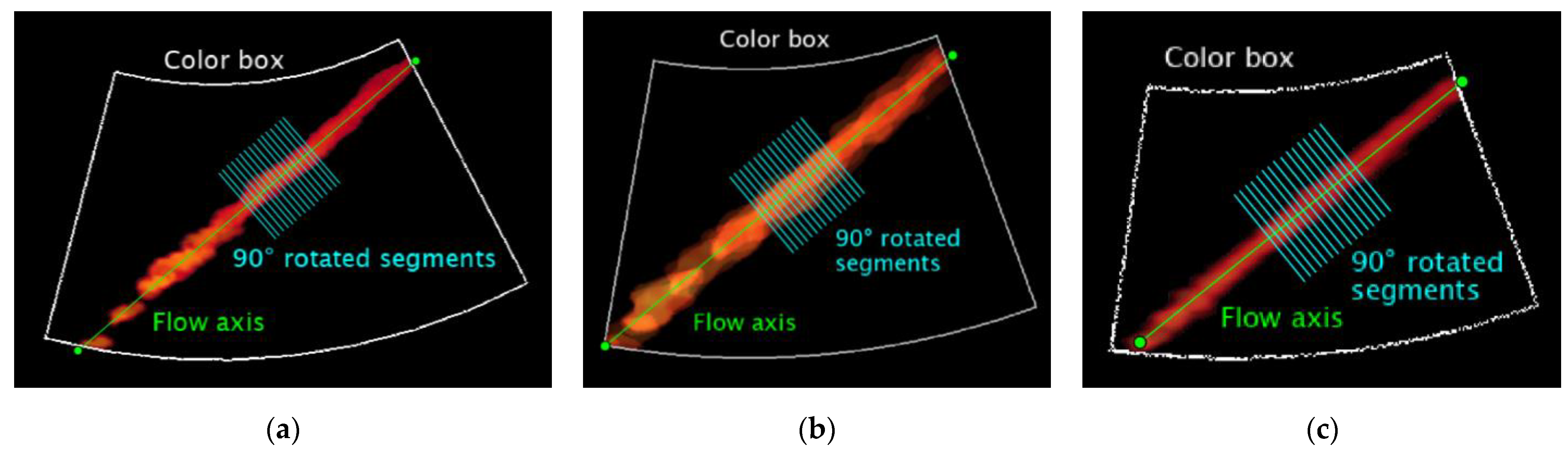
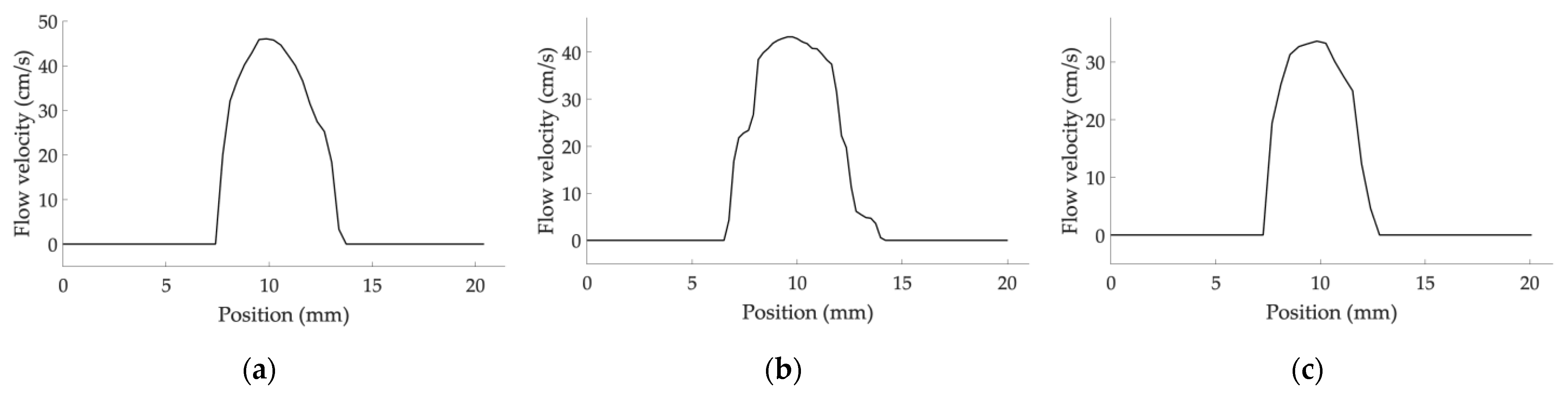
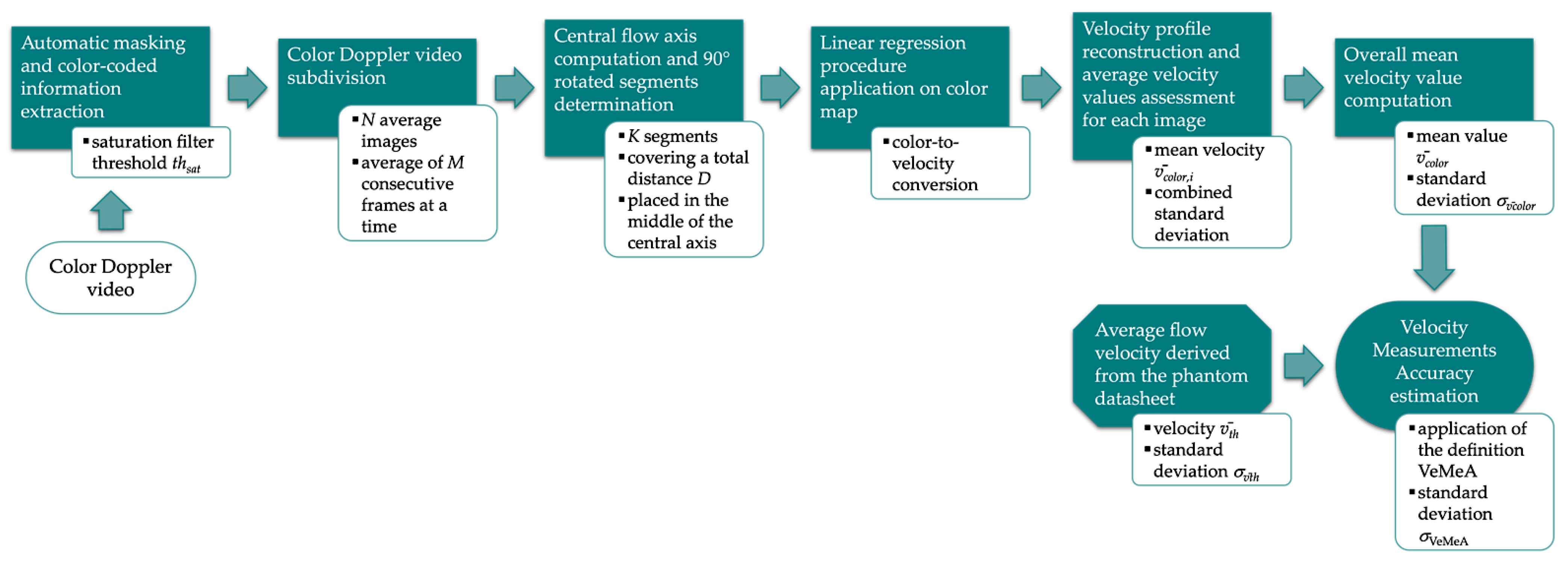
The present study is proposed as a first approach to the combination of five Doppler test parameters based on the Kiviat diagram to quantify the performance of the US systems according to a probe-setting pair. As a first attempt, the diagram area normalized with respect to the gold standard was assumed as an index of the overall Color Doppler system performance. The assessed parameters were the blind angle, registration error, average maximum velocity sensitivity, velocity measurements accuracy, and temporal resolution. They were objectively assessed through custom-written image analysis-based methods and procedures (Figure 1, Figure 3, Figure 5, Figure 8 and Figure 9) and then normalized in the same range for the graphical representation. Three brand-new ultrasound systems, equipped with a phased and convex array probe each, were tested in two configuration settings at different flow rate regimes set on a Doppler reference device (Table 2 and Table 3).

As regards the results obtained for each single test parameter (Table 9, Table 10, Table 11, Table 12 and Table 13), it should be noticed that independently of the US system tested, BA outcomes retrieved for the phased array probes were the closest to the optimal value. By comparing the US systems, better results (closest to 0) were found for both probe models of system one independently of the configuration setting. By focusing on the percentage registration error, the phased array probes globally showed better results (closest to 0) with respect to the convex array one for both systems one and two in configuration A. Moreover, independently of the configuration, RE_% results for system one were the closest to the optimal value among all three phased probe-system pairs. On the other hand, AMVS results obtained for the probes of the three US systems are globally compatible among them at both configurations. However, it should also be noted that the sensitivity index is the one showing the highest SD values among the proposed QA test parameters. By considering the VeMeA parameter, the results were generally compatible between the two configurations and independent of the probe model. Lastly, temporal resolution results for both probe models of all US systems always showed, as expected, higher TR values in configuration B, probably due to the reduction of pre- and post-processing settings. Best outcomes (closest to 0.5) were found for system one and system two with the phased and convex array probes, respectively. Moreover, SD values were almost constant for all the tested phased probes in both configurations, while a limited increment was found for some convex probes.

The use of Kiviat diagrams allowed combining the quality parameters (Figure 10 and Figure 11) and estimating a single index (normalized diagram area) that provided a more immediate assessment of the CD system quality. QA parameters assessed at high and medium flow rates were used for the diagrams plot of the phased and the convex array probes, respectively. Conversely, temporal resolution results at a medium number of CD scan lines were considered for both probe models. For these cases, the outcomes (Table 14 and Table 15) confirmed that a higher polygon area was found for the probe-system pair showing higher values of the test parameters discussed above (e.g., phased array probe of system one in both configurations). Moreover, diagrams with comparable areas corresponded to US systems whose test parameters showed compatibility. These aspects suggest that the Kiviat diagram may be a useful tool for US system assessment since it seems to be directly related to the system performance. Globally, the normalized areas did not show, as expected, significant discrepancies among them since the US systems tested in this study were all brand-new systems at the same technology level. As a last remark, it should be noted that the normalized area of the diagram, together with its shape, has the advantage of preserving the relationship among the test parameters with respect to other mathematical operators, such as the arithmetic or geometric mean of the test parameters. Moreover, the Kiviat plot could provide the technician with a quick overview of the values of the single parameters highlighting both weaknesses and strengths of the Doppler system under testing and allowing the US system performance monitoring over time.

Despite the promising results, the present study is a first attempt at the use of the Kiviat diagram applied to QCs of Doppler equipment. Therefore, further investigations should be performed to assess the sensitivity as well as determine the specificity of the proposed approach. In particular, studies aimed to estimate how much the variation (due to the US system deterioration) of one (or more) of the quality parameters affects the diagram area are going to be carried out. On the other hand, US systems that have been used in the clinical setting for a few years should be tested, and the areas of their Kiviat diagrams should be compared with the ones retrieved for brand-new systems at the same technology level. This could be useful to understand whether the proposed approach is able to detect significant discrepancies among the areas of the diagrams due to an objectively evident state of deterioration. As a last remark, further investigations may include the deepening of the relationship among the QA parameters and how it could affect the shape of the Kiviat diagram.

6. Conclusions

Quality assessment is necessary in the US field, as for any other medical imaging equipment, in order to maintain image quality in accordance with the manufacturer’s recommendations, ensure both patient and operator safety, and comply with regulatory and accreditation requirements. Since Color Doppler is among the most used and widespread Doppler techniques in diagnostic imaging, the need for an internationally accepted quality standard for Doppler equipment is deemed important. In this regard, the study herein proposed would give a contribution to this field by investigating a first approach involving the use of the Kiviat diagram applied to QCs of Doppler equipment. Five QA parameters were objectively assessed through the post-processing of CD data, and after a normalization process, they were combined together to be represented within a single plot and summarized in a representative index. On the basis of the promising outcomes obtained and their limitations, further studies are going to be carried out for a thorough characterization of the proposed approach, including a higher number of US diagnostic systems and probe models (e.g., linear array probes).

References

1. Hoskins, P.R.; Martin, K.; Thrush, A. Diagnostic Ultrasound. Physics and Equipment, 3rd ed.; CRC Press: Boca Raton, FL, USA, 2019. [Google Scholar]
2. Wang, Y.; Chai, H.; Ye, R.; Li, J.; Liu, J.B.; Lin, C.; Peng, C. Point-of-care ultrasound: New concepts and future trends. Adv. Ultrasound Diagn. Ther. 2021, 5, 268–276. [Google Scholar] [CrossRef]
3. Araneo, R.; Bini, F.; Rinaldi, A.; Notargiacomo, A.; Pea, M.; Celozzi, S. Thermal-electric model for piezoelectric ZnO nanowires. Nanotechnology 2015, 26, 265402. [Google Scholar] [CrossRef] [PubMed]
4. Bini, F.; Trimboli, P.; Marinozzi, F.; Giovanella, L. Treatment of benign thyroid nodules by high intensity focused ultrasound (HIFU) at different acoustic powers: A study on in-silico phantom. Endocrine 2018, 59, 506–509. [Google Scholar] [CrossRef] [PubMed]
5. Bini, F.; Pica, A.; Marrale, M.; Gagliardo, C.; Marinozzi, F. A 2D-FEM model of nonlinear ultrasound propagation in trans-cranial MRgFUS technique. In Computer Methods, Imaging and Visualization in Biomechanics and Biomedical Engineering II. CMBBE 2021; Lecture Notes in Computational Vision and Biomechanics; Tavares, J.M.R.S., Bourauel, C., Geris, L., Vander Slote, J., Eds.; Springer: Berlin/Heidelberg, Germany, 2023; Volume 38, pp. 74–89. [Google Scholar] [CrossRef]
6. Anavekar, N.S.; Oh, J.K. Doppler echocardiography: A contemporary review. J. Cardiol. 2009, 54, 347–358. [Google Scholar] [CrossRef] [PubMed] [Green Version]
7. Nakata, M.; Sakuma, J.; Takano, M.; Nagasaki, S. Assessment of fetal cardiac function with echocardiography. J. Obstet. Gynaecol. Res. 2020, 46, 31–38. [Google Scholar] [CrossRef] [Green Version]
8. D’Andrea, A.; Conte, M.; Scarafile, R.; Riegler, L.; Cocchia, R.; Pezzullo, E.; Cavallaro, M.; Carbone, A.; Natale, F.; Russo, M.G.; et al. Transcranial Doppler ultrasound: Physical principles and principal applications in neurocritical care Unit. J. Cardiovasc. Echogr. 2016, 26, 28–41. [Google Scholar] [CrossRef] [Green Version]
9. Demi, L.; Mento, F.; Di Sabatino, A.; Fiengo, A.; Sabatini, U.; Macioce, V.N.; Robol, M.; Tursi, F.; Sofia, C.; Di Cienzo, C.; et al. Lung ultrasound in COVID-19 and post-COVID-19 patients, an evidence-based approach. J. Ultrasound Med. 2022, 41, 2203–2215. [Google Scholar] [CrossRef]
10. Kim, D.-M.; Park, S.-K.; Park, S.-G. A Study on the performance evaluation criteria and methods of abdominal ultrasound devices based on international standards. Safety 2021, 7, 31. [Google Scholar] [CrossRef]
11. Evans, D.H.; Jensen, J.A.; Nielsen, M.B. Ultrasonic colour Doppler imaging. Interface Focus 2011, 1, 490–502. [Google Scholar] [CrossRef]
12. Pozniak, A.; Allan, P.L. Clinical Doppler Ultrasound, 3rd ed.; Churchill Livingstone: London, UK, 2013. [Google Scholar]
13. Meola, M.; Ibeas, J.; Lasalle, G.; Petrucci, I. Basics for performing a high-quality color Doppler sonography of the vascular access. J. Vasc. Access. 2021, 22, 18–31. [Google Scholar] [CrossRef]
14. Hoskins, P. Accuracy of maximum velocity estimates made using Doppler ultrasound systems. Br. J. Radiol. 1996, 69, 172–177. [Google Scholar] [CrossRef] [PubMed]
15. Stewart, S.F. Effects of transducer, velocity, Doppler angle, and instrument settings on the accuracy of color Doppler ultrasound. Ultrasound Med. Biol. 2001, 27, 551–564. [Google Scholar] [CrossRef] [PubMed]
16. Browne, J.E. A review of Doppler ultrasound quality assurance protocols and test devices. Phys. Med. 2014, 30, 742–751. [Google Scholar] [CrossRef] [PubMed] [Green Version]
17. Marinozzi, F.; Branca, F.P.; Bini, F.; Scorza, A. Calibration procedure for performance evaluation of clinical pulsed Doppler systems. Measurement 2012, 45, 1334–1342. [Google Scholar] [CrossRef]
18. Dudley, N.; Russell, S.; Ward, B.; Hoskins, P.; BMUS QA Working Party. BMUS guidelines for the regular quality assurance testing of ultrasound scanners by sonographers. Ultrasound 2014, 22, 8–14. [Google Scholar] [CrossRef] [Green Version]
19. Souza, R.M.; Alvarenga, A.V.; Petrella, L.I.; Costa-Felix, R.P.B. Metrological assessment of image quality in ultrasonic medical diagnostic equipment. Res. Biomed. Eng. 2020, 36, 379–397. [Google Scholar] [CrossRef]
20. Thijssen, J.M.; Weijers, G.; de Korte, C.L. Objective performance testing and quality assurance of medical ultrasound equipment. Ultrasound Med. Biol. 2007, 33, 460–471. [Google Scholar] [CrossRef]
21. Kollmann, C.; deKorte, C.; Dudley, N.J.; Gritzmann, N.; Martin, K.; Evans, D.H.; EFSUMB Technical Quality Assurance Group--US-TQA/B. Guideline for Technical Quality Assurance (TQA) of ultrasound devices (B-Mode)—Version 1.0 (July 2012): EFSUMB Technical Quality Assurance Group—US-TQA/B. Ultraschall Med. 2012, 33, 544–549. [Google Scholar] [CrossRef] [Green Version]
22. Scorza, A.; Lupi, G.; Sciuto, S.A.; Bini, F.; Marinozzi, F. A novel approach to a phantom based method for maximum depth of penetration measurement in diagnostic ultrasound: A preliminary study. In Proceedings of the 2015 IEEE International Symposium on Medical Measurements and Applications (MeMeA), Turin, Italy, 7–9 May 2015. [Google Scholar] [CrossRef]
23. Sassaroli, E.; Crake, C.; Scorza, A.; Kim, D.S.; Park, M.A. Image quality evaluation of ultrasound imaging systems: Advanced B-modes. J. Appl. Clin. Med. Phys. 2019, 20, 115–124. [Google Scholar] [CrossRef]
24. Browne, J.E.; Watson, A.J.; Hoskins, P.R.; Elliott, A.T. Validation of a sensitivity performance index test protocol and evaluation of colour Doppler sensitivity for a range of ultrasound scanners. Ultrasound Med. Biol. 2004, 30, 1475–1483. [Google Scholar] [CrossRef] [Green Version]
25. Lu, Z.F.; Hangiandreou, N.J.; Carson, P. Clinical ultrasonography physics: State of practice. In Clinical Imaging Physics: Current and Emerging Practice, 1st ed.; Samei, E., Pfeiffer, D.E., Eds.; Wiley Blackwell: Hoboken, NJ, USA, 2020; pp. 261–286. [Google Scholar]
26. Balbis, S.; Meloni, T.; Tofani, S.; Zenone, F.; Nucera, D.; Guiot, C. Criteria and scheduling of quality control of B-mode and Doppler ultrasonography equipment. J. Clin. Ultrasound 2012, 40, 167–173. [Google Scholar] [CrossRef] [PubMed]
27. Thijssen, J.M.; van Wijk, M.C.; Cuypers, M.H.M. Performance testing of medical echo/Doppler equipment. Eur. J. Ultrasound 2002, 15, 151–164. [Google Scholar] [CrossRef] [PubMed]
28. ACR–AAPM. Technical Standard for Diagnostic Medical Physics Performance Monitoring of Real Time Ultrasound Equipment; Revised 2021; ACR Guidelines and Standards Committee: Alexandria, VA, USA, 2021; Available online: https://www.acr.org/-/media/ACR/Files/Practice-Parameters/US-Equip.pdf (accessed on 25 November 2022).
29. Saary, M.J. Radar plots: A useful way for presenting multivariate health care data. J. Clin. Epidemiol. 2008, 61, 311–317. [Google Scholar] [CrossRef]
30. Wang, R.C.; Edgar, T.F.; Baldea, M.; Nixon, M.; Wojsznis, W.; Dunia, R. Process fault detection using time-explicit Kiviat diagrams. AlChE J. 2015, 61, 4277–4293. [Google Scholar] [CrossRef]
31. Morales-Silva, D.M.; McPherson, C.S.; Pineda-Villavicencio, G.; Atchison, R. Using radar plots for performance benchmarking at patient and hospital levels using an Australian orthopaedics dataset. Health Inform. J. 2020, 26, 2119–2137. [Google Scholar] [CrossRef] [PubMed] [Green Version]
32. Sistani, S.S.; Parooie, F. Diagnostic performance of ultrasonography in patients with pneumonia: An updated comparative systematic review and meta-analysis. J. Diagn. Med. Sonogr. 2021, 37, 371–381. [Google Scholar] [CrossRef]
33. Vachutka, J.; Dolezal, L.; Kollmann, C.; Klein, J. The effect of dead elements on the accuracy of Doppler ultrasound measurements. Ultrason. Imaging 2014, 36, 18–34. [Google Scholar] [CrossRef]
34. Weigang, B.; Moore, G.W.; Gessert, J.; Phillips, W.H.; Schafer, M. The methods and effects of transducer degradation on image quality and the clinical efficacy of diagnostic sonography. J. Diagn. Med. Sonog. 2003, 19, 3–13. [Google Scholar] [CrossRef]
35. Fiori, G.; Scorza, A.; Schmid, M.; Galo, J.; Conforto, S.; Sciuto, S.A. A preliminary study on the blind angle estimation for quality assessment of color Doppler ultrasound diagnostic systems. In Proceedings of the 25th IMEKO TC4 International Symposium & 23rd International Workshop on ADC and DAC Modelling and Testing, Brescia, Italy, 12–14 September 2022; Available online: https://www.imeko.org/publications/tc4-2022/IMEKO-TC4-2022-60.pdf (accessed on 24 November 2022).
36. Fiori, G.; Scorza, A.; Schmid, M.; Galo, J.; Conforto, S.; Sciuto, S.A. A first approach to the registration error assessment in quality controls of color Doppler ultrasound diagnostic systems. In Proceedings of the 25th IMEKO TC4 International Symposium & 23rd International Workshop on ADC and DAC Modelling and Testing, Brescia, Italy, 12–14 September 2022; Available online: https://www.imeko.org/publications/tc4-2022/IMEKO-TC4-2022-29.pdf (accessed on 24 November 2022).
37. Fiori, G.; Scorza, A.; Schmid, M.; Galo, J.; Conforto, S.; Sciuto, S.A. A preliminary study on the average maximum velocity sensitivity index from flow velocity variation in quality control for color Doppler. Meas. Sens. 2021, 18, 100245. [Google Scholar] [CrossRef]
38. AIUM American Institute of Ultrasound in Medicine. Performance Criteria and Measurements for Doppler Ultrasound Devices, 2nd ed.; American Institute of Ultrasound in Medicine: Laurel, MD, USA, 2002. [Google Scholar]
39. IPEM Institute of Physics and Engineering in Medicine. Report 102: Quality Assurance of Ultrasound Imaging Systems, 1st ed.; IPEM Institute of Physics and Engineering in Medicine: York, UK, 2010. [Google Scholar]
40. Sun Nuclear Corporation. Doppler 403™ & Mini-Doppler 1430™ Flow Phantoms. Available online: https://www.sunnuclear.com/uploads/documents/datasheets/Diagnostic/DopplerFlow_Phantoms_113020.pdf (accessed on 25 November 2022).
41. Fiori, G.; Fuiano, F.; Scorza, A.; Schmid, M.; Galo, J.; Conforto, S.; Sciuto, S.A. A novel sensitivity index from the flow velocity variation in quality control for PW Doppler: A preliminary study. In Proceedings of the 2021 IEEE International Symposium on Medical Measurements and Applications (MeMeA), Neuchâtel, Switzerland, 23–25 June 2021. [Google Scholar] [CrossRef]
42. Fiori, G.; Fuiano, F.; Scorza, A.; Schmid, M.; Conforto, S.; Sciuto, S.A. Doppler flow phantom failure detection by combining empirical mode decomposition and independent component analysis with short time Fourier transform. Acta IMEKO 2021, 10, 185–193. [Google Scholar] [CrossRef]
43. Fiori, G.; Fuiano, F.; Scorza, A.; Galo, J.; Conforto, S.; Sciuto, S.A. A preliminary study on the adaptive SNR threshold method for depth of penetration measurements in diagnostic ultrasounds. Appl. Sci. 2020, 10, 6533. [Google Scholar] [CrossRef]
44. Scorza, A.; Pietrobon, D.; Orsini, F.; Sciuto, S.A. A preliminary study on a novel phantom based method for performance evaluation of clinical colour Doppler systems. In Proceedings of the 22nd IMEKO TC4 International Symposium & 20th International Workshop on ADC Modelling and Testing, Iasi, Romania, 14–15 September 2017; Available online: https://www.imeko.org/publications/tc4-2017/IMEKO-TC4-2017-033.pdf (accessed on 24 November 2022).
45. Bocchetta, G.; Fiori, G.; Scorza, A.; Sciuto, S.A. Image quality comparison of two different experimental setups for MEMS actuators functional evaluation: A preliminary study. In Proceedings of the 25th IMEKO TC4 International Symposium & 23rd International Workshop on ADC and DAC Modelling and Testing, Brescia, Italy, 12–14 September 2022; Available online: https://www.imeko.org/publications/tc4-2022/IMEKO-TC4-2022-59.pdf (accessed on 24 November 2022).
46. Smith, A.R. Color gamut transform pairs. In Proceedings of the 5th Annual Conference on Computer Graphics and Interactive Techniques (SIGGRAPH), New York, NY, USA, 23–25 August 1978. [Google Scholar] [CrossRef]
47. Evaluation of Measurement Data—Supplement 1 to the Guide to the Expression of Uncertainty in Measurement—Propagation of Distributions Using a Monte Carlo Method. 2008. Available online: https://www.bipm.org/documents/20126/2071204/JCGM_101_2008_E.pdf/325dcaad-c15a-407c-1105-8b7f322d651c (accessed on 25 November 2022).
48. Fiori, G.; Fuiano, F.; Scorza, A.; Galo, J.; Conforto, S.; Sciuto, S.A. A preliminary study on an image analysis based method for lowest detectable signal measurements in pulsed wave Doppler ultrasounds. Acta IMEKO 2021, 10, 126–132. [Google Scholar] [CrossRef]
49. Vurchio, F.; Fiori, G.; Scorza, A.; Sciuto, S.A. Comparative evaluation of three image analysis methods for angular displacement measurement in a MEMS microgripper prototype: A preliminary study. Acta IMEKO 2021, 10, 119–125. [Google Scholar] [CrossRef]
Figure 1. Flow chart of the image analysis-based method for blind angle parameter estimation.
Sensors 22 09868 g001
Figure 2. Flow axis placed on the i-th average image for (a) system one, (b) system two and (c) system three equipped with convex array probes in configuration B at medium flow rate regime QM. Blue color indicates flow away from transducer, while red color indicates flow toward the transducer.
Sensors 22 09868 g002
Figure 3. Flow chart of the image analysis-based method for registration error parameter estimation.
Sensors 22 09868 g003
Figure 4. Straight lines approximating the upper and lower vessel boundaries used to subdivide the color box of the i-th average image for (a) system one, (b) system two and (c) system three equipped with convex array probes in configuration B at medium flow rate regime QM.
Sensors 22 09868 g004
Figure 5. Flow chart of the image analysis-based method for AMVS parameter estimation.
Sensors 22 09868 g005
Figure 6. Ninety-degree rotated segments automatically drawn on the i-th average image for (a) system one, (b) system two and (c) system three equipped with convex array probes in configuration B at 7.0 mL·s−1.
Sensors 22 09868 g006
Figure 7. Example of reconstructed velocity profile associated with a single segment drawn on the i-th average image for (a) system one, (b) system two and (c) system three equipped with convex array probes in configuration B at 7.0 mL·s−1.
Sensors 22 09868 g007
Figure 8. Flow chart of the image analysis-based method for VeMeA parameter estimation.
Sensors 22 09868 g008
Figure 9. Flow chart of the image analysis-based method for temporal resolution parameter estimation.
Sensors 22 09868 g009
Figure 10. Kiviat diagrams for systems 1 (a,b), 2 (c,d) and 3 (e,f) equipped with phased array probes in configurations A (a,c,e) and B (b,d,f), for high flow rate regime QH. Each polygon area was normalized with respect to the gold standard one.
Sensors 22 09868 g010aSensors 22 09868 g010b
Figure 11. Kiviat diagrams for systems 1 (a,b), 2 (c,d) and 3 (e,f) equipped with convex array probes in configurations A (a,c,e) and B (b,d,f), for medium flow rate regime QM. Each polygon area was normalized with respect to the gold standard one.
Sensors 22 09868 g011aSensors 22 09868 g011b