
Uniformity Correction of CMOS Image Sensor Modules for Machine Vision Cameras


Abstract
1. Introduction
1.1. A Linear Model of Spatial Nonuniformity
1.2. FPN Noise Reduction in CMOS Sensors
1.3. Temperature Dependence
2. Motivation
2.1. Image and Video Quality Improvements for Enhanced Viewer Experience
2.2. Astronomy and LIDAR
2.3. Visual Odometry
2.4. Forensics
3. Materials and Methods
3.1. Image Capture Parameters
- For two 2nd generation, global shutter, monochrome, Sony Pregius machine vision sensor candidates, the IMX265LLR-C and the IMX273LLR-C;
- Across the entire analog gain range supported by the two sensor candidates, at 0.0, 6.0, 12.0, 18.0 and 24.0 dB;
- For the above datasets, for both sensors, for 5 gain settings, via the temperature range supported by the sensors, at 0.0, 15.0, 30.0, 45.0, and 60 Celsius degrees.
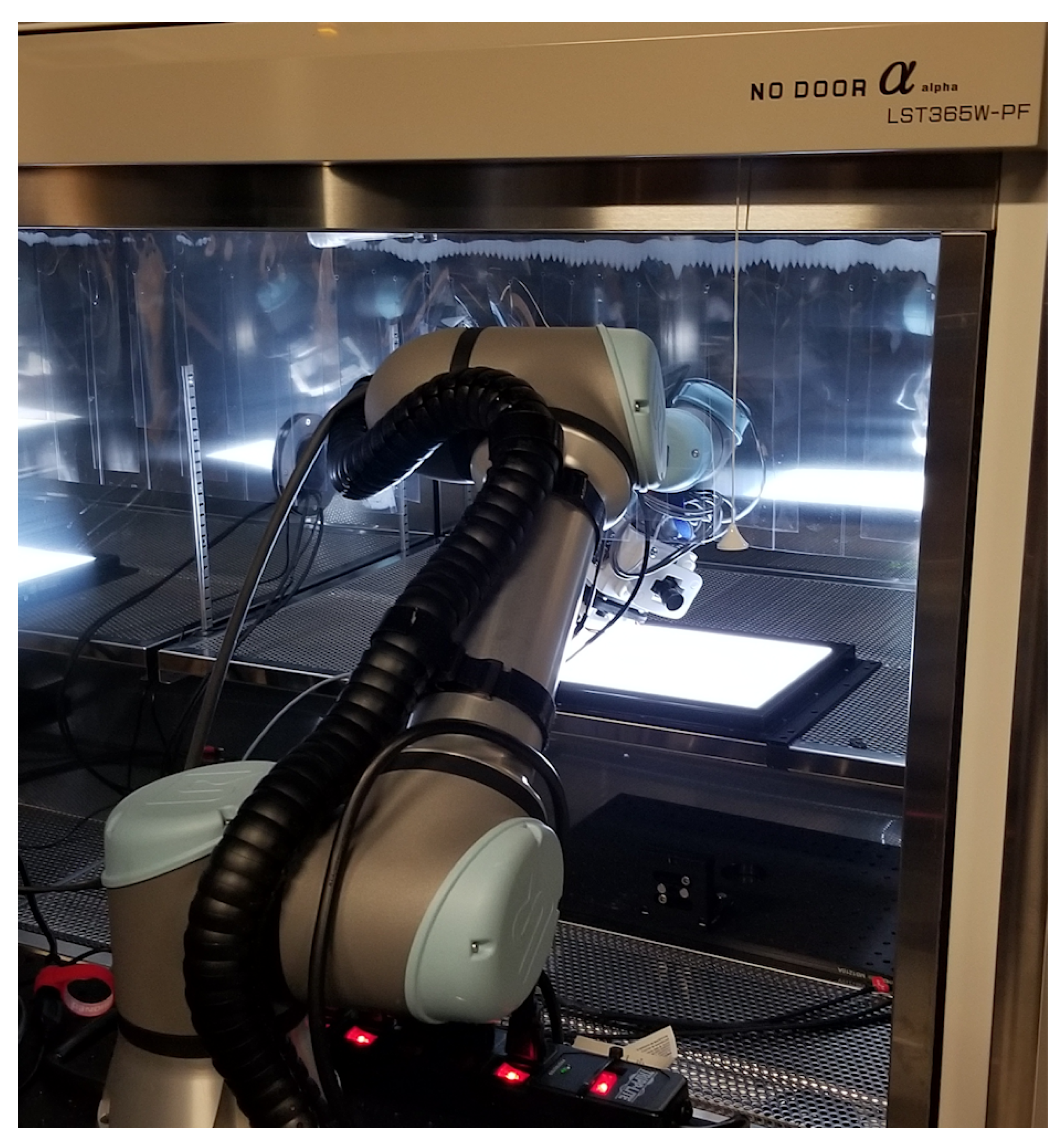
3.2. Instrumentation
4. Related Work
5. Results
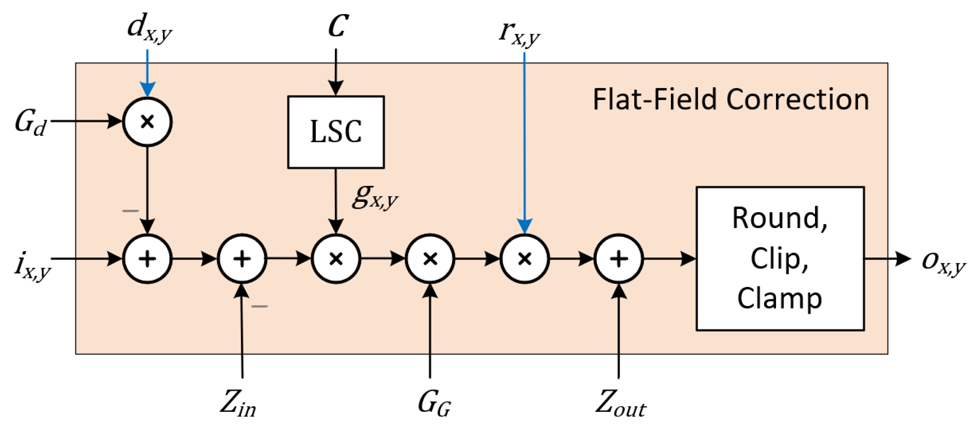
5.1. Flat-Field Correction
5.2. DSNU Analysis
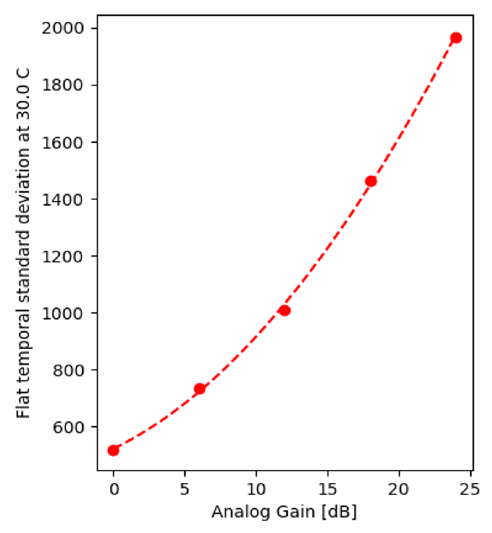
5.2.1. DSNU and Exposure Time
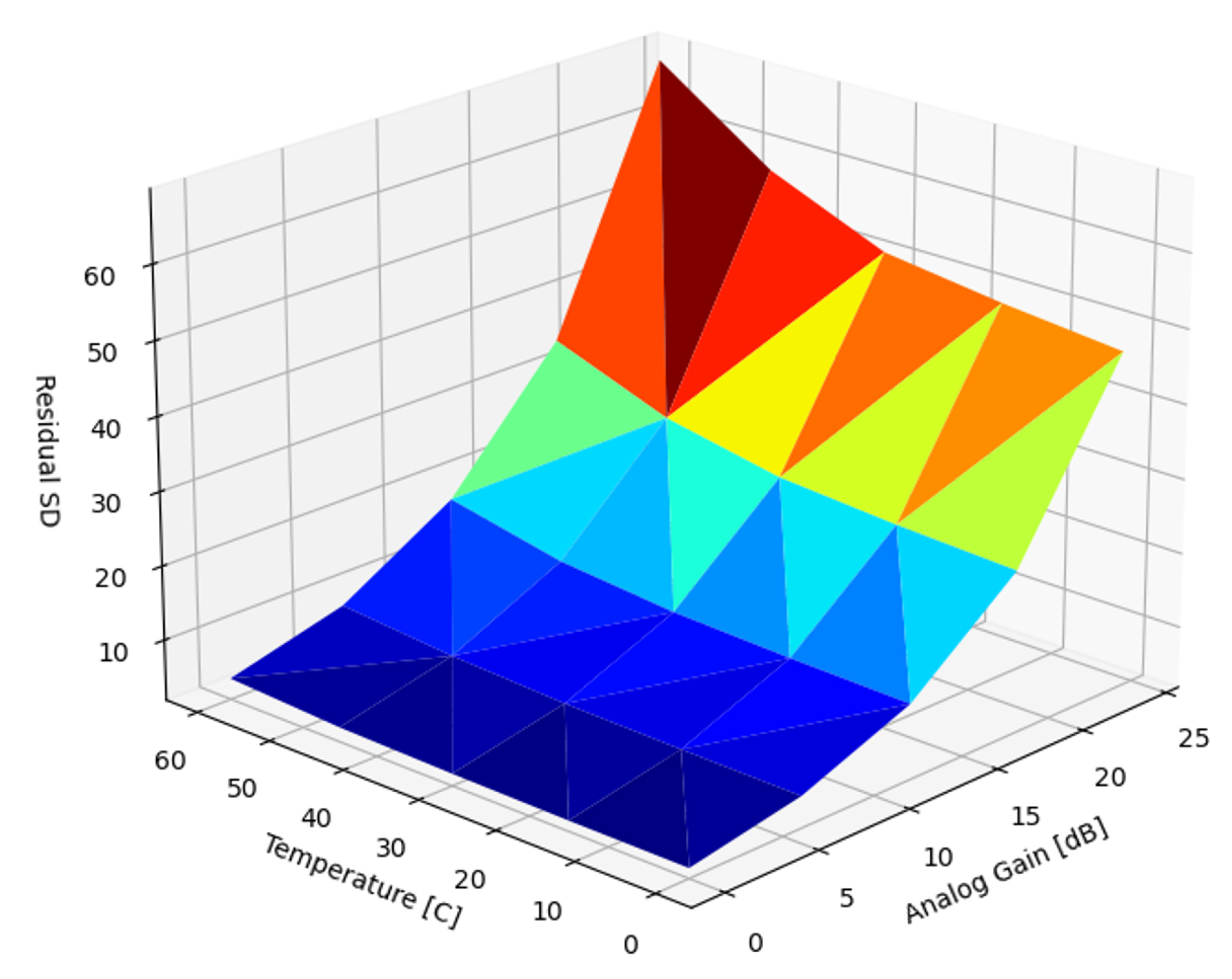
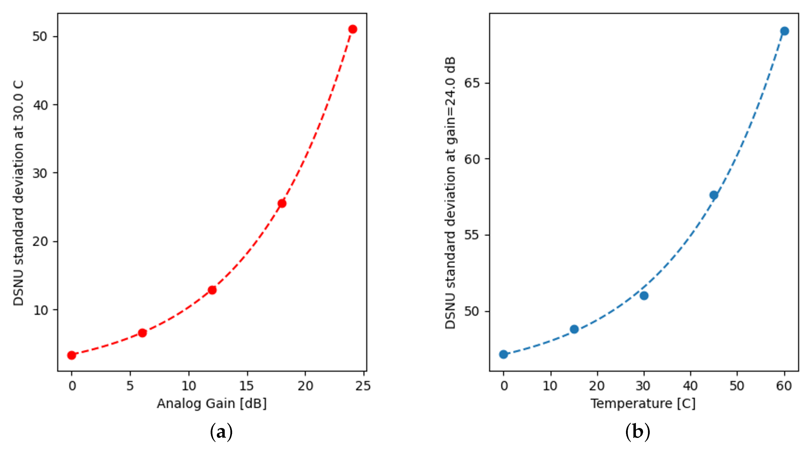
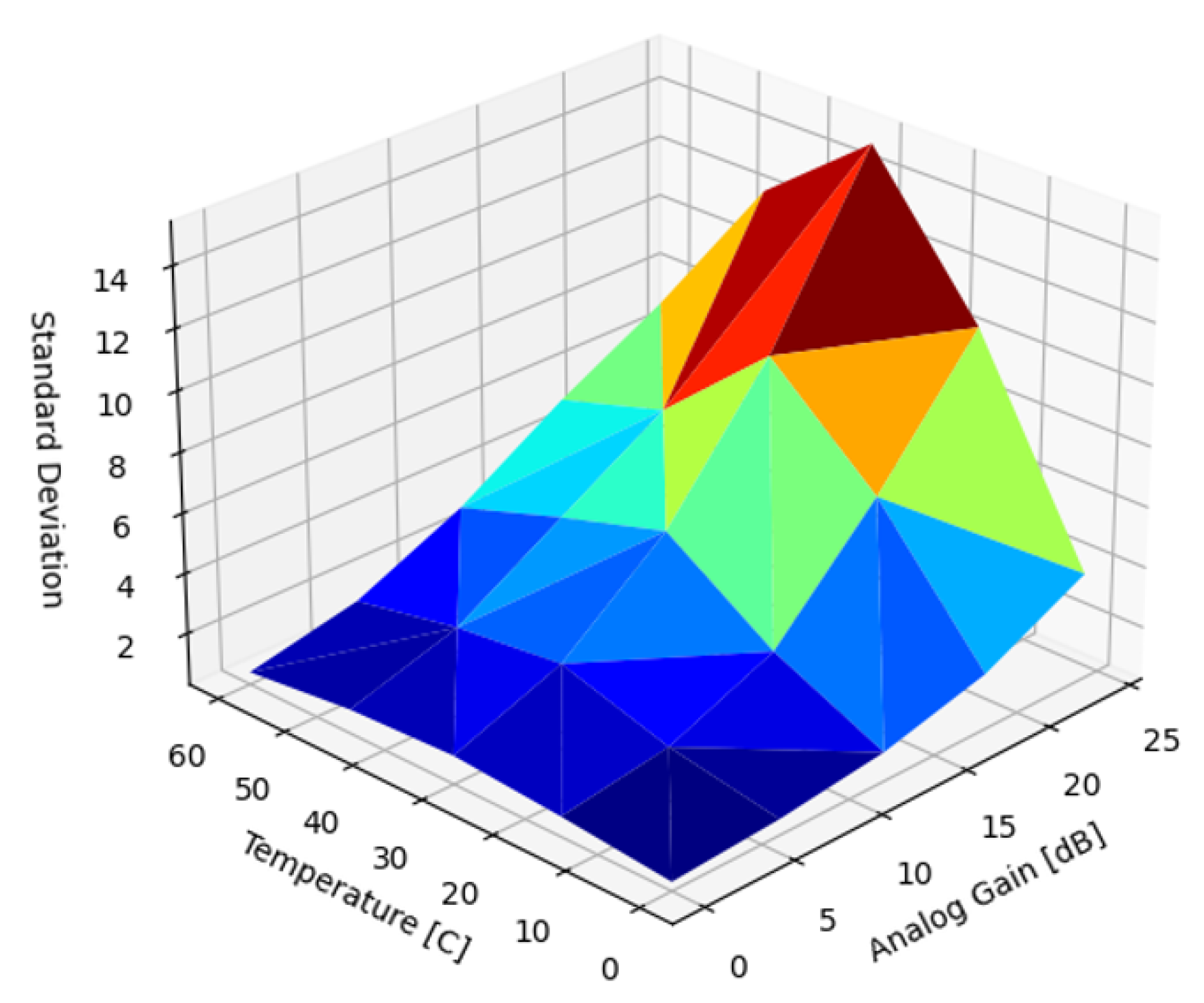
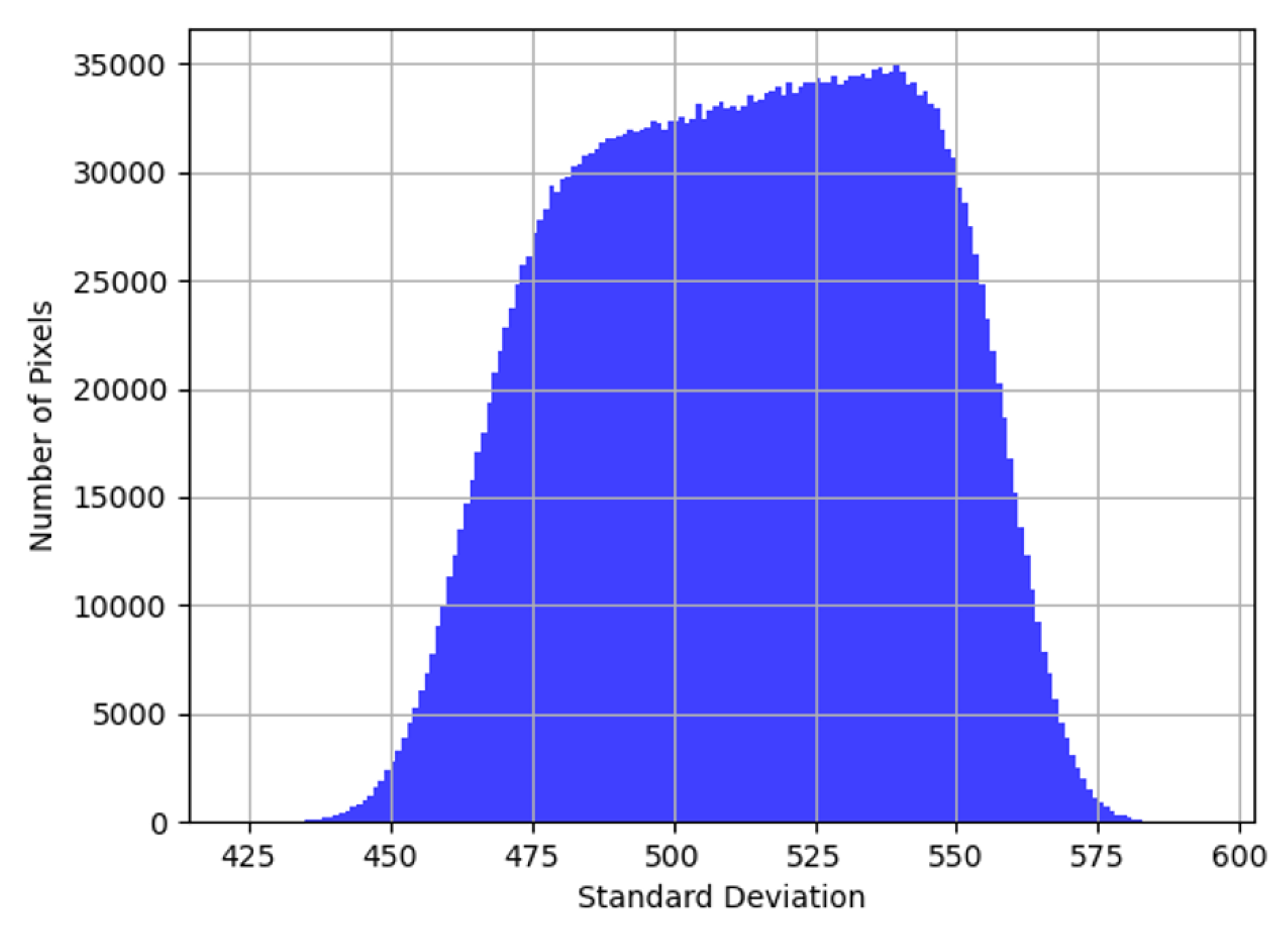
5.2.2. Standard Deviation of Uncorrected DSNU
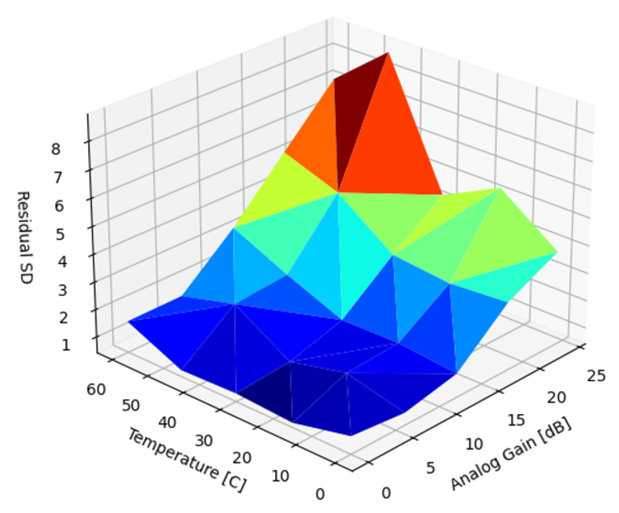
5.2.3. Single-Point Correction
5.2.4. Multipoint Correction
5.2.5. Linear Interpolation between Multiple Reference Images
5.2.6. Single-Point Correction
5.2.7. Optimizing DSNU Reference Selection
- Let denote the probability that during regular operation, the sensor temperature (T) and analog gain () are within a predefined range and , such thatis essentially the 2D probability density function based on discrete parameter , which is a register setting, and continuous parameter T, derived from camera usage statistics.
- Let denote the weight or relative importance of the user application, e.g., disparity mapping, associated with parameter combination . For high-gain scenarios, an increased temporal noise may reduce the importance of DSNU.
5.2.8. Correction with Logarithmic Interpolation
5.3. PRNU Analysis
5.3.1. PRNU and Exposure Time
5.3.2. PRNU and Exposure Time
5.3.3. Analysis of Flat-Field Image Stacks
5.3.4. Standard Deviation of Uncorrected PRNU
5.3.5. Single-Point Correction
5.3.6. Multipoint Correction
6. Discussion
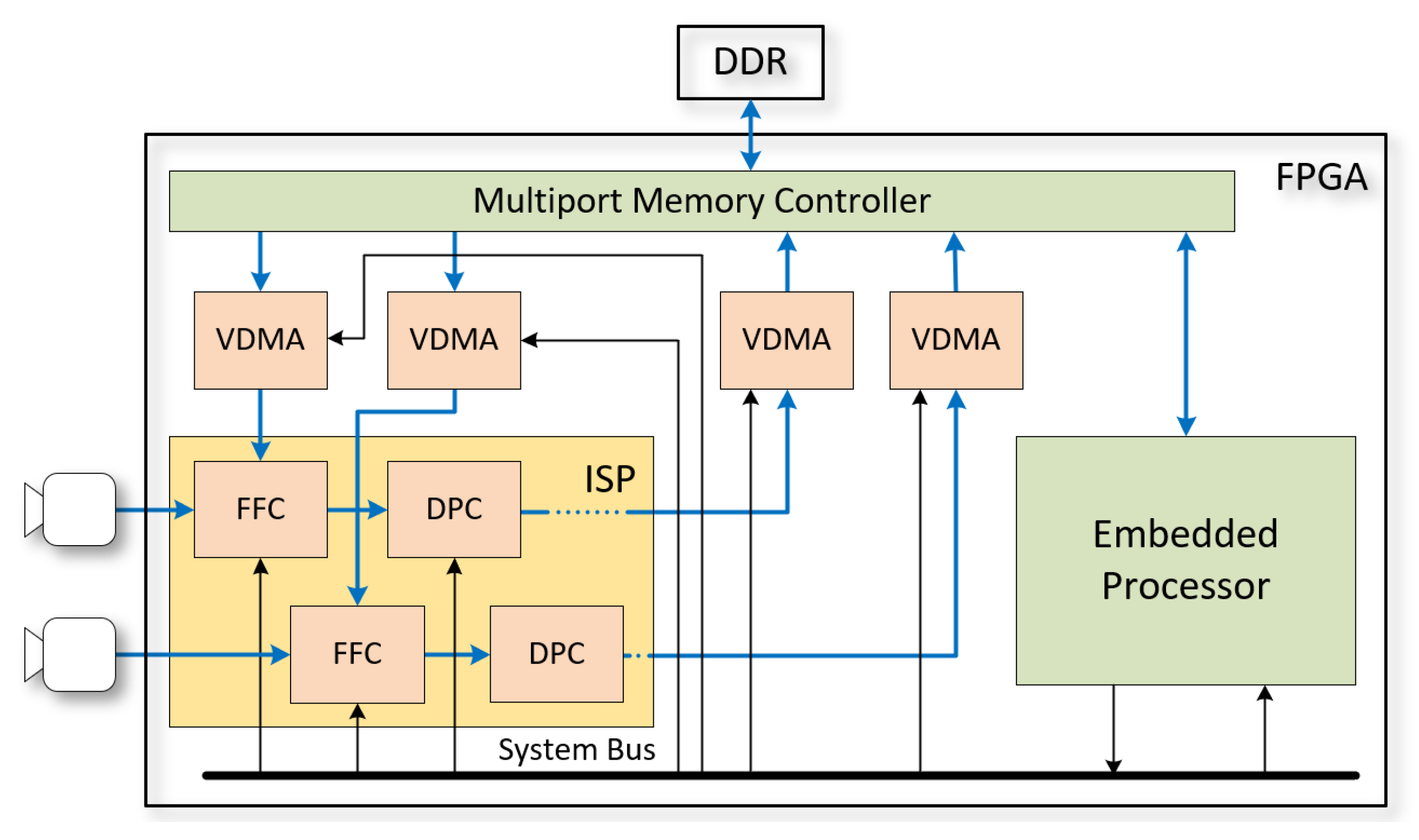
- The most egregious nonuniformity problem is uncorrected lens shading. For consumer products with inexpensive CMOS sensors and optics, such as webcams, a minimal ISP solution can use population images, captured once per manufactured batch, for lens shading correction, and no correction for DSNU or PRNU. Objectionable to human observers, and detrimental to machine vision and processing algorithms, lens shading can be compensated using just the parametric LSC module in the proposed FFC solution. This performance tier does not require an external frame buffer, VDMAs, or FW initialization of the correction buffers ( and ).
- For video applications where visible FPN is not acceptable, such as cell phones and DSLR cameras, the PRNU and DSNU has to be suppressed. This performance tier requires an external frame buffer, and VDMAs around the ISP block to provide and . If fixed -focus optics are used, and the temperature compensation of the lens is not a requirement, LSC can be performed by convolving the intensity correction with PRNU correction in . The results of Section 5.2.3 demonstrated that using a single, static image did not correct the DSNU sufficiently. As temperature and sensor gain change, this method may introduce more noise than originally present in the sensor image.
- The top performance tier is suitable for high-end machine vision cameras, studio equipment, or computational photography where motion-compensated image stacks are registered to suppress temporal noise. For these demanding applications gain- and temperature-compensated DSNU, PRNU, and LSC are all utilized. Parametric LSC is suggested with module-specific, temperature-compensated lens shading parameters accounting for zoom and focus settings. For this tier, FW needs to either calculate or gather image statistics from the OBP region of the sensor and calculate (Section 5.2). Moreover, FW may dynamically adjust the frame buffer contents to interpolate between DSNU and PRNU frames stored in DDR memory. As demonstrated in Section 5.2.3, DSNU correction can be significantly improved by using the global DNSU amplifier () feature of the FFC. PRNU suppression can be improved by using gain-dependent calibration images (). For this performance tier, at initialization, multiple images need to be deposited into DDR memory by FW. During use, FW also needs to read out sensor temperature T, and based on the current analog gain setting , update and reprogram the VDMA read controller to point to the best matched to operating conditions.
7. Future Work
8. Summary
Author Contributions
Funding
Institutional Review Board Statement
Informed Consent Statement
Data Availability Statement
Acknowledgments
Conflicts of Interest
Abbreviations
| ADC | Analog-to-digital converter |
| ASIC | Application-specific integrated circuit |
| CDS | Correlated double sampling |
| CMOS | Complementary metal–oxide semiconductor |
| CNN | Convolutional neural network |
| DDS | Differential delta sampling |
| DDR | Double data rate random-access memory |
| DSNU | Dark signal nonuniformity |
| FFC | Flat-field correction |
| FPA | Focal plane array |
| FPGA | Field-programmable gate array |
| FPN | Fixed-pattern noise |
| FW | Firmware |
| ISP | Image signal processor |
| IR | Infrared |
| LSC | Lens shading correction |
| LED | Light-emitting diode |
| MPSoC | Multiprocessor system on a chip |
| PGA | Programmable gain amplifier |
| PRNU | Photoresponse nonuniformity |
| RST | Reset |
| SD | Standard deviation |
| SEL | Select |
| SH | Sample and hold |
| SoC | System on a chip |
| TEC | Thermoelectric cooler |
| TX | Transmit |
| VDMA | Video direct memory access |
References
- Mooney, J.M.; Sheppard, F.D.; Ewing, W.S.; Ewing, J.E.; Silverman, J. Responsivity Nonuniformity Limited Performance of Infrared Staring Cameras. Opt. Eng. 1989, 28, 281151. [Google Scholar] [CrossRef]
- Perry, D.L.; Dereniak, E.L. Linear theory of nonuniformity correction in infrared staring sensors. Opt. Eng. 1993, 32, 1854–1859. [Google Scholar] [CrossRef]
- Schulz, M.; Caldwell, L. Nonuniformity correction and correctability of infrared focal plane arrays. Infrared Phys. Technol. 1995, 36, 763–777. [Google Scholar] [CrossRef]
- Nakamura, J. Dark Current. In Image Sensors and Signal Processing for Digital Still Cameras, 1st ed.; Taylor and Francis: Boca Ranton, FL, USA, 2006; Chapter Basics of Image Sensors; pp. 68–71. ISBN 0849335450. [Google Scholar]
- Seo, M.W.; Yasutomi, K.; Kagawa, K.; Kawahito, S. A Low Noise CMOS Image Sensor with Pixel Optimization and Noise Robust Column-parallel Readout Circuits for Low-light Levels. ITE Trans. Media Technol. Appl. 2015, 3, 258–262. [Google Scholar] [CrossRef]
- Kim, M.K.; Hong, S.K.; Kwon, O.K. A Fast Multiple Sampling Method for Low-Noise CMOS Image Sensors with Column-Parallel 12-bit SAR ADCs. Sensors 2016, 16, 27. [Google Scholar] [CrossRef] [PubMed]
- Takayanagi, I. Fixed Pattern Noise Suppression. In Image Sensors and Signal Processing for Digital Still Cameras, 1st ed.; Taylor and Francis: Boca Ranton, FL, USA, 2006; Chapter CMOS Image Sensors; pp. 147–161. ISBN 0849335450. [Google Scholar]
- Mei, L.; Zhang, L.; Kong, Z.; Li, H. Noise modeling, evaluation and reduction for the atmospheric lidar technique employing an image sensor. Opt. Commun. 2018, 426, 463–470. [Google Scholar] [CrossRef]
- Teledyne. EV76C661 1.3 Mpixel CMOS Image Sensor. 2019. Available online: https://imaging.teledyne-e2v.com/content/uploads/2019/02/DSC_EV76C661.pdf (accessed on 29 October 2022).
- EMVA. European Machine Vision Association (EMVA) Standard 1288, Standard for Characterization of Image Sensors and Cameras. 2016. Available online: https://www.emva.org/wp-content/uploads/EMVA1288-3.1a.pdf (accessed on 29 October 2022).
- Scharstein, D.; Szeliski, R. High-accuracy stereo depth maps using structured light. In Proceedings of the 2003 IEEE Computer Society Conference on Computer Vision and Pattern Recognition, Madison, WI, USA, 18–20 June 2003; Volume 1, pp. 195–202. [Google Scholar] [CrossRef]
- Liu, L.; Zhang, T. Optics Temperature-Dependent Nonuniformity Correction Via ℓ0-Regularized Prior for Airborne Infrared Imaging Systems. IEEE Photonics J. 2016, 8, 1–10. [Google Scholar] [CrossRef]
- Guan, J.; Lai, R.; Xiong, A.; Liu, Z.; Gu, L. Fixed pattern noise reduction for infrared images based on cascade residual attention CNN. Neurocomputing 2020, 377, 301–313. [Google Scholar] [CrossRef]
- Karaküçük, A.; Dirik, A.E. Adaptive photo-response non-uniformity noise removal against image source attribution. Digit. Investig. 2015, 12, 66–76. [Google Scholar] [CrossRef]
- Burggraaff, O.; Schmidt, N.; Zamorano, J.; Pauly, K.; Pascual, S.; Tapia, C.; Spyrakos, E.; Snik, F. Standardized spectral and radiometric calibration of consumer cameras. Opt. Express 2019, 27, 19075–19101. [Google Scholar] [CrossRef] [PubMed]
- Wang, Y.; Wan, B.; Fu, G.; Su, Y. PRNU Estimation of Linear CMOS Image Sensors That Allows Nonuniform Illumination. IEEE Trans. Instrum. Meas. 2021, 70, 1–11. [Google Scholar] [CrossRef]
- CAL3. Image Engineering “CAL3 V2 Data Sheet”. 2016. Available online: http://www.image-engineering.de/content/products/equipment/illumination_devices/cal3/downloads/CAL3_data_sheet.pdf (accessed on 29 October 2022).
- Seibert, J.A.; Boone, J.M.; Lindfors, K.K. (Eds.) Flat-field correction technique for digital detectors. In Proceedings of Medical Imaging 1998: Physics of Medical Imaging; Society of Photographic Instrumentation Engineers (SPIE): San Diego, CA, USA, 1998; Volume 3336, pp. 348–354. [Google Scholar] [CrossRef]
- Snyder, D.L.; Angelisanti, D.L.; Smith, W.H.; Dai, G.M. Correction for nonuniform flat-field response in focal plane arrays. In Proceedings of SPIE 2827, Digital Image Recovery and Synthesis III; Idell, P.S., Schulz, T.J., Eds.; Society of Photographic Instrumentation Engineers (SPIE): Denver, CO, USA, 1996; Volume 2827, pp. 60–67. [Google Scholar] [CrossRef]
- Ratliff, B.M.; Hayat, M.M.; Tyo, J.S. Radiometrically accurate scene-based nonuniformity correction for array sensors. J. Opt. Soc. Am. A 2003, 20, 1890–1899. [Google Scholar] [CrossRef] [PubMed]
- Vasiliev, V.; Inochkin, F.; Kruglov, S.; Bronshtein, I. Real-time image processing inside a miniature camera using small-package FPGA. In Proceedings of the International Symposium on Consumer Technologies, St. Petersburg, Russia, 11–12 May 2018; pp. 5–8. [Google Scholar] [CrossRef]
- Bowman, R.W.; Vodenicharski, B.; Collins, J.T.; Stirling, J. Flat-Field and Colour Correction for the Raspberry Pi Camera Module. J. Open Hardw. 2020, 4, 1–9. [Google Scholar] [CrossRef]
- Zhang, Z.; Wang, Y.; Piestun, R.; Huang, Z.-L. Characterizing and correcting camera noise in back-illuminated sCMOS cameras. Opt. Express 2021, 29, 6668–6690. [Google Scholar] [CrossRef] [PubMed]
- Teledyne-FLIR. 160 × 120 High-Resolution Micro Thermal Camera: Lepton 3 & 3.5. 2022. Available online: https://flir.netx.net/file/asset/15529/original/attachment (accessed on 29 October 2022).
- Silicon and Devices. Hercules 1280 × 1024, 15 µm Pitch, Digital InSb MWIR. 2016. Available online: https://www.scd.co.il/wp-content/uploads/2019/04/HERCULES_brochure_v3_PRINT.pdf (accessed on 29 October 2022).
- Orżanowski, T. Nonuniformity correction algorithm with efficient pixel offset estimation for infrared focal plane arrays. SpringerPlus 2016, 5, 1831. [Google Scholar] [CrossRef]
- Yao, P.; Tu, B.; Xu, S.; Yu, X.; Xu, Z.; Luo, D.; Hong, J. Non-uniformity calibration method of space-borne area CCD for directional polarimetric camera. Opt. Express 2021, 29, 3309–3326. [Google Scholar] [CrossRef] [PubMed]
- Hu, C.; Bai, Y.; Tang, P. Denoising Algorithm for the Pixel-Response Non-uniformity Correction of a Scientific CMOS Under Low Light Conditions. Int. Arch. Photogramm. Remote Sens. Spat. Inf. Sci. 2016, XLI-B3, 749–753. [Google Scholar] [CrossRef]
- Zhu, Y.; Niu, Y.; Lu, W.; Huang, Z.; Zhang, Y.; Chen, Z. A 160 × 120 ROIC with Non-uniformity Calibration for Silicon Diode Uncooled IRFPA. In Proceedings of the 2019 IEEE International Conference on Electron Devices and Solid-State Circuits (EDSSC), Xi’an, China, 12–14 June 2019; pp. 1–3. [Google Scholar] [CrossRef]
- Kirkpatrick, S.; Gelatt, C.D.; Vecchi, M.P. Optimization by Simulated Annealing. Science 1983, 220, 671–680. [Google Scholar] [CrossRef] [PubMed]


| Sensor Type | Temperature (°C) | Analog Gain (dB) | Std. Dev. ms | Std. Dev. ms | Pearson Correlation |
|---|---|---|---|---|---|
| IMX265 | 10 | 2.0 | 1.423 | 1.416 | 0.974 |
| IMX265 | 10 | 24.0 | 26.164 | 26.047 | 0.997 |
| IMX265 | 50 | 2.0 | 3.275 | 4.982 | 0.983 |
| IMX265 | 50 | 24.0 | 60.294 | 60.428 | 0.997 |
| IMX273 | 10 | 2.0 | 4.430 | 4.416 | 0.988 |
| IMX273 | 10 | 24.0 | 52.864 | 52.880 | 0.995 |
| IMX273 | 50 | 2.0 | 4.799 | 5.376 | 0.962 |
| IMX273 | 50 | 24.0 | 64.950 | 65.802 | 0.982 |
| Temperature (°C) | Analog Gain (dB) | (ms) | Original Std. Dev. | Residual Std. Dev. | Pearson Correlation |
|---|---|---|---|---|---|
| 0 | 0 | 0.53 | 3.16 | 26.44 | 0.726 |
| 0 | 24 | 0.02 | 47.17 | 31.43 | 0.761 |
| 15 | 0 | 0.51 | 3.23 | 25.99 | 0.840 |
| 15 | 24 | 0.02 | 48.82 | 27.94 | 0.867 |
| 30 | 0 | 0.49 | 3.43 | 25.49 | 0.929 |
| 30 | 24 | 0.01 | 50.99 | 26.01 | 0.939 |
| 45 | 0 | 0.46 | 3.76 | 24.98 | 0.977 |
| 45 | 6 | 0.23 | 7.34 | 21.39 | 0.991 |
| 45 | 12 | 0.10 | 14.44 | 14.36 | 0.995 |
| 45 | 18 | 0.05 | 28.64 | 2.80 | 0.995 |
| 45 | 24 | 0.01 | 57.63 | 29.28 | 0.995 |
| 60 | 0 | 0.45 | 4.64 | 24.44 | 0.920 |
| 60 | 6 | 0.21 | 8.69 | 20.75 | 0.948 |
| 60 | 12 | 0.10 | 17.71 | 13.62 | 0.939 |
| 60 | 18 | 0.04 | 34.43 | 12.23 | 0.941 |
| 60 | 24 | 0.01 | 68.42 | 42.62 | 0.940 |
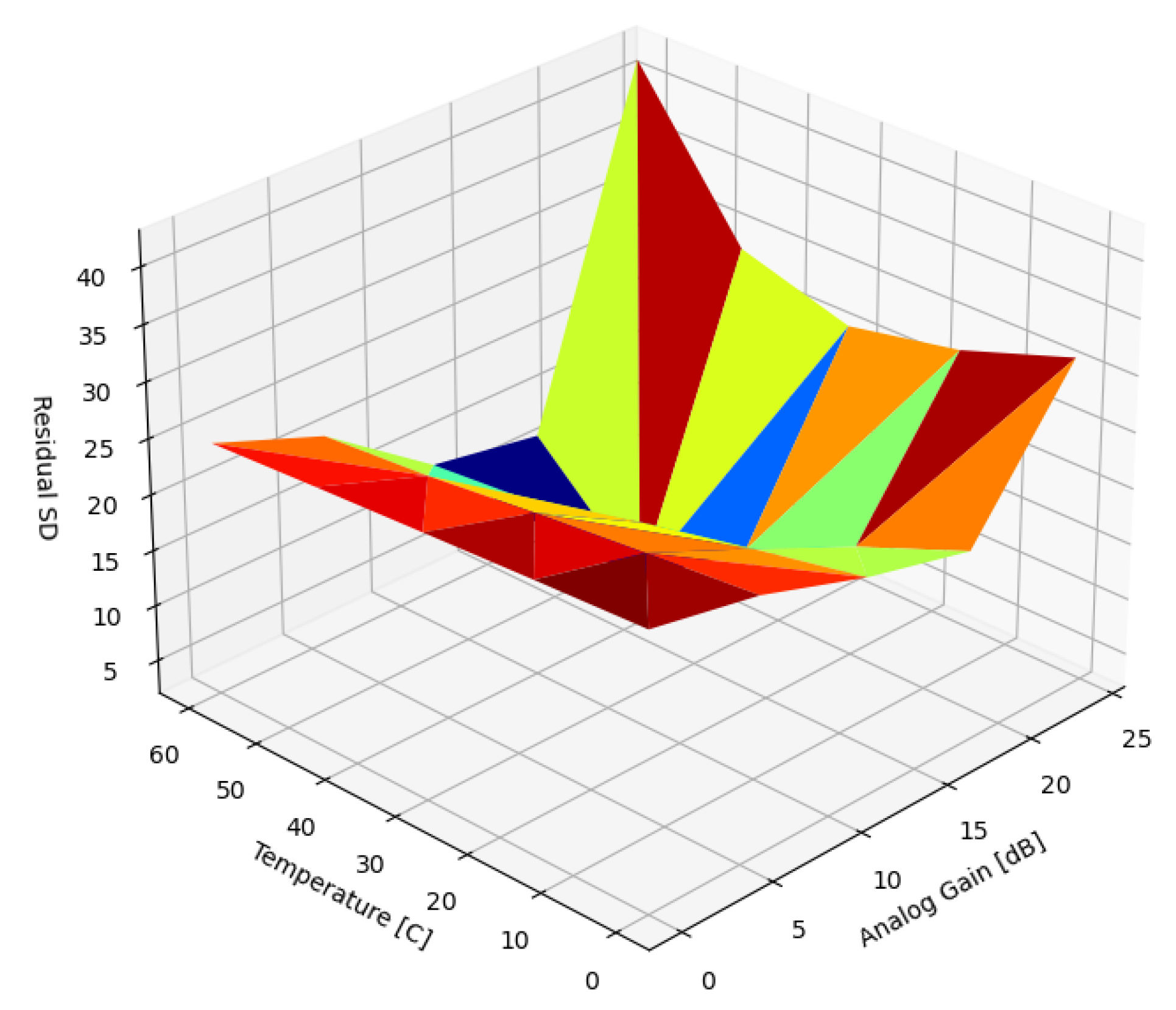
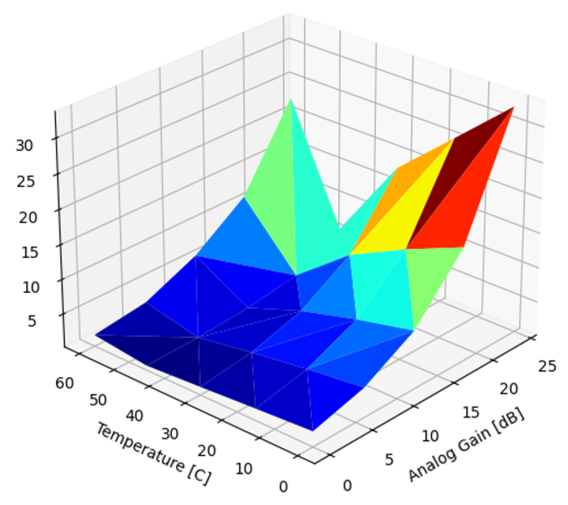
| Temperature (°C) | Analog Gain (dB) | Frame SD | Residual SD | Pearson Correlation | DSNU Reduction (%) | DSNU Reduction (dB) |
|---|---|---|---|---|---|---|
| 0 | 12 | 11.90 | 1.28 | 0.994 | 89.3 | 19.39 |
| 0 | 24 | 47.17 | 3.82 | 0.997 | 91.9 | 21.84 |
| 0 | 18 | 23.61 | 2.89 | 0.993 | 87.8 | 18.24 |
| 0 | 6 | 6.05 | 0.87 | 0.990 | 85.7 | 16.88 |
| 0 | 0 | 3.16 | 1.06 | 0.944 | 66.6 | 9.52 |
| 15 | 24 | 48.82 | 5.33 | 0.994 | 89.1 | 19.24 |
| 15 | 18 | 24.40 | 2.73 | 0.994 | 88.8 | 19.01 |
| ⋮ | ⋮ | ⋮ | ⋮ | ⋮ | ⋮ | ⋮ |
| 45 | 12 | 14.44 | 2.28 | 0.987 | 84.2 | 16.02 |
| 45 | 6 | 7.34 | 2.12 | 0.958 | 71.1 | 10.80 |
| 45 | 0 | 3.76 | 0.65 | 0.985 | 82.8 | 15.30 |
| 60 | 24 | 68.42 | 7.10 | 0.995 | 89.6 | 19.69 |
| 60 | 18 | 34.43 | 5.17 | 0.989 | 85.0 | 16.47 |
| 60 | 12 | 17.71 | 3.21 | 0.984 | 81.9 | 14.84 |
| 60 | 6 | 8.69 | 1.56 | 0.984 | 82.0 | 14.90 |
| 60 | 0 | 4.64 | 1.55 | 0.944 | 66.6 | 9.52 |
| Sensor Type | Temperature (°C) | Analog Gain (dB) | Std. Dev. ms | Std. Dev. ms | Pearson Correlation |
|---|---|---|---|---|---|
| IMX265 | 0 | 2.0 | 175.69 | 176.00 | 0.999141 |
| IMX265 | 20 | 2.0 | 174.47 | 176.33 | 0.999050 |
| IMX265 | 60 | 2.0 | 171.03 | 174.16 | 0.998582 |
| IMX273 | 35 | 0.2 | 182.69 | 183.31 | 0.996231 |
| IMX273 | 35 | 12.0 | 180.74 | 183.32 | 0.995280 |
| IMX273 | 60 | 0.2 | 177.80 | 181.75 | 0.999082 |
| IMX273 | 60 | 12.0 | 154.77 | 155.31 | 0.996216 |
Publisher’s Note: MDPI stays neutral with regard to jurisdictional claims in published maps and institutional affiliations. |
© 2022 by the authors. Licensee MDPI, Basel, Switzerland. This article is an open access article distributed under the terms and conditions of the Creative Commons Attribution (CC BY) license (https://creativecommons.org/licenses/by/4.0/).
Share and Cite
Becker, G.S.; Lovas, R. Uniformity Correction of CMOS Image Sensor Modules for Machine Vision Cameras. Sensors 2022, 22, 9733. https://doi.org/10.3390/s22249733
Becker GS, Lovas R. Uniformity Correction of CMOS Image Sensor Modules for Machine Vision Cameras. Sensors. 2022; 22(24):9733. https://doi.org/10.3390/s22249733
Chicago/Turabian StyleBecker, Gabor Szedo, and Róbert Lovas. 2022. "Uniformity Correction of CMOS Image Sensor Modules for Machine Vision Cameras" Sensors 22, no. 24: 9733. https://doi.org/10.3390/s22249733
APA StyleBecker, G. S., & Lovas, R. (2022). Uniformity Correction of CMOS Image Sensor Modules for Machine Vision Cameras. Sensors, 22(24), 9733. https://doi.org/10.3390/s22249733